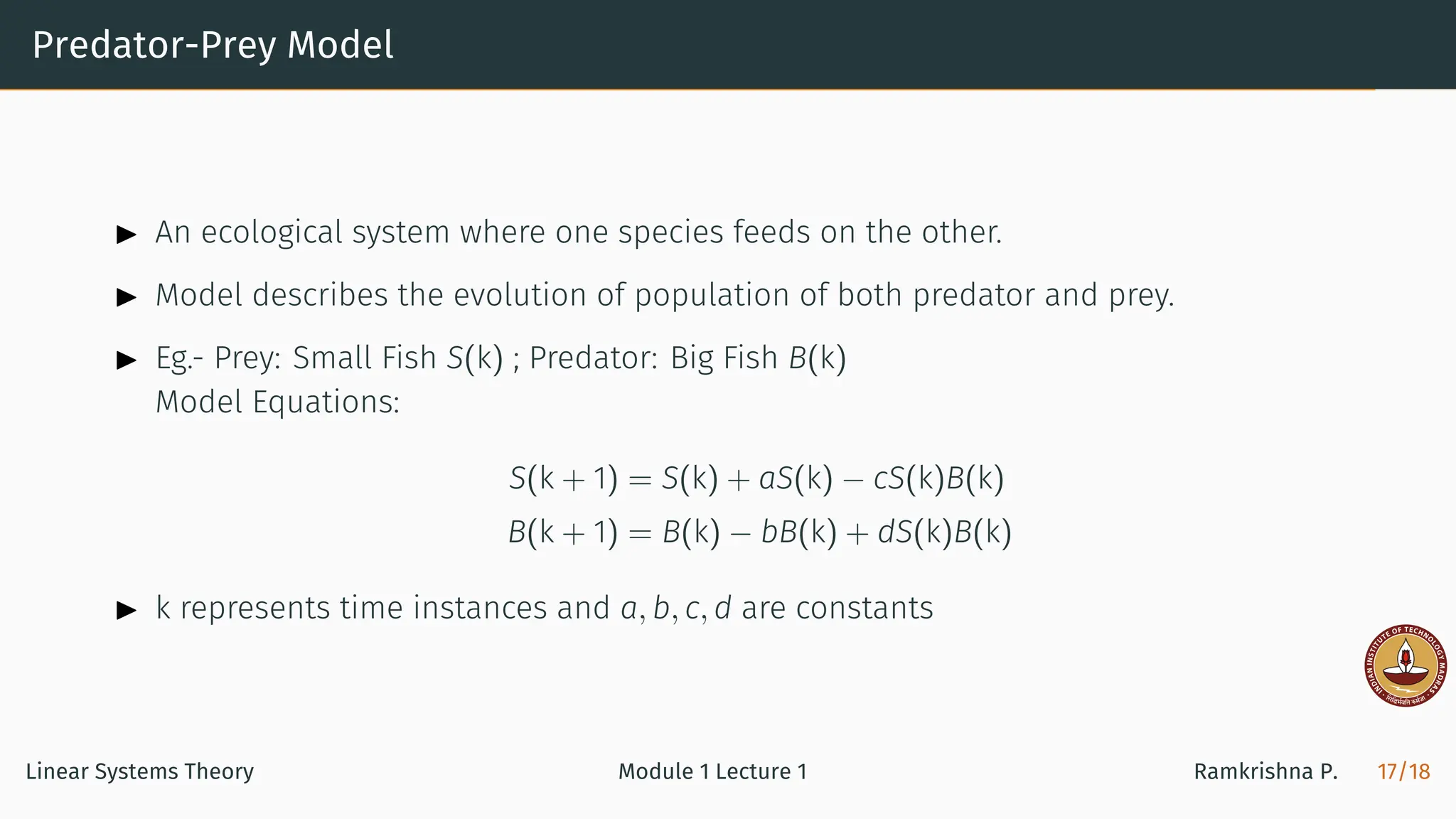
This document provides an introduction to linear systems theory, emphasizing the significance of mathematical models to represent and predict the behavior of dynamic systems. It discusses the key components of modeling, including inductance, mass, and the mass-spring-damper system, offering examples of both mechanical and electrical systems. The document also covers ecological modeling through a predator-prey model, showcasing the oscillatory nature of population dynamics.

1. Linear Systems Theory
Ramkrishna Pasumarthy
Department of Electrical Engineering,
Indian Institute of Technology Madras

2. Module 1
Lecture 1
Introduction to Linear Systems
Linear Systems Theory Module 1 Lecture 1 Ramkrishna P. 1/18

3. Engineering Tools
Linear Systems Theory Module 1 Lecture 1 Ramkrishna P. 2/18

4. The Importance of Math
On Teaching Mathematics https://www.uni-muenster.de/Physik.TP/ munsteg/arnold.html
▶ Mathematics is a part of physics.
Linear Systems Theory Module 1 Lecture 1 Ramkrishna P. 3/18

5. The Importance of Math
On Teaching Mathematics https://www.uni-muenster.de/Physik.TP/ munsteg/arnold.html
▶ Mathematics is a part of physics.
▶ Physics is an experimental science, a part of natural science.
Linear Systems Theory Module 1 Lecture 1 Ramkrishna P. 3/18

6. The Importance of Math
On Teaching Mathematics https://www.uni-muenster.de/Physik.TP/ munsteg/arnold.html
▶ Mathematics is a part of physics.
▶ Physics is an experimental science, a part of natural science.
▶ Mathematics is the part of physics where experiments are cheap.
Linear Systems Theory Module 1 Lecture 1 Ramkrishna P. 3/18

7. System Modelling

8. What is a Model?
▶ Models are mathematical representations to help understand dynamical behaviour
of systems.
▶ Can describe behaviour of a physical process. Eg. How long would it take for a fan to
come to a halt, once switched off?
▶ Can predict response of a system to certain inputs. Eg.- Effect of GST on economy.
▶ This is important because in most cases the system response is not instantaneous,
but evolves with time.
Linear Systems Theory Module 1 Lecture 1 Ramkrishna P. 4/18

9. What is a Good Model?
▶ Depends on the purpose of the model.
▶ Should incorporate the factors that govern the dynamics or evolution of a system
with time.
▶ The same system can be represented by different models.
Eg.- A lumped and distributed parameter model of a transmission line.
▶ The model abstraction must be compact, as opposed to a rule based formulation.
▶ How accurate should the model be?
Linear Systems Theory Module 1 Lecture 1 Ramkrishna P. 5/18

10. Some Basic Modelling Elements
1. Inductance: stores energy in a magnetic field when electric current flows through it.
ϕ ∝ i, v = ϕ̇, v ∝ di
dt
The energy stored in an inductor W =
∫ ϕ
0
i(ϕ)dϕ.
In the linear case W = 1
2
ϕ2
L = 1
2 Li2
2. Mass: An inertia element: Newtons second law
For a point mass M > 0, moving in the x direction, p = Mv in the nonrelativistic case.
From the Newtons second law F = dp
dt .
If the mass is moved by a force, workdone is
Fdx =
dp
dt
dx = vdp =
p
M
dp
Linear Systems Theory Module 1 Lecture 1 Ramkrishna P. 6/18

11. Some Basic Modelling Elements
The Kinetic Energy =
∫ p
0
p
M dp = p2
2M .
Figure 1: Kinetic energy and co-kinetic energy
Linear Systems Theory Module 1 Lecture 1 Ramkrishna P. 7/18

12. Examples of Systems and their
Models

13. A Simple Mechanical System
▶ One of the most simple models is a mass-spring-damper system.
▶ Unforced system - Model equation:
mẍ + dẋ + kx = 0.
▶ m represents the mass, k the spring constant, and d is the damping coefficient.
▶ x ∈ R is a variable which denotes the position of the mass w.r.t its rest position.
▶ ẋ and ẍ respectively denoting the velocity and acceleration respectively.
Linear Systems Theory Module 1 Lecture 1 Ramkrishna P. 8/18

14. A Simple Mechanical System
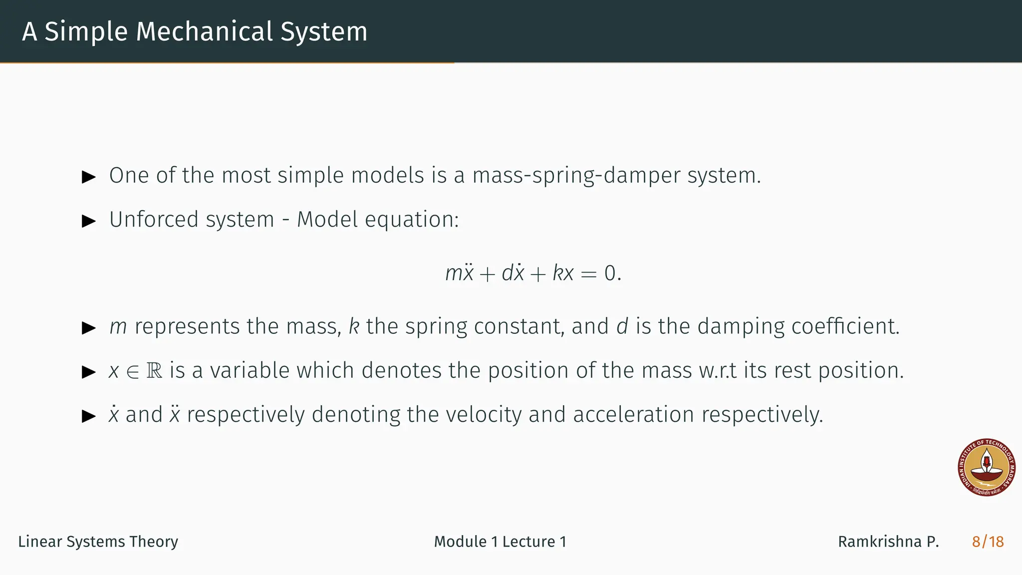
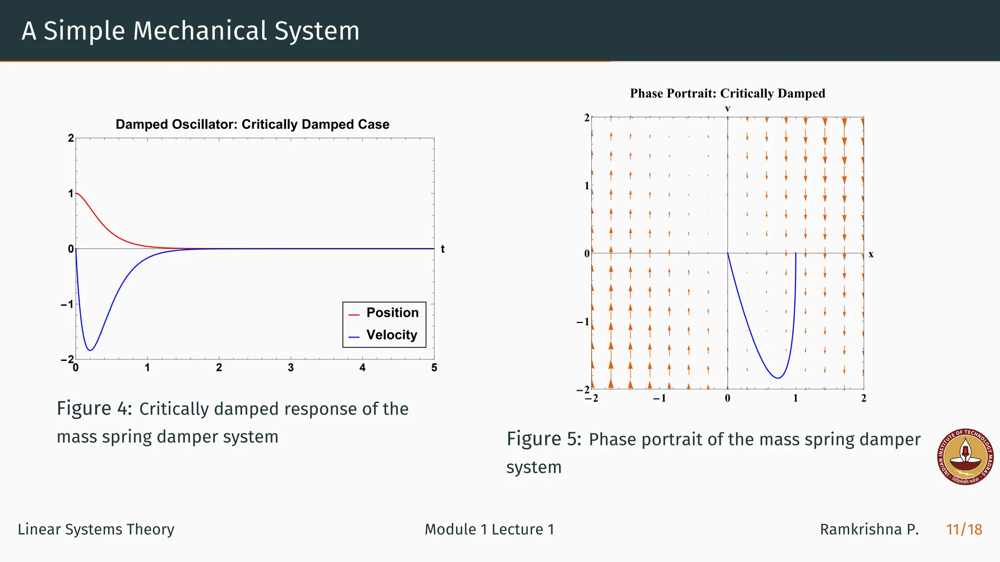
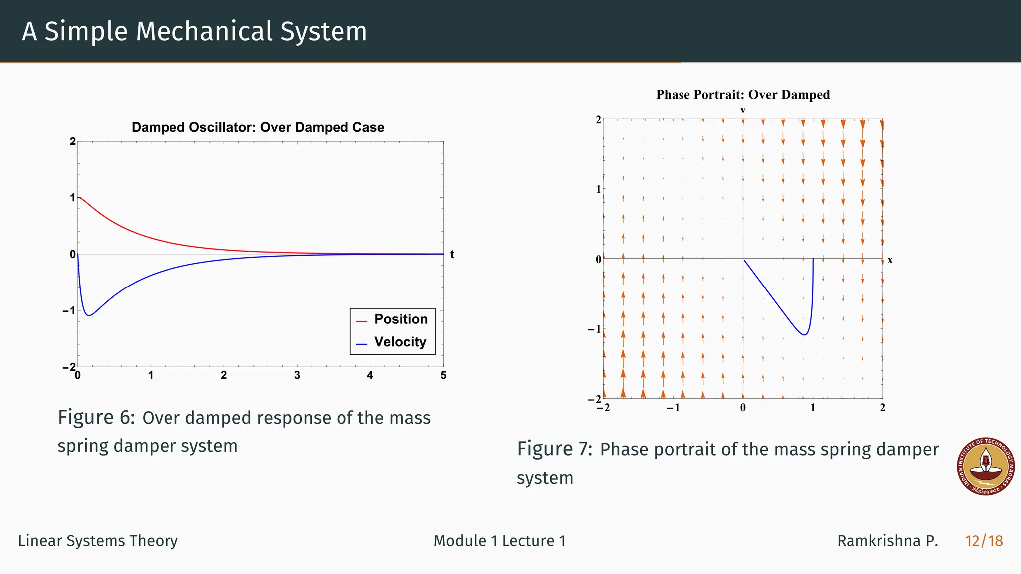
▶ This system can also be written as
x = x1
ẋ1 = x2
ẋ2 = −
d
m
x2 −
k
m
x1
▶ Or in a structured way of the form
[
ẋ1
ẋ2
]
=
[
0 1
− k
m − d
m
]
| {z }
The state matrix A
[
x1
x2
]
|{z}
state vector x
ẋ = Ax
Linear Systems Theory Module 1 Lecture 1 Ramkrishna P. 9/18

15. A Simple Mechanical System
0 2 4 6 8 10 12 14
-4
-2
0
2
4
t
Position
Velocity
Damped Oscillator: Under Damped Case
Figure 2: Under damped response of the mass
spring damper system
-2 -1 0 1 2
-4
-2
0
2
4
x
v
Phase Portrait: Under Damped
Figure 3: Phase portrait of the mass spring damper
system
Linear Systems Theory Module 1 Lecture 1 Ramkrishna P. 10/18

16. A Simple Mechanical System
0 1 2 3 4 5
-2
-1
0
1
2
t
Position
Velocity
Damped Oscillator: Critically Damped Case
Figure 4: Critically damped response of the
mass spring damper system
-2 -1 0 1 2
-2
-1
0
1
2
x
v
Phase Portrait: Critically Damped
Figure 5: Phase portrait of the mass spring damper
system
Linear Systems Theory Module 1 Lecture 1 Ramkrishna P. 11/18

17. A Simple Mechanical System
0 1 2 3 4 5
-2
-1
0
1
2
t
Position
Velocity
Damped Oscillator: Over Damped Case
Figure 6: Over damped response of the mass
spring damper system
-2 -1 0 1 2
-2
-1
0
1
2
x
v
Phase Portrait: Over Damped
Figure 7: Phase portrait of the mass spring damper
system
Linear Systems Theory Module 1 Lecture 1 Ramkrishna P. 12/18

18. A Simple Electrical System
▶ Series RLC Circuit with voltage source
▶ The governing equations of the system are
V = RiL + L
diL
dt
+ vC
iL = C
dvC
dt
▶ Written in the state space form as
[
dvC
dt
diL
dt
]
=
[
0 1
C
−1
L −R
L
]
| {z }
A
[
vC
iL
]
|{z}
x
+
[
0
1
L
]
|{z}
The input matrix B
V (The Control input u)
ẋ = Ax + Bu
Linear Systems Theory Module 1 Lecture 1 Ramkrishna P. 13/18

19. A Simple Electrical System
Impulse Response
0 0.01 0.02 0.03 0.04 0.05 0.06 0.07 0.08 0.09 0.1
Time [s]
-1
0
1
2
3
4
5
Current
[A]
10-5 Current for Impulse Input
Figure 8: Current through the RLC circuit
0 0.01 0.02 0.03 0.04 0.05 0.06 0.07 0.08 0.09 0.1
Time [s]
-0.5
0
0.5
1
1.5
2
2.5
Voltage
[V]
10-3 Voltage across Capacitor for Impulse Input
Figure 9: Voltage across the capacitor
Linear Systems Theory Module 1 Lecture 1 Ramkrishna P. 14/18

20. A Simple Electrical System
Step Response
0 0.01 0.02 0.03 0.04 0.05 0.06 0.07 0.08 0.09 0.1
Time [s]
-0.5
0
0.5
1
1.5
2
2.5
3
3.5
Current
[A]
10-3 Current for Step Input
Figure 10: Current through the RLC circuit
0 0.01 0.02 0.03 0.04 0.05 0.06 0.07 0.08 0.09 0.1
Time [s]
0
0.2
0.4
0.6
0.8
1
1.2
Voltage
[V]
Voltage across Capacitor for Step Input
Figure 11: Voltage across the capacitor
Linear Systems Theory Module 1 Lecture 1 Ramkrishna P. 15/18

21. A Simple Electrical System
Response to Sinusoidal Input
0 0.2 0.4 0.6 0.8 1 1.2 1.4 1.6 1.8 2
Time [s]
-1
-0.8
-0.6
-0.4
-0.2
0
0.2
0.4
0.6
0.8
1
Current
[A]
10-4 Current for Sinusoidal Input
Figure 12: Current through the RLC circuit
0 0.2 0.4 0.6 0.8 1 1.2 1.4 1.6 1.8 2
Time [s]
-1
-0.8
-0.6
-0.4
-0.2
0
0.2
0.4
0.6
0.8
1
Voltage
[V]
Voltage across Capacitor for Sinusoidal Input
Figure 13: Voltage across the capacitor
Linear Systems Theory Module 1 Lecture 1 Ramkrishna P. 16/18

22. Predator-Prey Model
▶ An ecological system where one species feeds on the other.
▶ Model describes the evolution of population of both predator and prey.
▶ Eg.- Prey: Small Fish S(k) ; Predator: Big Fish B(k)
Model Equations:
S(k + 1) = S(k) + aS(k) − cS(k)B(k)
B(k + 1) = B(k) − bB(k) + dS(k)B(k)
▶ k represents time instances and a, b, c, d are constants
Linear Systems Theory Module 1 Lecture 1 Ramkrishna P. 17/18

23. Predator-Prey Model
▶ The populations of both the small and Big fish are oscillatory in nature.
0 10 20 30 40 50 60 70 80 90
Years
0
5
10
15
20
25
30
Population
in
Thousands
Predator Prey Model
Prey
Predator
Figure 14: Population of predator and prey for 90 years
Linear Systems Theory Module 1 Lecture 1 Ramkrishna P. 18/18