Linear Algebra With Applications 8th Edition Leon Solutions Manual Linear Algebra With Applications 8th Edition Leon Solutions Manual Linear Algebra With Applications 8th Edition Leon Solutions Manual

1. Download the full version and explore a variety of test banks
or solution manuals at https://testbankfan.com
Linear Algebra With Applications 8th Edition Leon
Solutions Manual
_____ Tap the link below to start your download _____
https://testbankfan.com/product/linear-algebra-with-
applications-8th-edition-leon-solutions-manual/
Find test banks or solution manuals at testbankfan.com today!

2. We have selected some products that you may be interested in
Click the link to download now or visit testbankfan.com
for more options!.
Linear Algebra with Applications 9th Edition Leon
Solutions Manual
https://testbankfan.com/product/linear-algebra-with-applications-9th-
edition-leon-solutions-manual/
Linear Algebra with Applications 2nd Edition Bretscher
Solutions Manual
https://testbankfan.com/product/linear-algebra-with-applications-2nd-
edition-bretscher-solutions-manual/
Linear Algebra with Applications 5th Edition Bretscher
Solutions Manual
https://testbankfan.com/product/linear-algebra-with-applications-5th-
edition-bretscher-solutions-manual/
Management Information Systems Global 14th Edition Laudon
Test Bank
https://testbankfan.com/product/management-information-systems-
global-14th-edition-laudon-test-bank/

3. Criminal Law and Procedure for the Paralegal 4th Edition
McCord Test Bank
https://testbankfan.com/product/criminal-law-and-procedure-for-the-
paralegal-4th-edition-mccord-test-bank/
Elementary Differential Equations With Boundary Value
Problems 6th Edition Edwards Solutions Manual
https://testbankfan.com/product/elementary-differential-equations-
with-boundary-value-problems-6th-edition-edwards-solutions-manual/
Physical Geography 11th Edition Petersen Solutions Manual
https://testbankfan.com/product/physical-geography-11th-edition-
petersen-solutions-manual/
Life Span Human Development 9th Edition Sigelman Test Bank
https://testbankfan.com/product/life-span-human-development-9th-
edition-sigelman-test-bank/
American Pageant Volume 1 16th Edition Kennedy Test Bank
https://testbankfan.com/product/american-pageant-volume-1-16th-
edition-kennedy-test-bank/

4. Garde Manger Cold Kitchen Fundamentals 1st Edition
Federation Test Bank
https://testbankfan.com/product/garde-manger-cold-kitchen-
fundamentals-1st-edition-federation-test-bank/

5. Another Random Scribd Document
with Unrelated Content

6. Successors of
Cavalieri.
able to effect numerous integrations relating to the areas of portions
of conic sections and the volumes generated by the revolution of
these portions about various axes. At a later date, and partly in
answer to an attack made upon him by Paul Guldin, Cavalieri
published a treatise entitled Exercitationes geometricae sex (1647),
in which he adapted his method to the determination of centres of
gravity, in particular for solids of variable density.
Among the results which he obtained is that which we should
now write
∫x
0 xm dx =
xm+1
, (m integral).
m + 1
He regarded the problem thus solved as that of determining the
sum of the mth powers of all the lines drawn across a
parallelogram parallel to one of its sides.
At this period scientific investigators communicated their results to
one another through one or more intermediate persons. Such
intermediaries were Pierre de Carcavy and Pater Marin Mersenne;
and among the writers thus in communication
were Bonaventura Cavalieri, Christiaan Huygens,
Galileo Galilei, Giles Personnier de Roberval,
Pierre de Fermat, Evangelista Torricelli, and a little
later Blaise Pascal; but the letters of Carcavy or Mersenne would
probably come into the hands of any man who was likely to be
interested in the matters discussed. It often happened that, when
some new method was invented, or some new result obtained, the
method or result was quickly known to a wide circle, although it
might not be printed until after the lapse of a long time. When
Cavalieri was printing his two treatises there was much discussion of

7. Fermat’s
method of
Integration.
the problem of quadratures. Roberval (1634) regarded an area as
made up of “infinitely” many “infinitely” narrow strips, each of which
may be considered to be a rectangle, and he had similar ideas in
regard to lengths and volumes. He knew how to approximate to the
quantity which we express by ∫1
0 xmdx by the process of forming the
sum
0m + 1m + 2m + ... (n − 1)m
,
nm+1
and he claimed to be able to prove that this sum tends to 1/(m + 1),
as n increases for all positive integral values of m. The method of
integrating xm by forming this sum was found also by Fermat (1636),
who stated expressly that he arrived at it by
generalizing a method employed by Archimedes
(for the cases m = 1 and m = 2) in his books on
Conoids and Spheroids and on Spirals (see T. L.
Heath, The Works of Archimedes, Cambridge,
1897). Fermat extended the result to the case where m is fractional
(1644), and to the case where m is negative. This latter extension
and the proofs were given in his memoir, Proportionis geometricae in
quadrandis parabolis et hyperbolis usus, which appears to have
received a final form before 1659, although not published until 1679.
Fermat did not use fractional or negative indices, but he regarded
his problems as the quadratures of parabolas and hyperbolas of
various orders. His method was to divide the interval of integration
into parts by means of intermediate points the abscissae of which
are in geometric progression. In the process of § 5 above, the points
M must be chosen according to this rule. This restrictive condition
being understood, we may say that Fermat’s formulation of the

8. Various
Integrations.
problem of quadratures is the same as our definition of a definite
integral.
The result that the problem of quadratures could be solved for any
curve whose equation could be expressed in the form
y = xm (m ≠ −1),
or in the form
y = a1 xm1 + a2 xm2 + ... + an xmn,
where none of the indices is equal to −1, was used by John Wallis in
his Arithmetica infinitorum (1655) as well as by
Fermat (1659). The case in which m = −1 was
that of the ordinary rectangular hyperbola; and
Gregory of St Vincent in his Opus geometricum
quadraturae circuli et sectionum coni (1647) had proved by the
method of exhaustions that the area contained between the curve,
one asymptote, and two ordinates parallel to the other asymptote,
increases in arithmetic progression as the distance between the
ordinates (the one nearer to the centre being kept fixed) increases in
geometric progression. Fermat described his method of integration
as a logarithmic method, and thus it is clear that the relation
between the quadrature of the hyperbola and logarithms was
understood although it was not expressed analytically. It was not
very long before the relation was used for the calculation of
logarithms by Nicolaus Mercator in his Logarithmotechnia (1668). He
began by writing the equation of the curve in the form y = 1/(1 +
x), expanded this expression in powers of x by the method of
division, and integrated it term by term in accordance with the well-

9. Integration
before the
Integral
Calculus.
Fermat’s
methods of
Differentiation.
understood rule for finding the quadrature of a curve given by such
an equation as that written at the foot of p. 325.
By the middle of the 17th century many mathematicians could
perform integrations. Very many particular results had been
obtained, and applications of them had been
made to the quadrature of the circle and other
conic sections, and to various problems
concerning the lengths of curves, the areas they
enclose, the volumes and superficial areas of
solids, and centres of gravity. A systematic
account of the methods then in use was given, along with much that
was original on his part, by Blaise Pascal in his Lettres de Amos
Dettonville sur quelques-unes de ses inventions en géométrie
(1659).
16. The problem of maxima and minima and the problem of
tangents had also by the same time been effectively solved. Oresme
in the 14th century knew that at a point where the ordinate of a
curve is a maximum or a minimum its variation
from point to point of the curve is slowest; and
Kepler in the Stereometria doliorum remarked
that at the places where the ordinate passes from
a smaller value to the greatest value and then
again to a smaller value, its variation becomes insensible. Fermat in
1629 was in possession of a method which he then communicated to
one Despagnet of Bordeaux, and which he referred to in a letter to
Roberval of 1636. He communicated it to René Descartes early in
1638 on receiving a copy of Descartes’s Géométrie (1637), and with
it he sent to Descartes an account of his methods for solving the
problem of tangents and for determining centres of gravity.

10. Fig. 6.
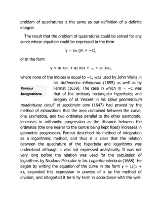
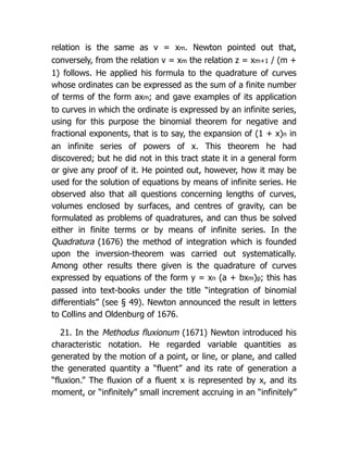
Fermat’s method for maxima and
minima is essentially our method.
Expressed in a more modern notation,
what he did was to begin by connecting
the ordinate y and the abscissa x of a
point of a curve by an equation which
holds at all points of the curve, then to
subtract the value of y in terms of x from the value obtained by
substituting x + E for x, then to divide the difference by E, to
put E = 0 in the quotient, and to equate the quotient to zero.
Thus he differentiated with respect to x and equated the
differential coefficient to zero.
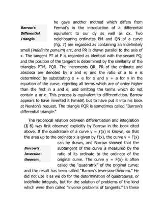
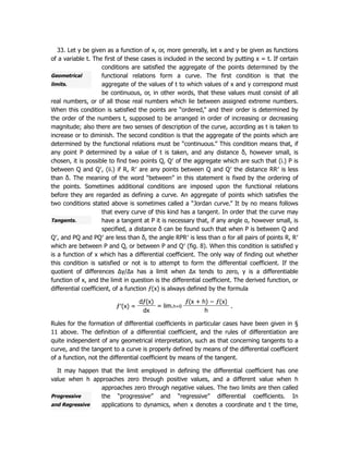
Fermat’s method for solving the problem of tangents may be
explained as follows:—Let (x, y) be the coordinates of a point P
of a curve, (x′, y′), those of a neighbouring point P′ on the
tangent at P, and let MM′ = E (fig. 6).
From the similarity of the triangles P′TM′, PTM we have
y′ : A − E = y : A,
where A denotes the subtangent TM. The point P′ being near
the curve, we may substitute in the equation of the curve x − E
for x and (yA − yE)/A for y. The equation of the curve is
approximately satisfied. If it is taken to be satisfied exactly, the
result is an equation of the form φ(x, y, A, E) = 0, the left-hand
member of which is divisible by E. Omitting the factor E, and
putting E = 0 in the remaining factor, we have an equation
which gives A. In this problem of tangents also Fermat found the
required result by a process equivalent to differentiation.

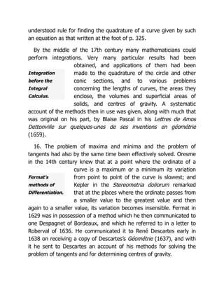
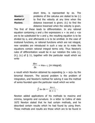
11. Fig. 7.
Fermat gave several examples of the application of his method;
among them was one in which he showed that he could differentiate
very complicated irrational functions. For such functions his method
was to begin by obtaining a rational equation. In rationalizing
equations Fermat, in other writings, used the device of introducing
new variables, but he did not use this device to simplify the process
of differentiation. Some of his results were published by Pierre
Hérigone in his Supplementum cursus mathematici (1642). His
communication to Descartes was not published in full until after his
death (Fermat, Opera varia, 1679). Methods similar to Fermat’s were
devised by René de Sluse (1652) for tangents, and by Johannes
Hudde (1658) for maxima and minima. Other methods for the
solution of the problem of tangents were devised by Roberval and
Torricelli, and published almost simultaneously in 1644. These
methods were founded upon the composition of motions, the theory
of which had been taught by Galileo (1638), and, less completely, by
Roberval (1636). Roberval and Torricelli could construct the tangents
of many curves, but they did not arrive at Fermat’s artifice. This
artifice is that which we have noted in § 10 as the fundamental
artifice of the infinitesimal calculus.
17. Among the comparatively few
mathematicians who before 1665 could
perform differentiations was Isaac
Barrow. In his book entitled Lectiones
opticae et geometricae, written
apparently in 1663, 1664, and published
in 1669, 1670, he gave a method of
tangents like that of Roberval and Torricelli, compounding two
velocities in the directions of the axes of x and y to obtain a
resultant along the tangent to a curve. In an appendix to this book

12. Barrow’s
Differential
Triangle.
Barrow’s
Inversion-
theorem.
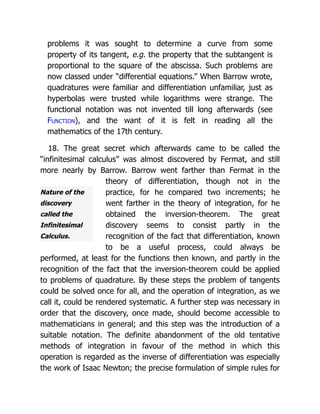
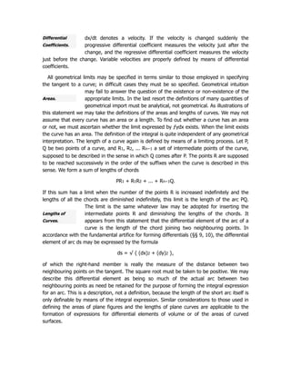
he gave another method which differs from
Fermat’s in the introduction of a differential
equivalent to our dy as well as dx. Two
neighbouring ordinates PM and QN of a curve
(fig. 7) are regarded as containing an indefinitely
small (indefinite parvum) arc, and PR is drawn parallel to the axis of
x. The tangent PT at P is regarded as identical with the secant PQ,
and the position of the tangent is determined by the similarity of the
triangles PTM, PQR. The increments QR, PR of the ordinate and
abscissa are denoted by a and e; and the ratio of a to e is
determined by substituting x + e for x and y + a for y in the
equation of the curve, rejecting all terms which are of order higher
than the first in a and e, and omitting the terms which do not
contain a or e. This process is equivalent to differentiation. Barrow
appears to have invented it himself, but to have put it into his book
at Newton’s request. The triangle PQR is sometimes called “Barrow’s
differential triangle.”
The reciprocal relation between differentiation and integration
(§ 6) was first observed explicitly by Barrow in the book cited
above. If the quadrature of a curve y = ƒ(x) is known, so that
the area up to the ordinate x is given by F(x), the curve y = F(x)
can be drawn, and Barrow showed that the
subtangent of this curve is measured by the
ratio of its ordinate to the ordinate of the
original curve. The curve y = F(x) is often
called the “quadratrix” of the original curve;
and the result has been called “Barrow’s inversion-theorem.” He
did not use it as we do for the determination of quadratures, or
indefinite integrals, but for the solution of problems of the kind
which were then called “inverse problems of tangents.” In these

13. Nature of the
discovery
called the
Infinitesimal
Calculus.
problems it was sought to determine a curve from some
property of its tangent, e.g. the property that the subtangent is
proportional to the square of the abscissa. Such problems are
now classed under “differential equations.” When Barrow wrote,
quadratures were familiar and differentiation unfamiliar, just as
hyperbolas were trusted while logarithms were strange. The
functional notation was not invented till long afterwards (see
Function), and the want of it is felt in reading all the
mathematics of the 17th century.
18. The great secret which afterwards came to be called the
“infinitesimal calculus” was almost discovered by Fermat, and still
more nearly by Barrow. Barrow went farther than Fermat in the
theory of differentiation, though not in the
practice, for he compared two increments; he
went farther in the theory of integration, for he
obtained the inversion-theorem. The great
discovery seems to consist partly in the
recognition of the fact that differentiation, known
to be a useful process, could always be
performed, at least for the functions then known, and partly in the
recognition of the fact that the inversion-theorem could be applied
to problems of quadrature. By these steps the problem of tangents
could be solved once for all, and the operation of integration, as we
call it, could be rendered systematic. A further step was necessary in
order that the discovery, once made, should become accessible to
mathematicians in general; and this step was the introduction of a
suitable notation. The definite abandonment of the old tentative
methods of integration in favour of the method in which this
operation is regarded as the inverse of differentiation was especially
the work of Isaac Newton; the precise formulation of simple rules for

14. Newton’s
investigations.
the process of differentiation in each special case, and the
introduction of the notation which has proved to be the best, were
especially the work of Gottfried Wilhelm Leibnitz. This statement
remains true although Newton invented a systematic notation, and
practised differentiation by rules equivalent to those of Leibnitz,
before Leibnitz had begun to work upon the subject, and Leibnitz
effected integrations by the method of recognizing differential
coefficients before he had had any opportunity of becoming
acquainted with Newton’s methods.
19. Newton was Barrow’s pupil, and he knew to start with in 1664
all that Barrow knew, and that was practically all that was known
about the subject at that time. His original thinking on the subject
dates from the year of the great plague (1665-
1666), and it issued in the invention of the
“Calculus of Fluxions,” the principles and methods
of which were developed by him in three tracts
entitled De analysi per aequationes numero terminorum infinitas,
Methodus fluxionum et serierum infinitarum, and De quadratura
curvarum. None of these was published until long after they were
written. The Analysis per aequationes was composed in 1666, but
not printed until 1711, when it was published by William Jones. The
Methodus fluxionum was composed in 1671 but not printed till 1736,
nine years after Newton’s death, when an English translation was
published by John Colson. In Horsley’s edition of Newton’s works it
bears the title Geometria analytica. The Quadratura appears to have
been composed in 1676, but was first printed in 1704 as an
appendix to Newton’s Opticks.
20. The tract De Analysi per aequationes ... was sent by
Newton to Barrow, who sent it to John Collins with a request

15. Newton’s
method of
Series.
that it might be made known. One way of making it known
would have been to print it in the Philosophical Transactions of
the Royal Society, but this course was not
adopted. Collins made a copy of the tract and
sent it to Lord Brouncker, but neither of them
brought it before the Royal Society. The tract
contains a general proof of Barrow’s
inversion-theorem which is the same in principle as that in § 6
above. In this proof and elsewhere in the tract a notation is
introduced for the momentary increment (momentum) of the
abscissa or area of a curve; this “moment” is evidently meant to
represent a moment of time, the abscissa representing time, and
it is effectively the same as our differential element—the thing
that Fermat had denoted by E, and Barrow by e, in the case of
the abscissa. Newton denoted the moment of the abscissa by o,
that of the area z by ov. He used the letter v for the ordinate y,
thus suggesting that his curve is a velocity-time graph such as
Galileo had used. Newton gave the formula for the area of a
curve v = xm(m ± −1) in the form z = xm+1/(m + 1). In the
proof he transformed this formula to the form zn = cn xp, where
n and p are positive integers, substituted x + o for x and z + ov
for z, and expanded by the binomial theorem for a positive
integral exponent, thus obtaining the relation
zn + nzn−1 ov + ... = cn (xp + pxp−1 o + ...),
from which he deduced the relation
nzn−1 v = cn pxp−1
by omitting the equal terms zn and cnxp and dividing the
remaining terms by o, tacitly putting o = 0 after division. This

16. relation is the same as v = xm. Newton pointed out that,
conversely, from the relation v = xm the relation z = xm+1 / (m +
1) follows. He applied his formula to the quadrature of curves
whose ordinates can be expressed as the sum of a finite number
of terms of the form axm; and gave examples of its application
to curves in which the ordinate is expressed by an infinite series,
using for this purpose the binomial theorem for negative and
fractional exponents, that is to say, the expansion of (1 + x)n in
an infinite series of powers of x. This theorem he had
discovered; but he did not in this tract state it in a general form
or give any proof of it. He pointed out, however, how it may be
used for the solution of equations by means of infinite series. He
observed also that all questions concerning lengths of curves,
volumes enclosed by surfaces, and centres of gravity, can be
formulated as problems of quadratures, and can thus be solved
either in finite terms or by means of infinite series. In the
Quadratura (1676) the method of integration which is founded
upon the inversion-theorem was carried out systematically.
Among other results there given is the quadrature of curves
expressed by equations of the form y = xn (a + bxm)p; this has
passed into text-books under the title “integration of binomial
differentials” (see § 49). Newton announced the result in letters
to Collins and Oldenburg of 1676.
21. In the Methodus fluxionum (1671) Newton introduced his
characteristic notation. He regarded variable quantities as
generated by the motion of a point, or line, or plane, and called
the generated quantity a “fluent” and its rate of generation a
“fluxion.” The fluxion of a fluent x is represented by x, and its
moment, or “infinitely” small increment accruing in an “infinitely”

17. Newton’s
method of
Fluxions.
short time, is represented by ẋo. The
problems of the calculus are stated to be (i.)
to find the velocity at any time when the
distance traversed is given; (ii.) to find the
distance traversed when the velocity is given.
The first of these leads to differentiation. In any rational
equation containing x and y the expressions x + ẋo and y +ẏo
are to be substituted for x and y, the resulting equation is to be
divided by o, and afterwards o is to be omitted. In the case of
irrational functions, or rational functions which are not integral,
new variables are introduced in such a way as to make the
equations contain rational integral terms only. Thus Newton’s
rules of differentiation would be in our notation the rules (i.),
(ii.), (v.) of § 11, together with the particular result which we
write
dxm
= mxm−1, (m integral).
dx
a result which Newton obtained by expanding (x = ẋo)m by the
binomial theorem. The second problem is the problem of
integration, and Newton’s method for solving it was the method
of series founded upon the particular result which we write
∫ xm dx =
xm+1
.
m + 1
Newton added applications of his methods to maxima and
minima, tangents and curvature. In a letter to Collins of date
1672 Newton stated that he had certain methods, and he
described certain results which he had found by using them.
These methods and results are those which are to be found in

18. Publication of
the Fluxional
Notation.
the Methodus fluxionum; but the letter makes no mention of
fluxions and fluents or of the characteristic notation. The rule for
tangents is said in the letter to be analogous to de Sluse’s, but
to be applicable to equations that contain irrational terms.
22. Newton gave the fluxional notation also in the tract De
Quadratura curvarum (1676), and he there added to it notation
for the higher differential coefficients and for indefinite integrals,
as we call them. Just as x, y, z, ... are fluents
of which ẋ, ẏ, ̇z, ... are the fluxions, so ẋ, ẏ, ̇z,
... can be treated as fluents of which the
fluxions may be denoted by ẍ, ̈y, ̈z,... In like
manner the fluxions of these may be denoted
by ẍ, ̈y, ̈z, ... and so on. Again x, y, z, ... may be regarded as
fluxions of which the fluents may be denoted by ́x, ́y, ́z, ... and
these again as fluxions of other quantities denoted by ̋x, ̋y, ̋z, ...
and so on. No use was made of the notation ́ x, ̋ x, ... in the
course of the tract. The first publication of the fluxional notation
was made by Wallis in the second edition of his Algebra (1693)
in the form of extracts from communications made to him by
Newton in 1692. In this account of the method the symbols 0, ẋ,
ẍ, ... occur, but not the symbols ́ x, ̋ x, .... Wallis’s treatise also
contains Newton’s formulation of the problems of the calculus in
the words Data aequatione fluentes quotcumque quantitates
involvente fluxiones invenire et vice versa (“an equation
containing any number of fluent quantities being given, to find
their fluxions and vice versa”). In the Philosophiae naturalis
principia mathematica (1687), commonly called the “Principia,”
the words “fluxion” and “moment” occur in a lemma in the
second book; but the notation which is characteristic of the
calculus of fluxions is nowhere used.

19. Retarded
Publication of
the method of
Fluxions.
23. It is difficult to account for the fragmentary manner of
publication of the Fluxional Calculus and for the long delays which
took place. At the time (1671) when Newton composed the
Methodus fluxionum he contemplated bringing
out an edition of Gerhard Kinckhuysen’s treatise
on algebra and prefixing his tract to this treatise.
In the same year his “Theory of Light and
Colours” was published in the Philosophical
Transactions, and the opposition which it excited
led to the abandonment of the project with regard to fluxions. In
1680 Collins sought the assistance of the Royal Society for the
publication of the tract, and this was granted in 1682. Yet it
remained unpublished. The reason is unknown; but it is known that
about 1679, 1680, Newton took up again the studies in natural
philosophy which he had intermitted for several years, and that in
1684 he wrote the tract De motu which was in some sense a first
draft of the Principia, and it may be conjectured that the fluxions
were held over until the Principia should be finished. There is also
reason to think that Newton had become dissatisfied with the
arguments about infinitesimals on which his calculus was based. In
the preface to the De quadratura curvarum (1704), in which he
describes this tract as something which he once wrote (“olim
scripsi”) he says that there is no necessity to introduce into the
method of fluxions any argument about infinitely small quantities;
and in the Principia (1687) he adopted instead of the method of
fluxions a new method, that of “Prime and Ultimate Ratios.” By the
aid of this method it is possible, as Newton knew, and as was
afterwards seen by others, to found the calculus of fluxions on an
irreproachable method of limits. For the purpose of explaining his
discoveries in dynamics and astronomy Newton used the method of

20. Leibnitz’s
course of
discovery.
limits only, without the notation of fluxions, and he presented all his
results and demonstrations in a geometrical form. There is no doubt
that he arrived at most of his theorems in the first instance by using
the method of fluxions. Further evidence of Newton’s dissatisfaction
with arguments about infinitely small quantities is furnished by his
tract Methodus diferentialis, published in 1711 by William Jones, in
which he laid the foundations of the “Calculus of Finite Differences.”
24. Leibnitz, unlike Newton, was practically a self-taught
mathematician. He seems to have been first attracted to
mathematics as a means of symbolical expression, and on the
occasion of his first visit to London, early in 1673,
he learnt about the doctrine of infinite series
which James Gregory, Nicolaus Mercator, Lord
Brouncker and others, besides Newton, had used
in their investigations. It appears that he did not
on this occasion become acquainted with Collins, or see Newton’s
Analysis per aequationes, but he purchased Barrow’s Lectiones. On
returning to Paris he made the acquaintance of Huygens, who
recommended him to read Descartes’ Géométrie. He also read
Pascal’s Lettres de Dettonville, Gregory of St Vincent’s Opus
geometricum, Cavalieri’s Indivisibles and the Synopsis geometrica of
Honoré Fabri, a book which is practically a commentary on Cavalieri;
it would never have had any importance but for the influence which
it had on Leibnitz’s thinking at this critical period. In August of this
year (1673) he was at work upon the problem of tangents, and he
appears to have made out the nature of the solution—the method
involved in Barrow’s differential triangle—for himself by the aid of a
diagram drawn by Pascal in a demonstration of the formula for the
area of a spherical surface. He saw that the problem of the relation
between the differences of neighbouring ordinates and the ordinates

21. themselves was the important problem, and then that the solution of
this problem was to be effected by quadratures. Unlike Newton, who
arrived at differentiation and tangents through integration and areas,
Leibnitz proceeded from tangents to quadratures. When he turned
his attention to quadratures and indivisibles, and realized the nature
of the process of finding areas by summing “infinitesimal”
rectangles, he proposed to replace the rectangles by triangles having
a common vertex, and obtained by this method the result which we
write
1⁄4π = 1 − 1⁄3 + 1⁄5 − 1⁄7 + ...
In 1674 he sent an account of his method, called “transmutation,”
along with this result to Huygens, and early in 1675 he sent it to
Henry Oldenburg, secretary of the Royal Society, with inquiries as to
Newton’s discoveries in regard to quadratures. In October of 1675
he had begun to devise a symbolical notation for quadratures,
starting from Cavalieri’s indivisibles. At first he proposed to use the
word omnia as an abbreviation for Cavalieri’s “sum of all the lines,”
thus writing omnia y for that which we write “∫ ydx,” but within a
day or two he wrote “∫ y”. He regarded the symbol “∫” as
representing an operation which raises the dimensions of the subject
of operation—a line becoming an area by the operation—and he
devised his symbol “d” to represent the inverse operation, by which
the dimensions are diminished. He observed that, whereas “∫”
represents “sum,” “d” represents “difference.” His notation appears
to have been practically settled before the end of 1675, for in
November he wrote ∫ ydy = ½ y2, just as we do now.
25. In July of 1676 Leibnitz received an answer to his inquiry in
regard to Newton’s methods in a letter written by Newton to
Oldenburg. In this letter Newton gave a general statement of the

22. Correspondenc
e of Newton
and Leibnitz.
binomial theorem and many results relating to
series. He stated that by means of such series he
could find areas and lengths of curves, centres of
gravity and volumes and surfaces of solids, but,
as this would take too long to describe, he would
illustrate it by examples. He gave no proofs. Leibnitz replied in
August, stating some results which he had obtained, and which, as it
seemed, could not be obtained easily by the method of series, and
he asked for further information. Newton replied in a long letter to
Oldenburg of the 24th of October 1676. In this letter he gave a
much fuller account of his binomial theorem and indicated a method
of proof. Further he gave a number of results relating to
quadratures; they were afterwards printed in the tract De quadratura
curvarum. He gave many other results relating to the computation of
natural logarithms and other calculations in which series could be
used. He gave a general statement, similar to that in the letter to
Collins, as to the kind of problems relating to tangents, maxima and
minima, &c., which he could solve by his method, but he concealed
his formulation of the calculus in an anagram of transposed letters.
The solution of the anagram was given eleven years later in the
Principia in the words we have quoted from Wallis’s Algebra. In
neither of the letters to Oldenburg does the characteristic notation of
the fluxional calculus occur, and the words “fluxion” and “fluent”
occur only in anagrams of transposed letters. The letter of October
1676 was not despatched until May 1677, and Leibnitz answered it in
June of that year. In October 1676 Leibnitz was in London, where he
made the acquaintance of Collins and read the Analysis per
aequationes, and it seems to have been supposed afterwards that
he then read Newton’s letter of October 1676, but he left London
before Oldenburg received this letter. In his answer of June 1677

23. Leibnitz’s
Differential
Calculus.
Leibnitz gave Newton a candid account of his differential calculus,
nearly in the form in which he afterwards published it, and explained
how he used it for quadratures and inverse problems of tangents.
Newton never replied.
26. In the Acta eruditorum of 1684 Leibnitz published a short
memoir entitled Nova methodus pro maximis et minimis, itemque
tangentibus, quae nec fractas nec irrationales quantitates moratur, et
singulare pro illis calculi genus. In this memoir the
differential dx of a variable x, considered as the
abscissa of a point of a curve, is said to be an
arbitrary quantity, and the differential dy of a
related variable y, considered as the ordinate of
the point, is defined as a quantity which has to dx the ratio of the
ordinate to the subtangent, and rules are given for operating with
differentials. These are the rules for forming the differential of a
constant, a sum (or difference), a product, a quotient, a power (or
root). They are equivalent to our rules (i.)-(iv.) of § 11 and the
particular result
d(xm) = mxm−1 dx.
The rule for a function of a function is not stated explicitly but is
illustrated by examples in which new variables are introduced, in
much the same way as in Newton’s Methodus fluxionum. In
connexion with the problem of maxima and minima, it is noted that
the differential of y is positive or negative according as y increases
or decreases when x increases, and the discrimination of maxima
from minima depends upon the sign of ddy, the differential of dy. In
connexion with the problem of tangents the differentials are said to
be proportional to the momentary increments of the abscissa and
ordinate. A tangent is defined as a line joining two “infinitely” near

24. Development of
the Calculus.
points of a curve, and the “infinitely” small distances (e.g., the
distance between the feet of the ordinates of such points) are said
to be expressible by means of the differentials (e.g., dx). The
method is illustrated by a few examples, and one example is given of
its application to “inverse problems of tangents.” Barrow’s inversion-
theorem and its application to quadratures are not mentioned. No
proofs are given, but it is stated that they can be obtained easily by
any one versed in such matters. The new methods in regard to
differentiation which were contained in this memoir were the use of
the second differential for the discrimination of maxima and minima,
and the introduction of new variables for the purpose of
differentiating complicated expressions. A greater novelty was the
use of a letter (d), not as a symbol for a number or magnitude, but
as a symbol of operation. None of these novelties account for the
far-reaching effect which this memoir has had upon the development
of mathematical analysis. This effect was a consequence of the
simplicity and directness with which the rules of differentiation were
stated. Whatever indistinctness might be felt to attach to the
symbols, the processes for solving problems of tangents and of
maxima and minima were reduced once for all to a definite routine.
27. This memoir was followed in 1686 by a second, entitled De
Geometria recondita et analysi indivisibilium atque infinitorum, in
which Leibnitz described the method of using his new differential
calculus for the problem of quadratures. This was
the first publication of the notation ∫ ydx. The
new method was called calculus summatorius.
The brothers Jacob (James) and Johann (John)
Bernoulli were able by 1690 to begin to make substantial
contributions to the development of the new calculus, and Leibnitz
adopted their word “integral” in 1695, they at the same time

25. Dispute
concerning
Priority.
adopting his symbol “∫.” In 1696 the marquis de l’Hospital published
the first treatise on the differential calculus with the title Analyse des
infiniment petits pour l’intelligence des lignes courbes. The few
references to fluxions in Newton’s Principia (1687) must have been
quite unintelligible to the mathematicians of the time, and the
publication of the fluxional notation and calculus by Wallis in 1693
was too late to be effective. Fluxions had been supplanted before
they were introduced.
The differential calculus and the integral calculus were rapidly
developed in the writings of Leibnitz and the Bernoullis. Leibnitz
(1695) was the first to differentiate a logarithm and an exponential,
and John Bernoulli was the first to recognize the property possessed
by an exponential (ax) of becoming infinitely great in comparison
with any power (xn) when x is increased indefinitely. Roger Cotes
(1722) was the first to differentiate a trigonometrical function. A
great development of infinitesimal methods took place through the
founding in 1696-1697 of the “Calculus of Variations” by the brothers
Bernoulli.
28. The famous dispute as to the priority of Newton and Leibnitz
in the invention of the calculus began in 1699 through the
publication by Nicolas Fatio de Duillier of a tract in which he stated
that Newton was not only the first, but by many
years the first inventor, and insinuated that
Leibnitz had stolen it. Leibnitz in his reply (Acta
Eruditorum, 1700) cited Newton’s letters and the
testimony which Newton had rendered to him in
the Principia as proofs of his independent authorship of the method.
Leibnitz was especially hurt at what he understood to be an
endorsement of Duillier’s attack by the Royal Society, but it was

26. explained to him that the apparent approval was an accident. The
dispute was ended for a time. On the publication of Newton’s tract
De quadratura curvarum, an anonymous review of it, written, as has
since been proved, by Leibnitz, appeared in the Acta Eruditorum,
1705. The anonymous reviewer said: “Instead of the Leibnitzian
differences Newton uses and always has used fluxions ... just as
Honoré Fabri in his Synopsis Geometrica substituted steps of
movements for the method of Cavalieri.” This passage, when it
became known in England, was understood not merely as belittling
Newton by comparing him with the obscure Fabri, but also as
implying that he had stolen his calculus of fluxions from Leibnitz.
Great indignation was aroused; and John Keill took occasion, in a
memoir on central forces which was printed in the Philosophical
Transactions for 1708, to affirm that Newton was without doubt the
first inventor of the calculus, and that Leibnitz had merely changed
the name and mode of notation. The memoir was published in 1710.
Leibnitz wrote in 1711 to the secretary of the Royal Society (Hans
Sloane) requiring Keill to retract his accusation. Leibnitz’s letter was
read at a meeting of the Royal Society, of which Newton was then
president, and Newton made to the society a statement of the
course of his invention of the fluxional calculus with the dates of
particular discoveries. Keill was requested by the society “to draw up
an account of the matter under dispute and set it in a just light.” In
his report Keill referred to Newton’s letters of 1676, and said that
Newton had there given so many indications of his method that it
could have been understood by a person of ordinary intelligence.
Leibnitz wrote to Sloane asking the society to stop these unjust
attacks of Keill, asserting that in the review in the Acta Eruditorum
no one had been injured but each had received his due, submitting
the matter to the equity of the Royal Society, and stating that he

27. was persuaded that Newton himself would do him justice. A
committee was appointed by the society to examine the documents
and furnish a report. Their report, presented in April 1712,
concluded as follows:
“The differential method is one and the same with the method
of fluxions, excepting the name and mode of notation; Mr
Leibnitz calling those quantities differences which Mr Newton
calls moments or fluxions, and marking them with the letter d, a
mark not used by Mr Newton. And therefore we take the proper
question to be, not who invented this or that method, but who
was the first inventor of the method; and we believe that those
who have reputed Mr Leibnitz the first inventor, knew little or
nothing of his correspondence with Mr Collins and Mr Oldenburg
long before; nor of Mr Newton’s having that method above
fifteen years before Mr. Leibnitz began to publish it in the Acta
Eruditorum of Leipzig. For which reasons we reckon Mr Newton
the first inventor, and are of opinion that Mr Keill, in asserting
the same, has been no ways injurious to Mr Leibnitz.”
The report with the letters and other documents was printed
(1712) under the title Commercium Epistolicum D. Johannis Collins
et aliorum de analysi promota, jussu Societatis Regiae in lucem
editum, not at first for publication. An account of the contents of the
Commercium Epistolicum was printed in the Philosophical
Transactions for 1715. A second edition of the Commercium
Epistolicum was published in 1722. The dispute was continued for
many years after the death of Leibnitz in 1716. To translate the
words of Moritz Cantor, it “redounded to the discredit of all
concerned.”

28. British and
Continental
Schools of
Mathematics.
29. One lamentable consequence of the dispute was a severance
of British methods from continental ones. In Great Britain it became
a point of honour to use fluxions and other Newtonian methods,
while on the continent the notation of Leibnitz
was universally adopted. This severance did not
at first prevent a great advance in mathematics in
Great Britain. So long as attention was directed to
problems in which there is but one independent
variable (the time, or the abscissa of a point of a
curve), and all the other variables depend upon this one, the
fluxional notation could be used as well as the differential and
integral notation, though perhaps not quite so easily. Up to about
the middle of the 18th century important discoveries continued to be
made by the use of the method of fluxions. It was the introduction
of partial differentiation by Leonhard Euler (1734) and Alexis Claude
Clairaut (1739), and the developments which followed upon the
systematic use of partial differential coefficients, which led to Great
Britain being left behind; and it was not until after the reintroduction
of continental methods into England by Sir John Herschel, George
Peacock and Charles Babbage in 1815 that British mathematics
began to flourish again. The exclusion of continental mathematics
from Great Britain was not accompanied by any exclusion of British
mathematics from the continent. The discoveries of Brook Taylor and
Colin Maclaurin were absorbed into the rapidly growing continental
analysis, and the more precise conceptions reached through a critical
scrutiny of the true nature of Newton’s fluxions and moments
stimulated a like scrutiny of the basis of the method of differentials.
30. This method had met with opposition from the first. Christiaan
Huygens, whose opinion carried more weight than that of any other
scientific man of the day, declared that the employment of

29. Oppositions to
the calculus.
The “Analyst”
controversy.
differentials was unnecessary, and that Leibnitz’s
second differential was meaningless (1691). A
Dutch physician named Bernhard Nieuwentijt
attacked the method on account of the use of
quantities which are at one stage of the process treated as
somethings and at a later stage as nothings, and he was especially
severe in commenting upon the second and higher differentials
(1694, 1695). Other attacks were made by Michel Rolle (1701), but
they were directed rather against matters of detail than against the
general principles. The fact is that, although Leibnitz in his answers
to Nieuwentijt (1695), and to Rolle (1702), indicated that the
processes of the calculus could be justified by the methods of the
ancient geometry, he never expressed himself very clearly on the
subject of differentials, and he conveyed, probably without intending
it, the impression that the calculus leads to correct results by
compensation of errors. In England the method of fluxions had to
face similar attacks. George Berkeley, bishop and philosopher, wrote
in 1734 a tract entitled The Analyst; or a Discourse addressed to an
Infidel Mathematician, in which he proposed to destroy the
presumption that the opinions of mathematicians
in matters of faith are likely to be more
trustworthy than those of divines, by contending
that in the much vaunted fluxional calculus there
are mysteries which are accepted unquestioningly by the
mathematicians, but are incapable of logical demonstration.
Berkeley’s criticism was levelled against all infinitesimals, that is to
say, all quantities vaguely conceived as in some intermediate state
between nullity and finiteness, as he took Newton’s moments to be
conceived. The tract occasioned a controversy which had the
important consequence of making it plain that all arguments about

30. infinitesimals must be given up, and the calculus must be founded
on the method of limits. During the controversy Benjamin Robins
gave an exceedingly clear explanation of Newton’s theories of
fluxions and of prime and ultimate ratios regarded as theories of
limits. In this explanation he pointed out that Newton’s moment
(Leibnitz’s “differential”) is to be regarded as so much of the actual
difference between two neighbouring values of a variable as is
needful for the formation of the fluxion (or differential coefficient)
(see G. A. Gibson, “The Analyst Controversy,” Proc. Math. Soc.,
Edinburgh, xvii., 1899). Colin Maclaurin published in 1742 a Treatise
of Fluxions, in which he reduced the whole theory to a theory of
limits, and demonstrated it by the method of Archimedes. This
notion was gradually transferred to the continental mathematicians.
Leonhard Euler in his Institutiones Calculi differentialis (1755) was
reduced to the position of one who asserts that all differentials are
zero, but, as the product of zero and any finite quantity is zero, the
ratio of two zeros can be a finite quantity which it is the business of
the calculus to determine. Jean le Rond d’Alembert in the
Encyclopédie méthodique (1755, 2nd ed. 1784) declared that
differentials were unnecessary, and that Leibnitz’s calculus was a
calculus of mutually compensating errors, while Newton’s method
was entirely rigorous. D’Alembert’s opinion of Leibnitz’s calculus was
expressed also by Lazare N. M. Carnot in his Réflexions sur la
métaphysique du calcul infinitésimal (1799) and by Joseph Louis de
la Grange (generally called Lagrange) in writings from 1760
onwards. Lagrange proposed in his Théorie des fonctions analytiques
(1797) to found the whole of the calculus on the theory of series. It
was not until 1823 that a treatise on the differential calculus founded
upon the method of limits was published. The treatise was the
Résumé des leçons ... sur le calcul infinitésimal of Augustin Louis

31. Cauchy’s
method of
limits.
Arithmetical
basis of
modern
analysis.
Cauchy. Since that time it has been understood
that the use of the phrase “infinitely small” in any
mathematical argument is a figurative mode of
expression pointing to a limiting process. In the
opinion of many eminent mathematicians such
modes of expression are confusing to students, but in treatises on
the calculus the traditional modes of expression are still largely
adopted.
31. Defective modes of expression did not hinder constructive
work. It was the great merit of Leibnitz’s symbolism that a
mathematician who used it knew what was to be done in order to
formulate any problem analytically, even though
he might not be absolutely clear as to the proper
interpretation of the symbols, or able to render a
satisfactory account of them. While new and
varied results were promptly obtained by using
them, a long time elapsed before the theory of
them was placed on a sound basis. Even after Cauchy had
formulated his theory much remained to be done, both in the rapidly
growing department of complex variables, and in the regions opened
up by the theory of expansions in trigonometric series. In both
directions it was seen that rigorous demonstration demanded
greater precision in regard to fundamental notions, and the
requirement of precision led to a gradual shifting of the basis of
analysis from geometrical intuition to arithmetical law. A sketch of
the outcome of this movement—the “arithmetization of analysis,” as
it has been called—will be found in Function. Its general tendency
has been to show that many theories and processes, at first
accepted as of general validity, are liable to exceptions, and much of
the work of the analysts of the latter half of the 19th century was

32. Fig. 8.
directed to discovering the most general conditions in which
particular processes, frequently but not universally applicable, can be
used without scruple.
III. Outlines of the Infinitesimal Calculus.
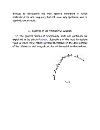
32. The general notions of functionality, limits and continuity are
explained in the article Function. Illustrations of the more immediate
ways in which these notions present themselves in the development
of the differential and integral calculus will be useful in what follows.

33. Geometrical
limits.
Tangents.
Progressive
and Regressive
33. Let y be given as a function of x, or, more generally, let x and y be given as functions
of a variable t. The first of these cases is included in the second by putting x = t. If certain
conditions are satisfied the aggregate of the points determined by the
functional relations form a curve. The first condition is that the
aggregate of the values of t to which values of x and y correspond must
be continuous, or, in other words, that these values must consist of all
real numbers, or of all those real numbers which lie between assigned extreme numbers.
When this condition is satisfied the points are “ordered,” and their order is determined by
the order of the numbers t, supposed to be arranged in order of increasing or decreasing
magnitude; also there are two senses of description of the curve, according as t is taken to
increase or to diminish. The second condition is that the aggregate of the points which are
determined by the functional relations must be “continuous.” This condition means that, if
any point P determined by a value of t is taken, and any distance δ, however small, is
chosen, it is possible to find two points Q, Q′ of the aggregate which are such that (i.) P is
between Q and Q′, (ii.) if R, R′ are any points between Q and Q′ the distance RR′ is less
than δ. The meaning of the word “between” in this statement is fixed by the ordering of
the points. Sometimes additional conditions are imposed upon the functional relations
before they are regarded as defining a curve. An aggregate of points which satisfies the
two conditions stated above is sometimes called a “Jordan curve.” It by no means follows
that every curve of this kind has a tangent. In order that the curve may
have a tangent at P it is necessary that, if any angle α, however small, is
specified, a distance δ can be found such that when P is between Q and
Q′, and PQ and PQ′ are less than δ, the angle RPR′ is less than α for all pairs of points R, R′
which are between P and Q, or between P and Q′ (fig. 8). When this condition is satisfied y
is a function of x which has a differential coefficient. The only way of finding out whether
this condition is satisfied or not is to attempt to form the differential coefficient. If the
quotient of differences Δy/Δx has a limit when Δx tends to zero, y is a differentiable
function of x, and the limit in question is the differential coefficient. The derived function, or
differential coefficient, of a function ƒ(x) is always defined by the formula
ƒ′(x) =
dƒ(x)
= lim.h=0
ƒ(x + h) − ƒ(x)
.
dx h
Rules for the formation of differential coefficients in particular cases have been given in §
11 above. The definition of a differential coefficient, and the rules of differentiation are
quite independent of any geometrical interpretation, such as that concerning tangents to a
curve, and the tangent to a curve is properly defined by means of the differential coefficient
of a function, not the differential coefficient by means of the tangent.
It may happen that the limit employed in defining the differential coefficient has one
value when h approaches zero through positive values, and a different value when h
approaches zero through negative values. The two limits are then called
the “progressive” and “regressive” differential coefficients. In
applications to dynamics, when x denotes a coordinate and t the time,

34. Differential
Coefficients.
Areas.
Lengths of
Curves.
dx/dt denotes a velocity. If the velocity is changed suddenly the
progressive differential coefficient measures the velocity just after the
change, and the regressive differential coefficient measures the velocity
just before the change. Variable velocities are properly defined by means of differential
coefficients.
All geometrical limits may be specified in terms similar to those employed in specifying
the tangent to a curve; in difficult cases they must be so specified. Geometrical intuition
may fail to answer the question of the existence or non-existence of the
appropriate limits. In the last resort the definitions of many quantities of
geometrical import must be analytical, not geometrical. As illustrations of
this statement we may take the definitions of the areas and lengths of curves. We may not
assume that every curve has an area or a length. To find out whether a curve has an area
or not, we must ascertain whether the limit expressed by ƒydx exists. When the limit exists
the curve has an area. The definition of the integral is quite independent of any geometrical
interpretation. The length of a curve again is defined by means of a limiting process. Let P,
Q be two points of a curve, and R1, R2, ... Rn−1 a set of intermediate points of the curve,
supposed to be described in the sense in which Q comes after P. The points R are supposed
to be reached successively in the order of the suffixes when the curve is described in this
sense. We form a sum of lengths of chords
PR1 + R1R2 + ... + Rn−1Q.
If this sum has a limit when the number of the points R is increased indefinitely and the
lengths of all the chords are diminished indefinitely, this limit is the length of the arc PQ.
The limit is the same whatever law may be adopted for inserting the
intermediate points R and diminishing the lengths of the chords. It
appears from this statement that the differential element of the arc of a
curve is the length of the chord joining two neighbouring points. In
accordance with the fundamental artifice for forming differentials (§§ 9, 10), the differential
element of arc ds may be expressed by the formula
ds = √ { (dx)2 + (dy)2 },
of which the right-hand member is really the measure of the distance between two
neighbouring points on the tangent. The square root must be taken to be positive. We may
describe this differential element as being so much of the actual arc between two
neighbouring points as need be retained for the purpose of forming the integral expression
for an arc. This is a description, not a definition, because the length of the short arc itself is
only definable by means of the integral expression. Similar considerations to those used in
defining the areas of plane figures and the lengths of plane curves are applicable to the
formation of expressions for differential elements of volume or of the areas of curved
surfaces.

35. Constants of
Integration.
Higher
Differential
Coefficients.
34. In regard to differential coefficients it is an important theorem
that, if the derived function ƒ′(x) vanishes at all points of an interval, the
function ƒ(x) is constant in the interval. It follows that, if two functions
have the same derived function they can only differ by a constant.
Conversely, indefinite integrals are indeterminate to the extent of an additive constant.
35. The differential coefficient dy/dx, or the derived function ƒ′(x), is itself a function of
x, and its differential coefficient is denoted by ƒ″(x) or d2y/dx2. In the
second of these notations d/dx is regarded as the symbol of an
operation, that of differentiation with respect to x, and the index 2
means that the operation is repeated. In like manner we may express
the results of n successive differentiations by ƒ(n)(x) or by dny/dxn.
When the second differential coefficient exists, or the first is differentiable, we have the
relation
ƒ″(x) = lim.h=0
ƒ(x + h) − 2ƒ(x) + ƒ(x − h)
.
h2
(i.)
The limit expressed by the right-hand member of this equation may exist in cases in which
ƒ′(x) does not exist or is not differentiable. The result that, when the limit here expressed
can be shown to vanish at all points of an interval, then ƒ(x) must be a linear function of x
in the interval, is important.
The relation (i.) is a particular case of the more general relation
ƒ(n)(x) = lim.h=0 h−n [ ƒ(x + nh) − nf {(x + (n − 1) h }
+
n (n − 1)
ƒ {x + (n − 2) h } − ... + (−1)n ƒ(x) ].
2! (ii.)
As in the case of relation (i.) the limit expressed by the right-hand member may exist
although some or all of the derived functions ƒ′(x), ƒ″(x), ... ƒ(n−1)(x) do not exist.
Corresponding to the rule iii. of § 11 we have the rule for forming the nth differential
coefficient of a product in the form
dn(uv)
= u
dnv
+ n
du dn−1v
+
n(n − 1) d2u dn−2v
+ ... +
dnu
v,
dxn dxn dx dxn−1 1·2 dx2 dxn−2 dxn
where the coefficients are those of the expansion of (1 + x)n in powers of x (n being a
positive integer). The rule is due to Leibnitz, (1695).
Differentials of higher orders may be introduced in the same way as the differential of
the first order. In general when y = ƒ(x), the nth differential dny is defined by the equation
dny = ƒ(n) (x) (dx)n,
in which dx is the (arbitrary) differential of x.

36. Symbols of
operation.
Fig. 9.
Theorem of
Intermediate
Value.
When d/dx is regarded as a single symbol of operation the symbol ƒ ... dx represents the
inverse operation. If the former is denoted by D, the latter may be denoted by D−1. Dn
means that the operation D is to be performed n times in succession;
D−n that the operation of forming the indefinite integral is to be
performed n times in succession. Leibnitz’s course of thought (§ 24)
naturally led him to inquire after an interpretation of Dn. where n is not
an integer. For an account of the researches to which this inquiry gave rise, reference may
be made to the article by A. Voss in Ency. d. math. Wiss. Bd. ii. A, 2 (Leipzig, 1889). The
matter is referred to as “fractional” or “generalized” differentiation.
36. After the formation of differential coefficients the most
important theorem of the differential calculus is the theorem of
intermediate value (“theorem of mean value,”
“theorem of finite increments,” “Rolle’s
theorem,” are other names for it). This
theorem may be explained as follows: Let A,
B be two points of a curve y = ƒ(x) (fig. 9).
Then there is a point P between A and B at which the tangent is parallel to the secant AB.
This theorem is expressed analytically in the statement that if ƒ′(x) is continuous between
a and b, there is a value x1 of x between a and b which has the property expressed by the
equation
ƒ(b) − ƒ(a)
= ƒ′(x1).
b − a (i.)
The value x1 can be expressed in the form a + θ(b − a) where θ is a number between 0
and 1.
A slightly more general theorem was given by Cauchy (1823) to the effect that, if ƒ′(x)
and F′(x) are continuous between x = a and x = b, then there is a number θ between 0
and 1 which has the property expressed by the equation
F(b) − F(a)
=
F′ {a + θ(b − a) }
.
ƒ(b) − ƒ(a) ƒ′ {a + θ(b − a) }
The theorem expressed by the relation (i.) was first noted by Rolle (1690) for the case
where ƒ(x) is a rational integral function which vanishes when x = a and also when x = b.
The general theorem was given by Lagrange (1797). Its fundamental importance was first
recognized by Cauchy (1823). It may be observed here that the theorem of integral
calculus expressed by the equation
F(b) − F(a) = ∫b
a F′(x) dx
follows at once from the definition of an integral and the theorem of intermediate value.

37. Taylor’s
Theorem.
The theorem of intermediate value may be generalized in the statement that, if ƒ(x) and
all its differential coefficients up to the nth inclusive are continuous in the interval between
x = a and x = b, then there is a number θ between 0 and 1 which has the property
expressed by the equation
ƒ(b) = ƒ(a) + (b − a) ƒ′(a) +
(b − a)2
ƒ″(a) + ... +
(b − a)n−1
ƒ(n−1)(a)
2! (n − 1)!
+
(b − a)n
ƒ(n) {a + θ (b − a) }.
n! (ii.)
37. This theorem provides a means for computing the values of a function at points near
to an assigned point when the value of the function and its differential coefficients at the
assigned point are known. The function is expressed by a terminated
series, and, when the remainder tends to zero as n increases, it may be
transformed into an infinite series. The theorem was first given by Brook
Taylor in his Methodus Incrementorum (1717) as a corollary to a
theorem concerning finite differences. Taylor gave the expression for ƒ(x + z) in terms of
ƒ(x), ƒ′(x), ... as an infinite series proceeding by powers of z. His notation was that
appropriate to the method of fluxions which he used. This rule for expressing a function as
an infinite series is known as Taylor’s theorem. The relation (i.), in which the remainder
after n terms is put in evidence, was first obtained by Lagrange (1797). Another form of
the remainder was given by Cauchy (1823) viz.,
(b − a)n
(1 − θ)n−1 ƒn {a + θ(b − a) }.
(n − 1)!
The conditions of validity of Taylor’s expansion in an infinite series have been investigated
very completely by A. Pringsheim (Math. Ann. Bd. xliv., 1894). It is not sufficient that the
function and all its differential coefficients should be finite at x = a; there must be a
neighbourhood of a within which Cauchy’s form of the remainder tends to zero as n
increases (cf. Function).
An example of the necessity of this condition is afforded by the function f(x) which is
given by the equation
ƒ(x) =
1
+ Σn=∞
n=1
(−1)n 1
.
1 + x2 n! 1 + 32n x2
(i.)
The sum of the series
ƒ(0) + xƒ′(0) +
x2
ƒ″(0)+ ...
2! (ii.)
is the same as that of the series
e−1 − x2 e−32 + x4 e−34 − ...

38. Expansions in
power series.
It is easy to prove that this is less than e−1 when x lies between 0 and 1, and also that f(x)
is greater than e−l when x = 1/√3. Hence the sum of the series (i.) is not equal to the sum
of the series (ii.).
The particular case of Taylor’s theorem in which a = 0 is often called Maclaurin’s
theorem, because it was first explicitly stated by Colin Maclaurin in his Treatise of Fluxions
(1742). Maclaurin like Taylor worked exclusively with the fluxional calculus.
Examples of expansions in series had been known for some time. The series for log (1 +
x) was obtained by Nicolaus Mercator (1668) by expanding (1 + x)−1 by the method of
algebraic division, and integrating the series term by term. He regarded
his result as a “quadrature of the hyperbola.” Newton (1669) obtained
the expansion of sin−1x by expanding (l − x2)−1/2 by the binomial
theorem and integrating the series term by term. James Gregory (1671)
gave the series for tan−1x. Newton also obtained the series for sin x, cos x, and ex by
reversion of series (1669). The symbol e for the base of the Napierian logarithms was
introduced by Euler (1739). All these series can be obtained at once by Taylor’s theorem.
James Gregory found also the first few terms of the series for tan x and sec x; the terms of
these series may be found successively by Taylor’s theorem, but the numerical coefficient of
the general term cannot be obtained in this way.
Taylor’s theorem for the expansion of a function in a power series was the basis of
Lagrange’s theory of functions, and it is fundamental also in the theory of analytic functions
of a complex variable as developed later by Karl Weierstrass. It has also numerous
applications to problems of maxima and minima and to analytical geometry. These matters
are treated in the appropriate articles.
The forms of the coefficients in the series for tan x and sec x can be expressed most
simply in terms of a set of numbers introduced by James Bernoulli in his treatise on
probability entitled Ars Conjectandi (1713). These numbers B1, B2, ... called Bernoulli’s
numbers, are the coefficients so denoted in the formula
x
= 1 −
x
+
B1
x2 −
B2
x4 +
B3
x6 − ...,
ex − 1 2 2! 4! 6!
and they are connected with the sums of powers of the reciprocals of the natural numbers
by equations of the type
Bn =
(2n)!
(
1
+
1
+
1
+ ... ).
22n−1 π2n 12n 22n 32n
The function
xm −
m
xm−1 +
m·m − 1
B1 xm−2 − ...
2 2!

39. Welcome to our website – the perfect destination for book lovers and
knowledge seekers. We believe that every book holds a new world,
offering opportunities for learning, discovery, and personal growth.
That’s why we are dedicated to bringing you a diverse collection of
books, ranging from classic literature and specialized publications to
self-development guides and children's books.
More than just a book-buying platform, we strive to be a bridge
connecting you with timeless cultural and intellectual values. With an
elegant, user-friendly interface and a smart search system, you can
quickly find the books that best suit your interests. Additionally,
our special promotions and home delivery services help you save time
and fully enjoy the joy of reading.
Join us on a journey of knowledge exploration, passion nurturing, and
personal growth every day!
testbankfan.com