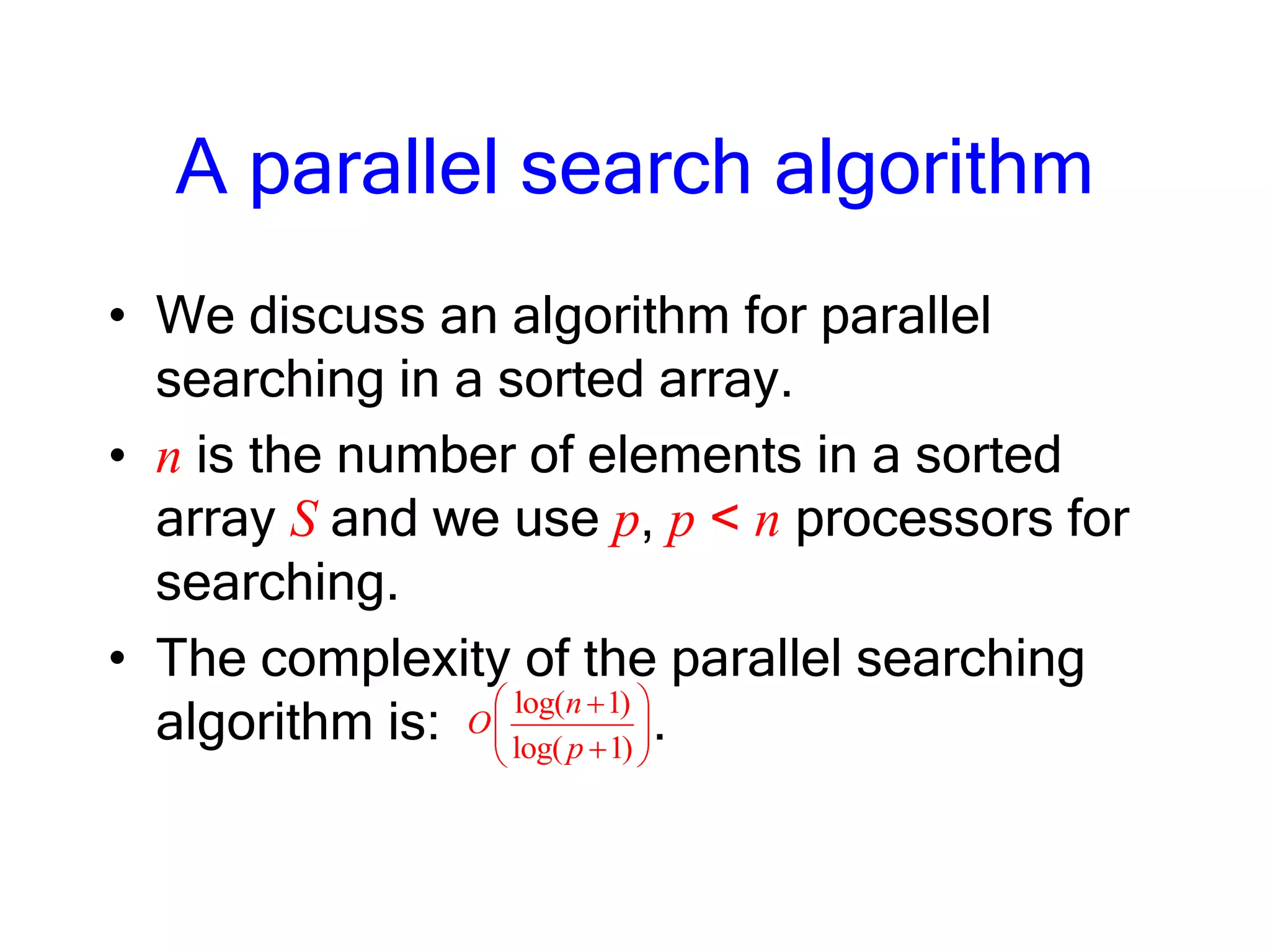
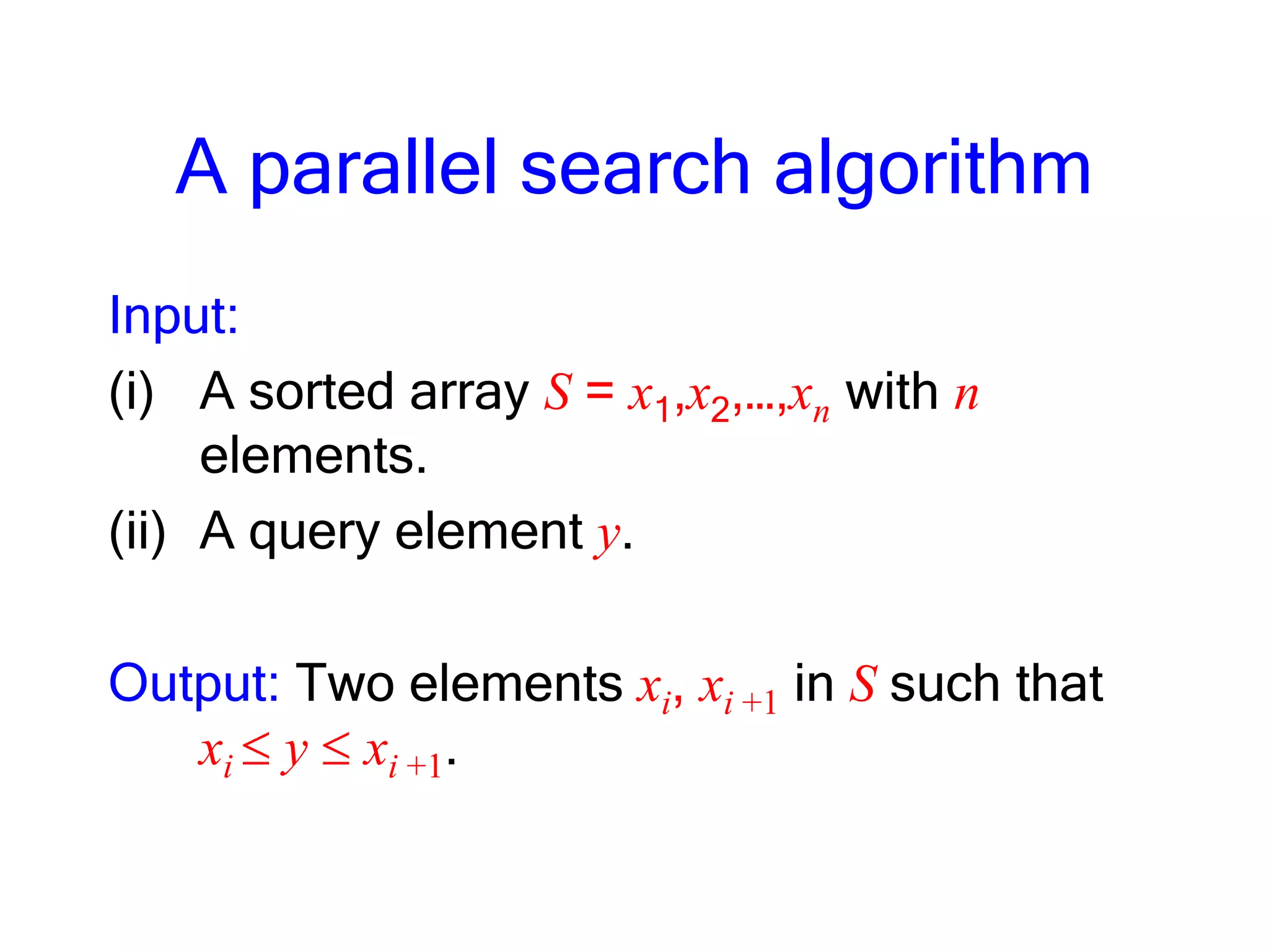
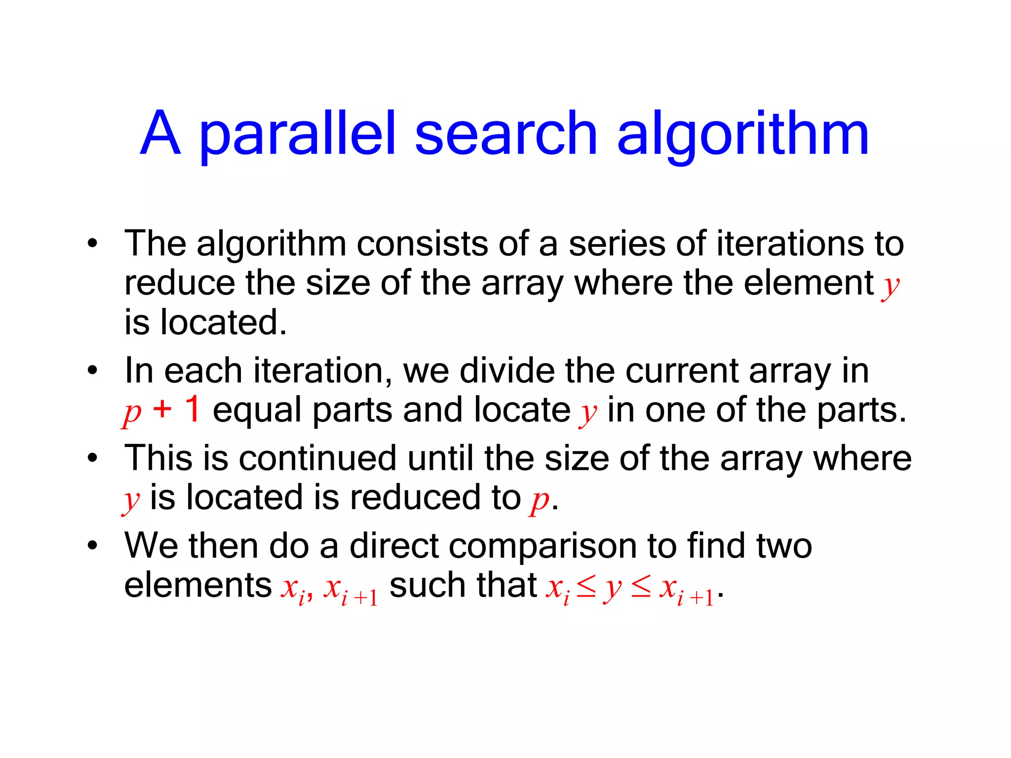
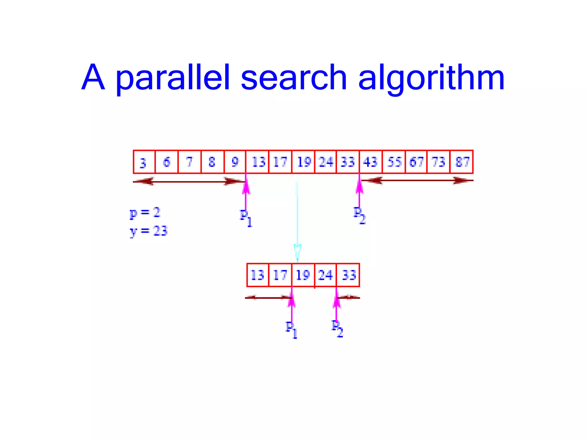
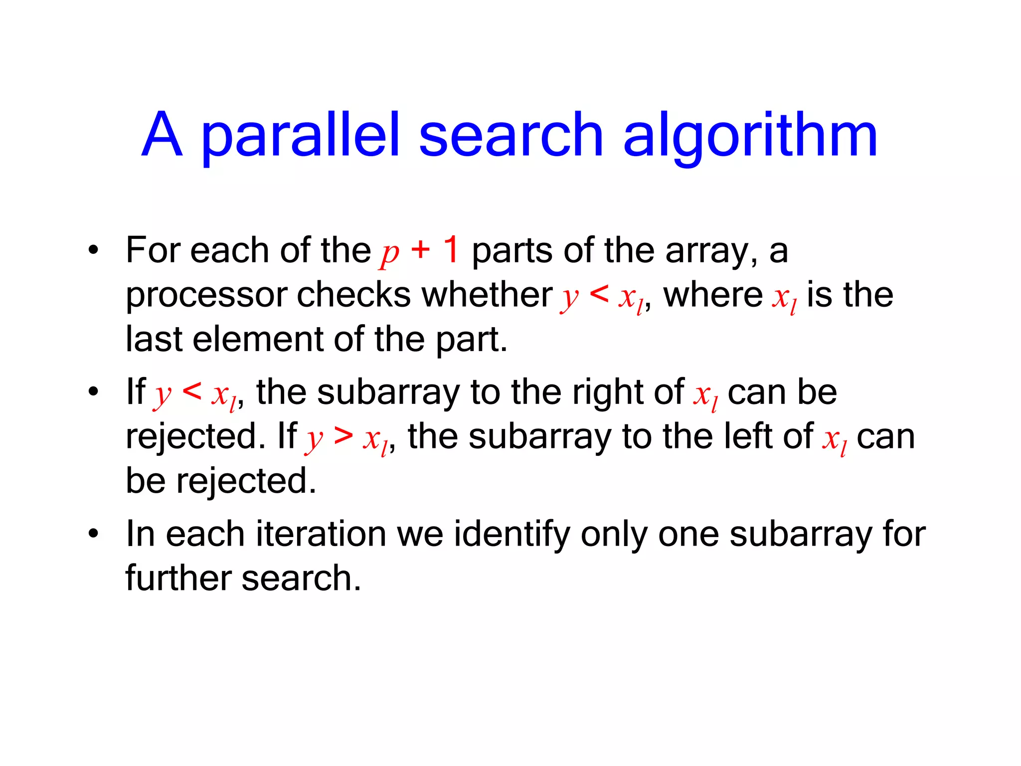
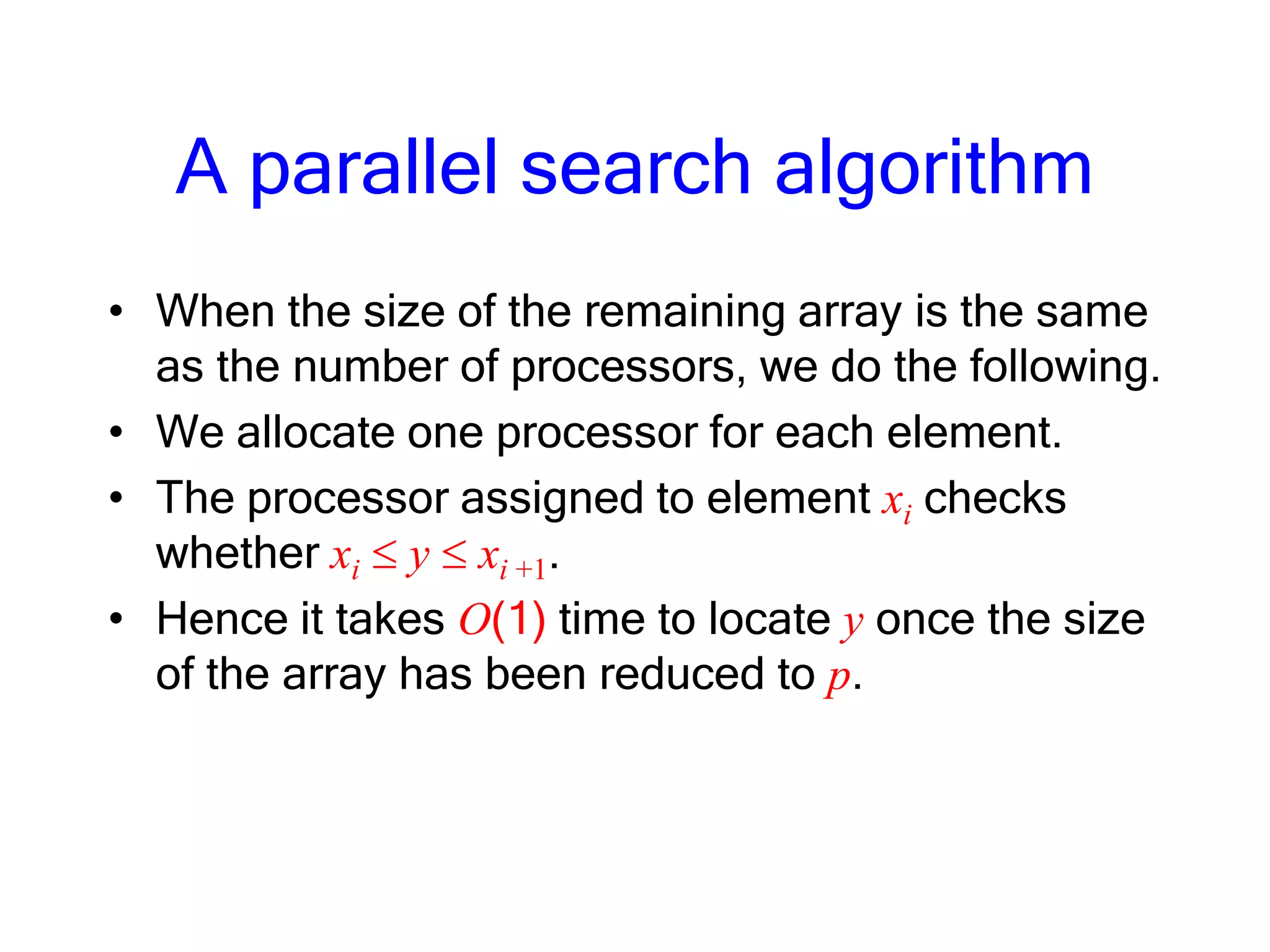
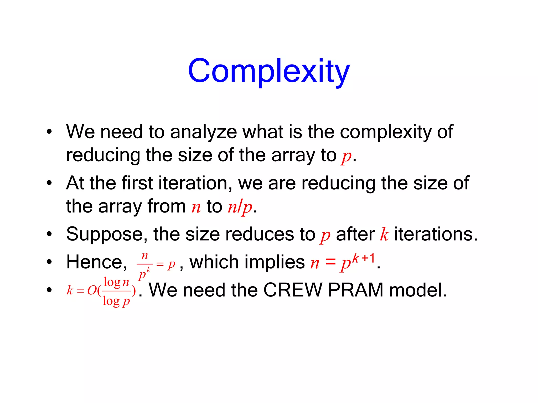
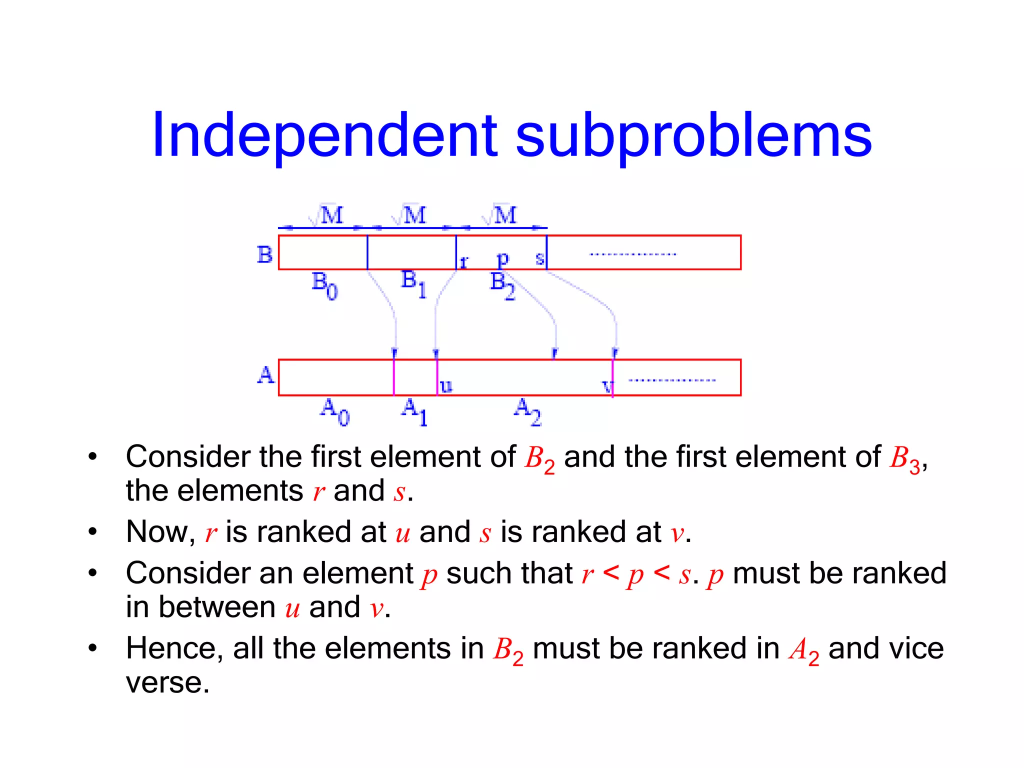
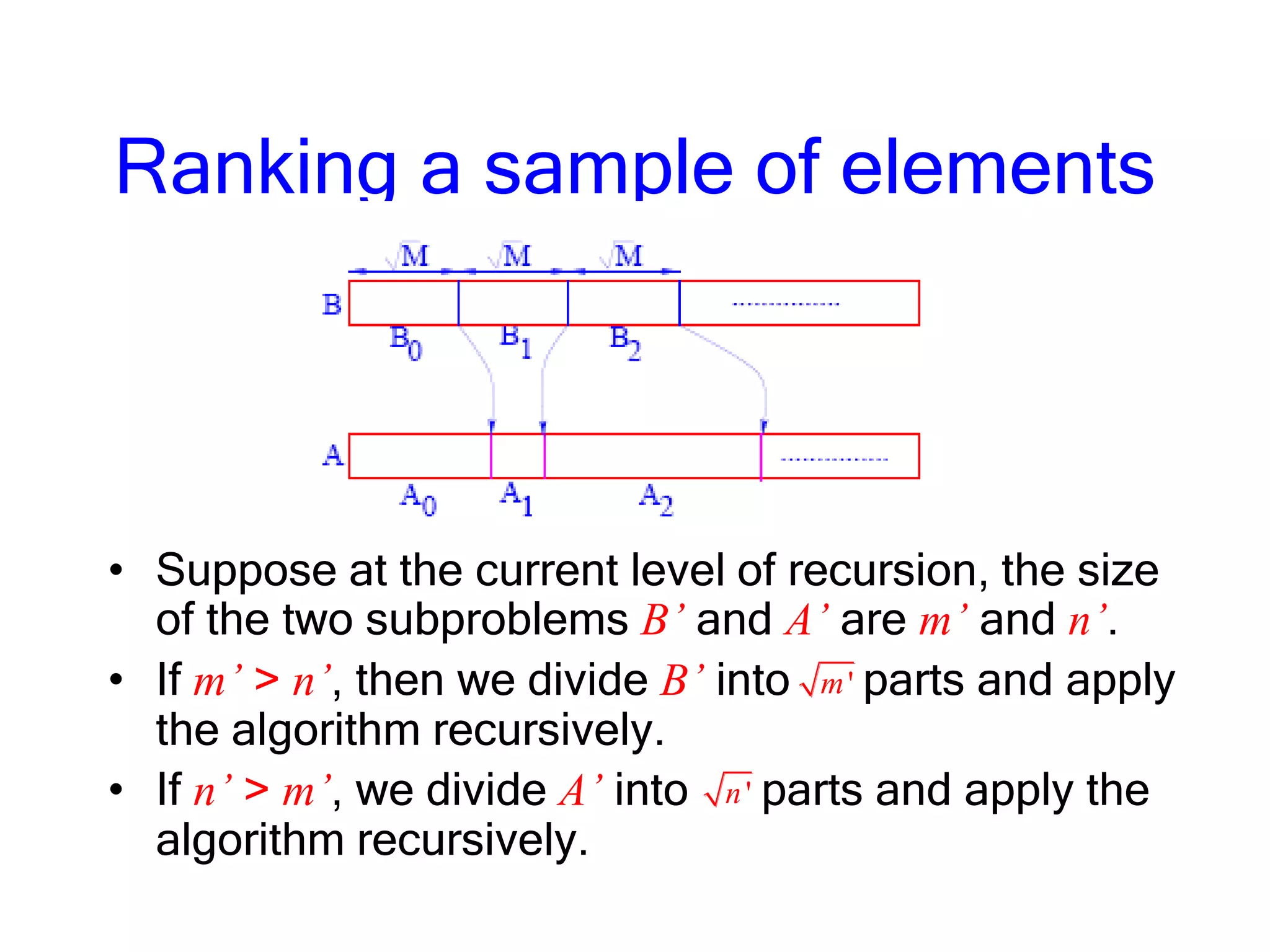
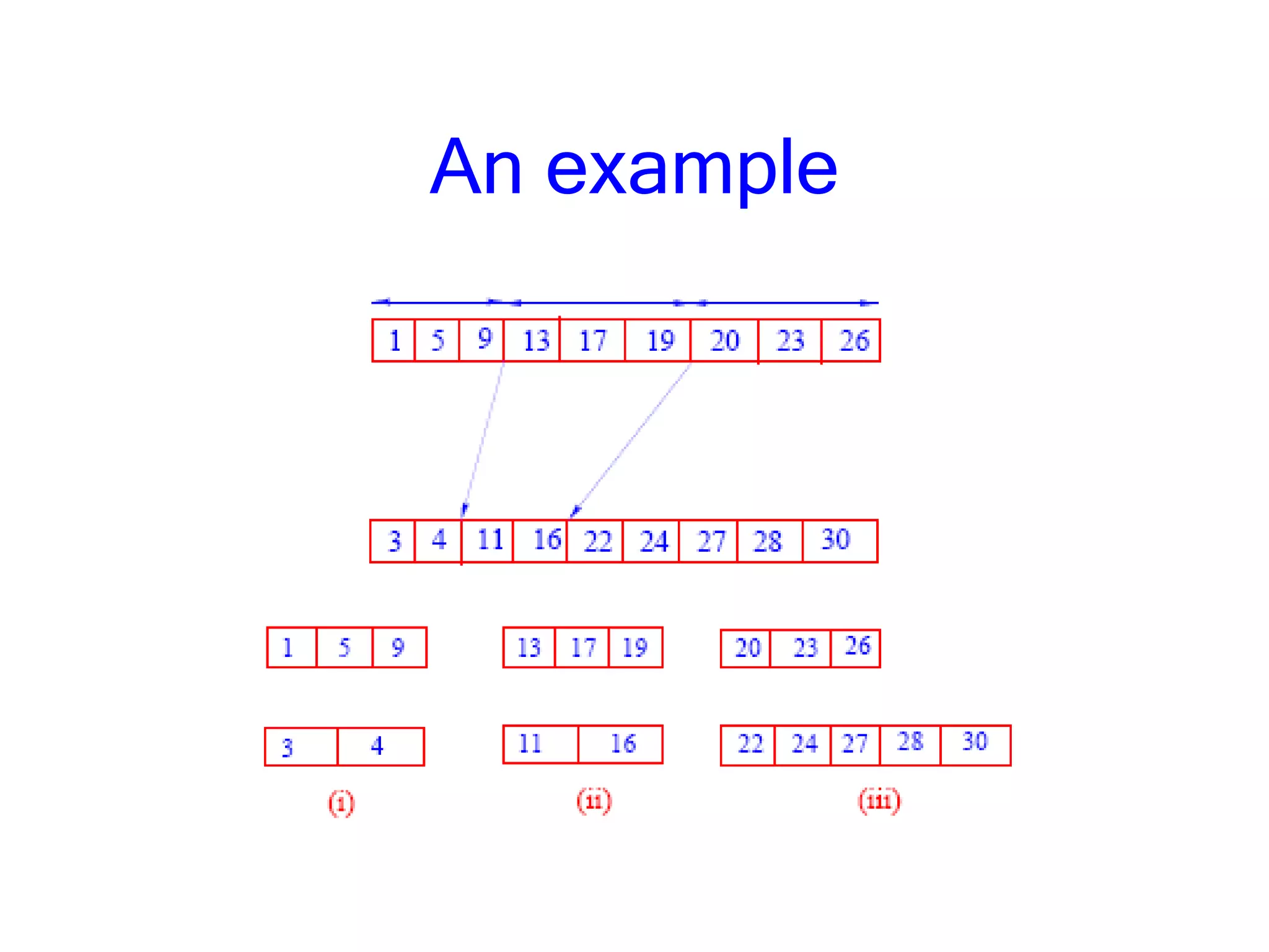
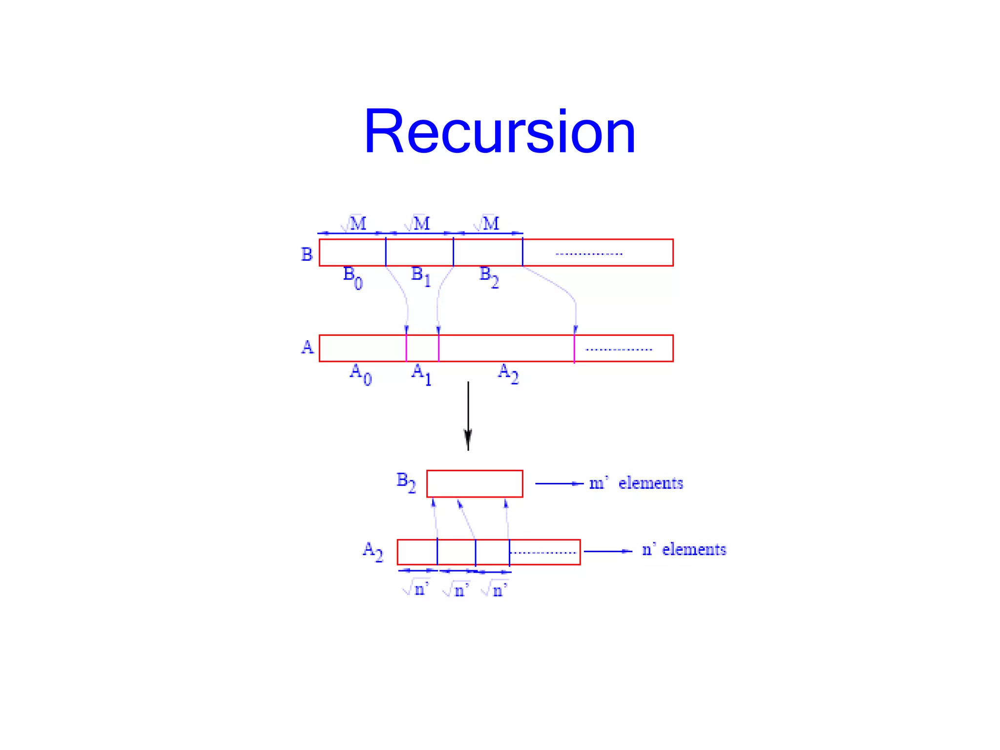
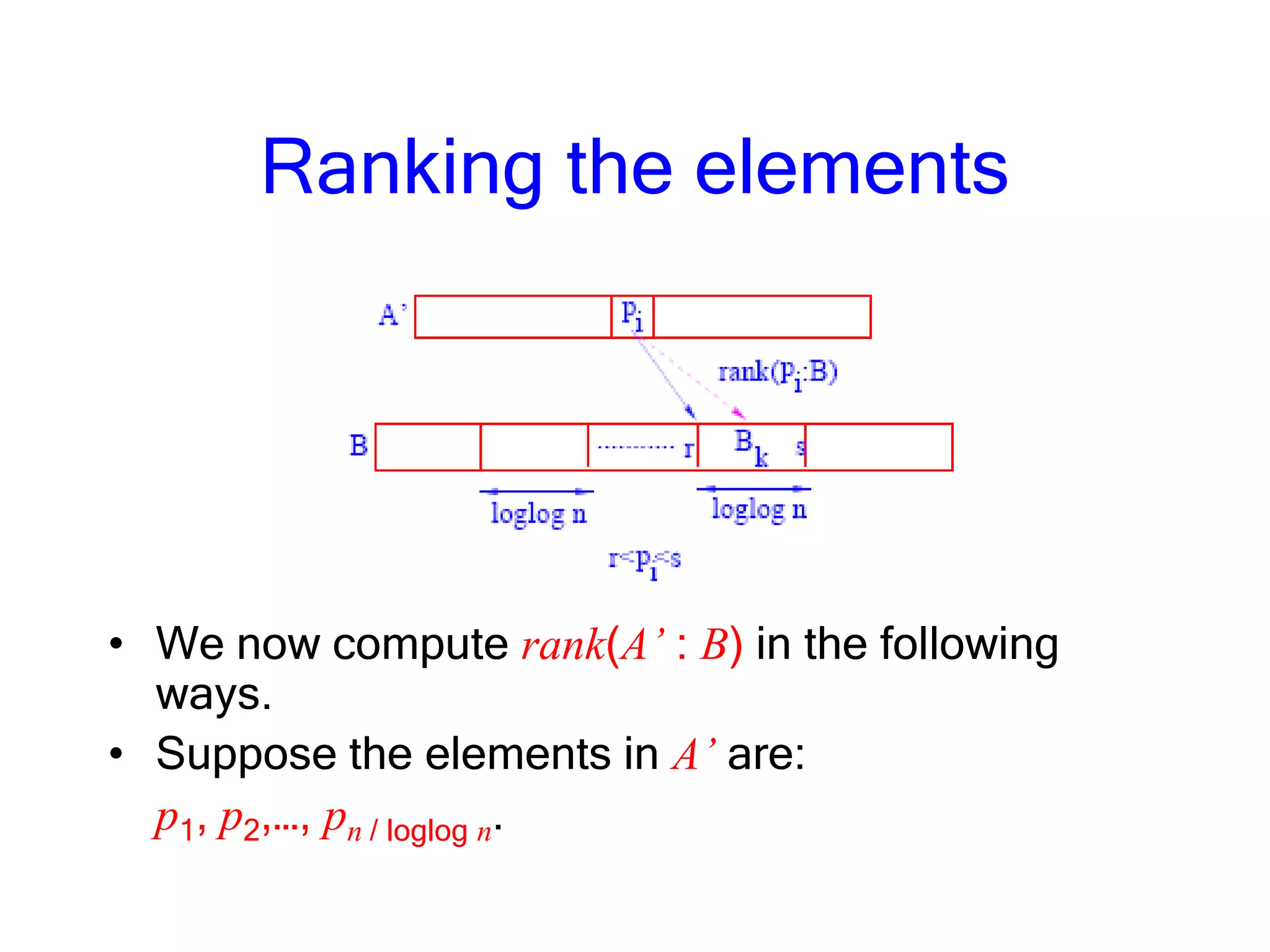
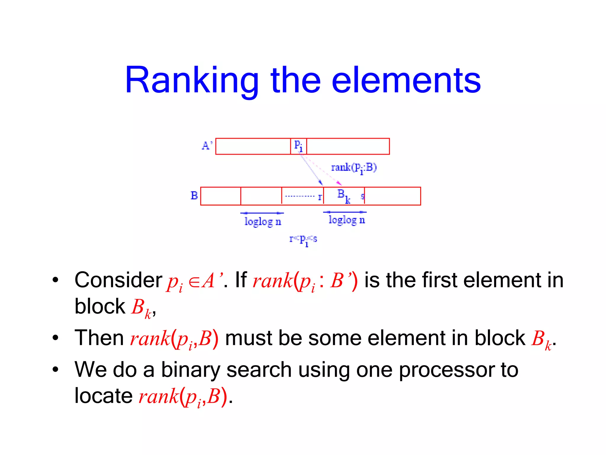
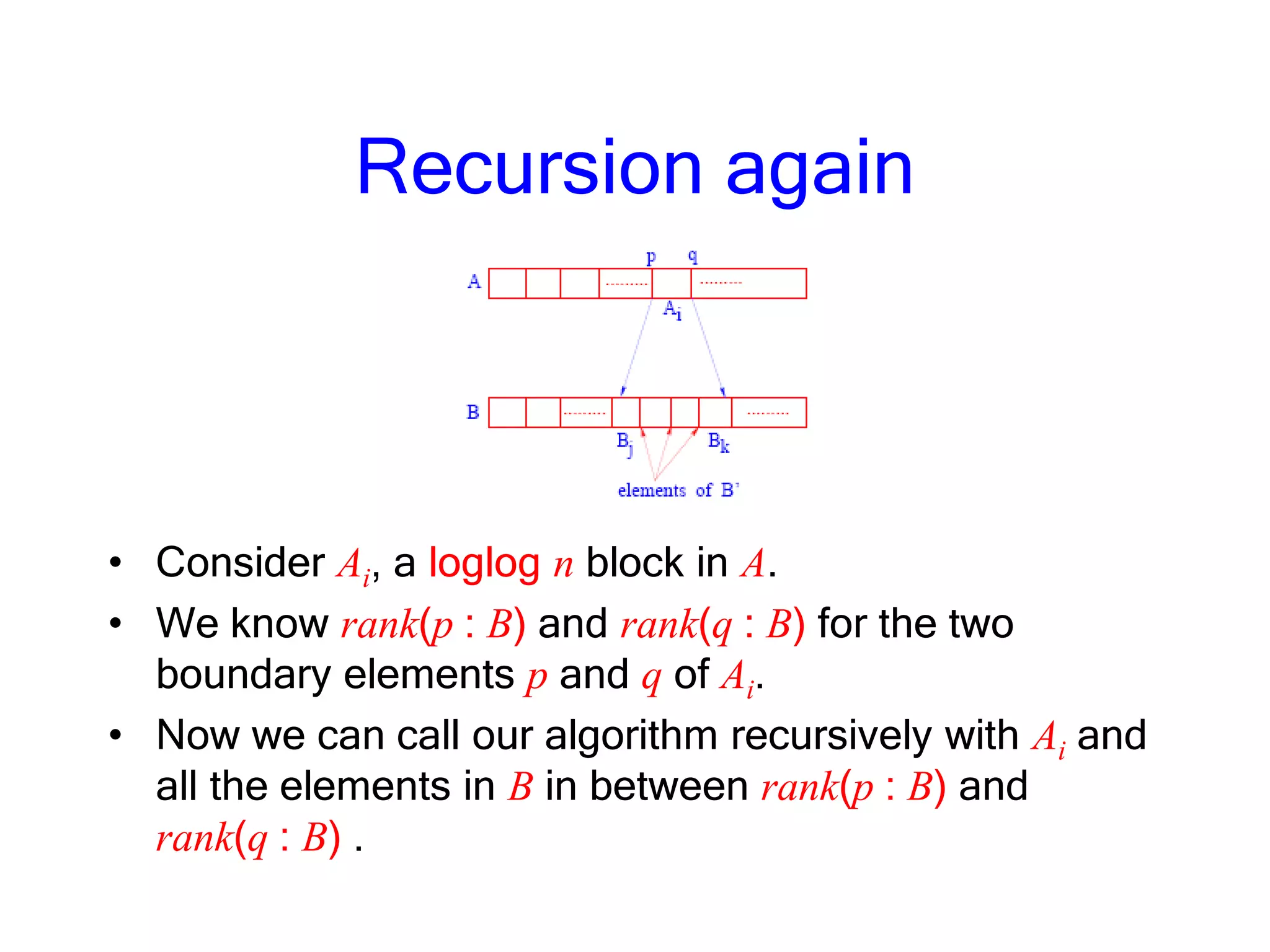
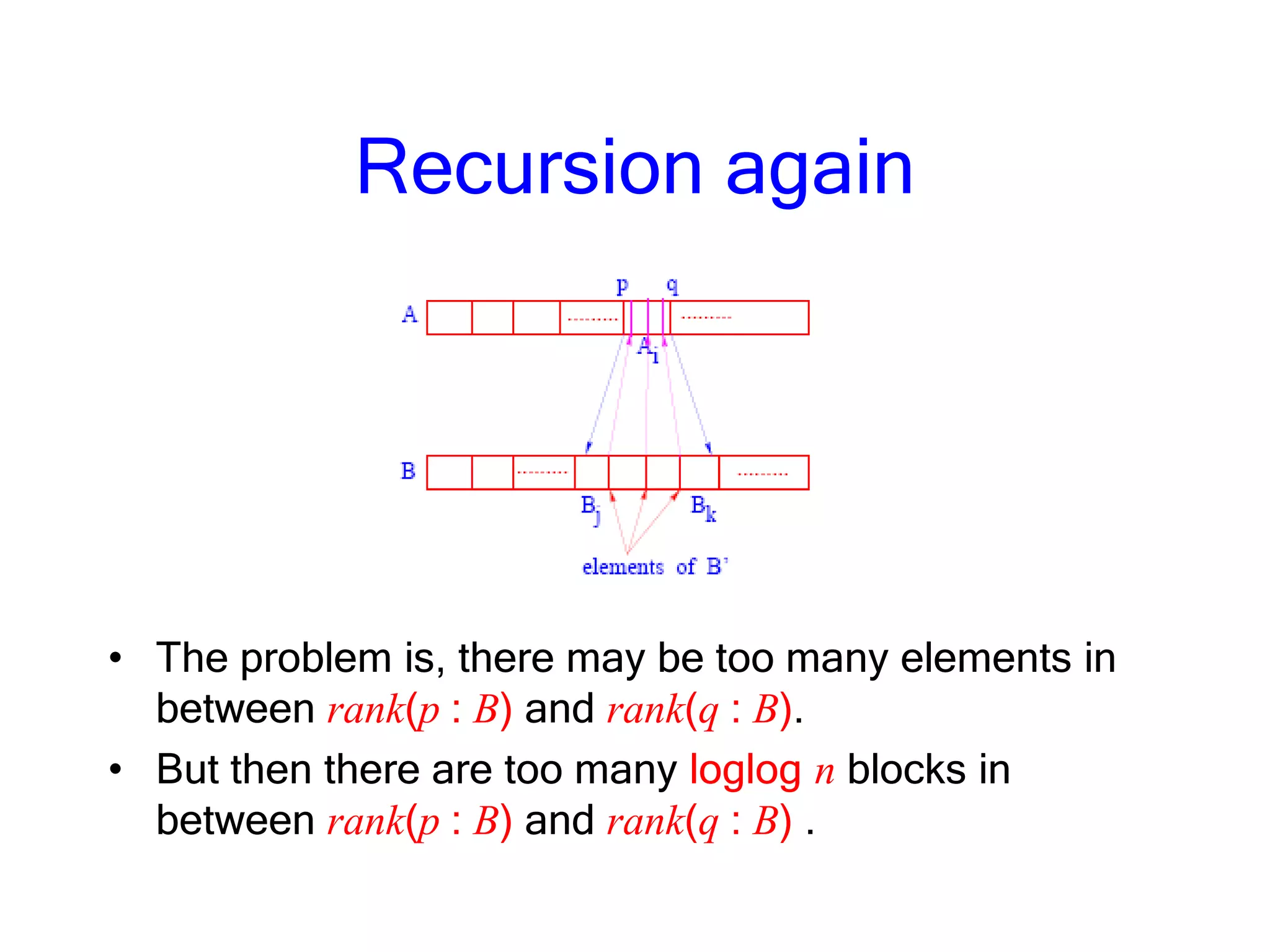
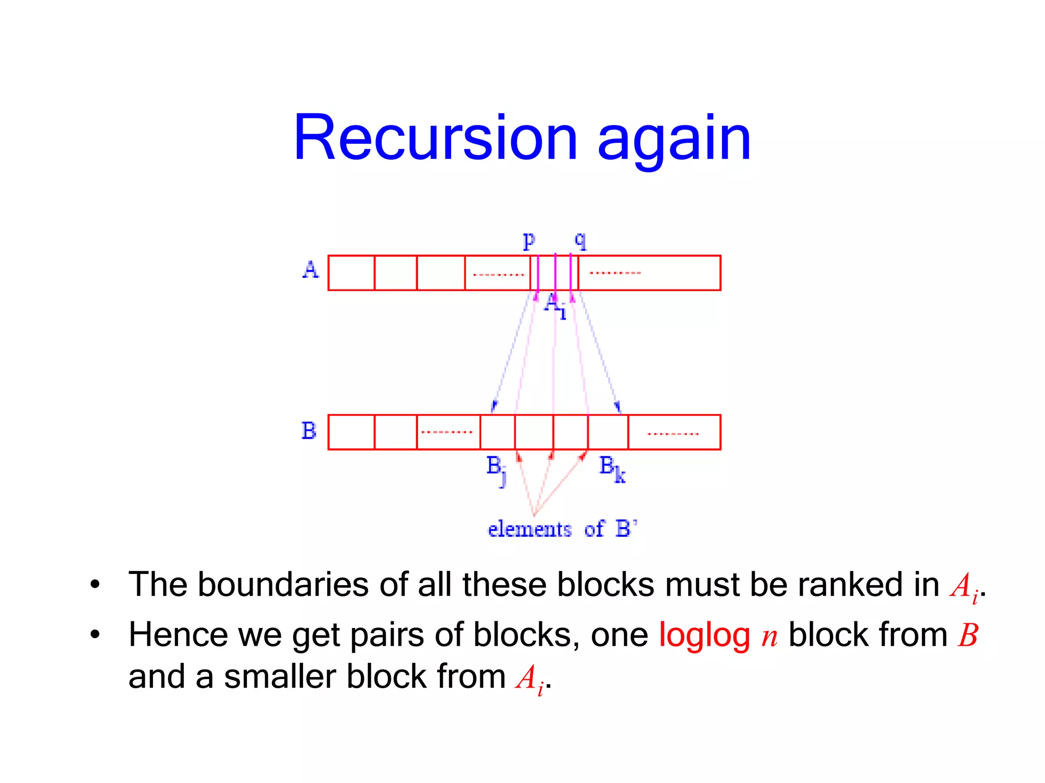
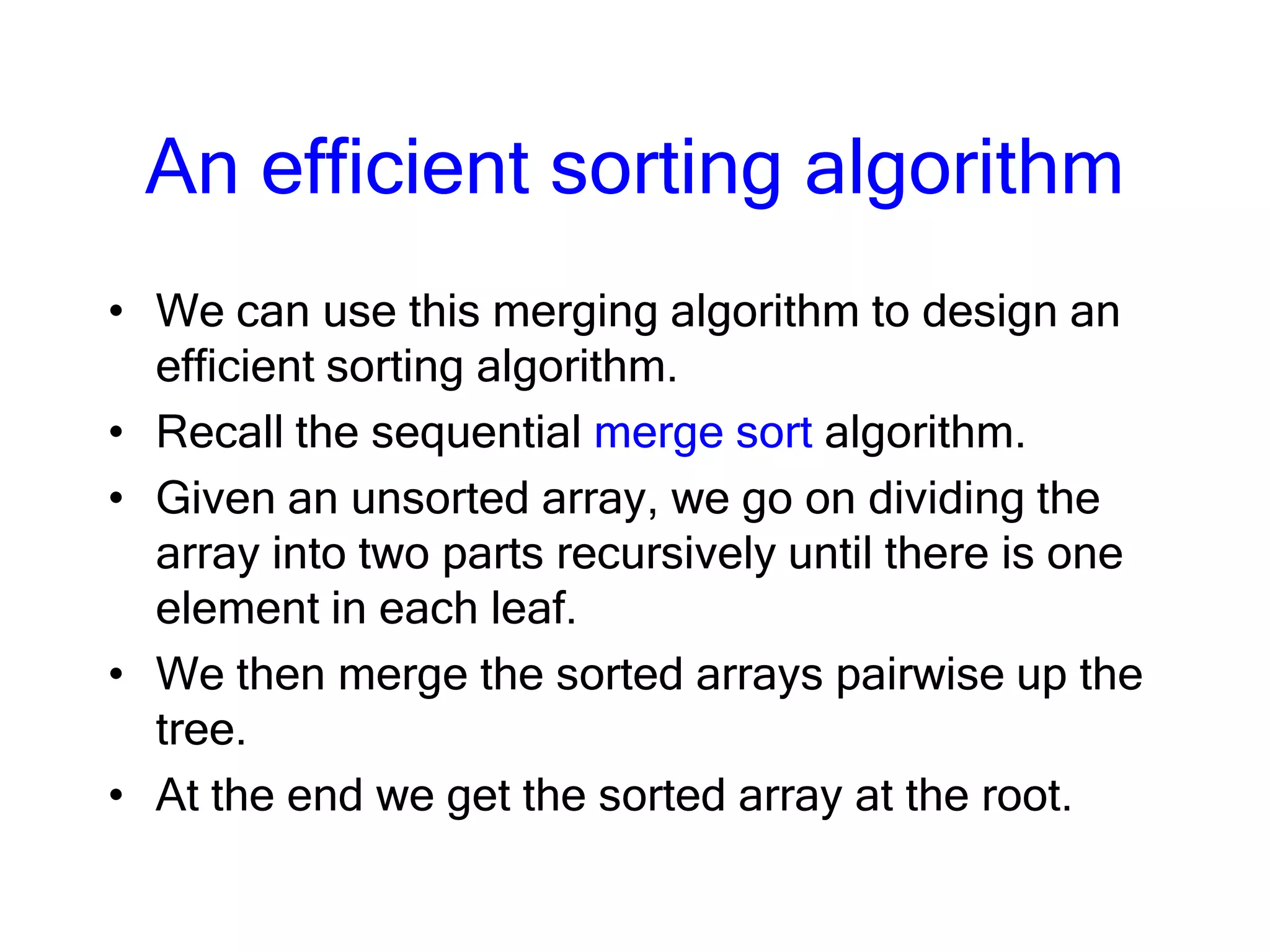
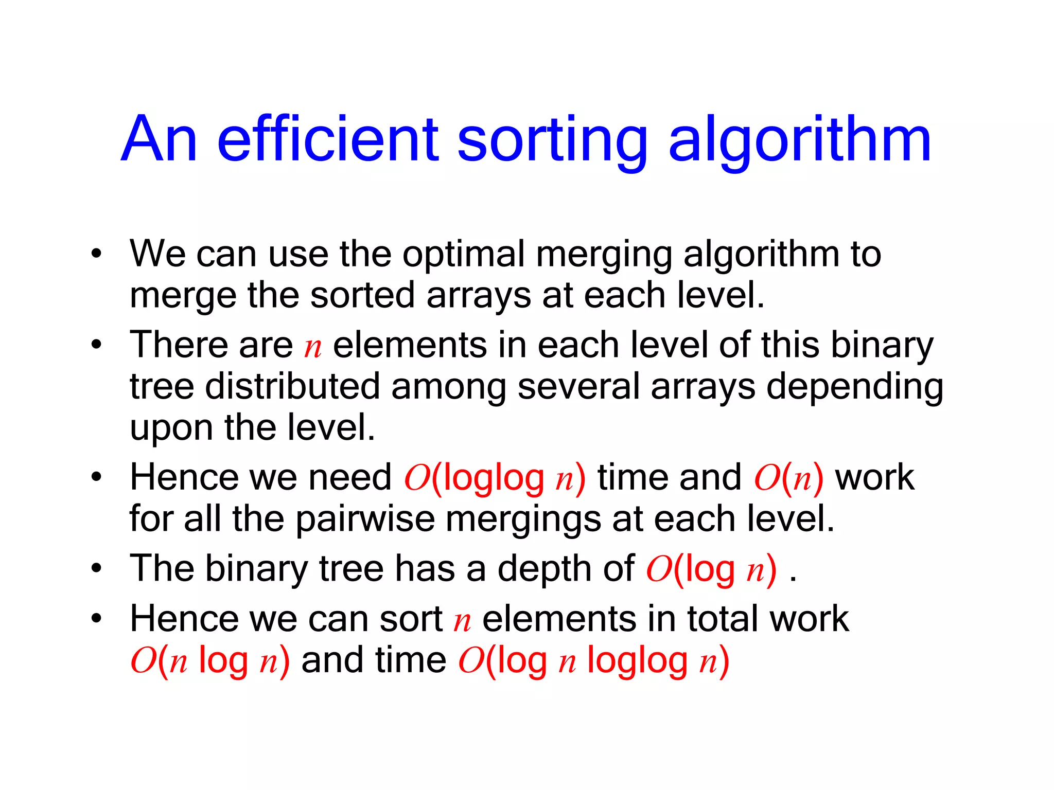
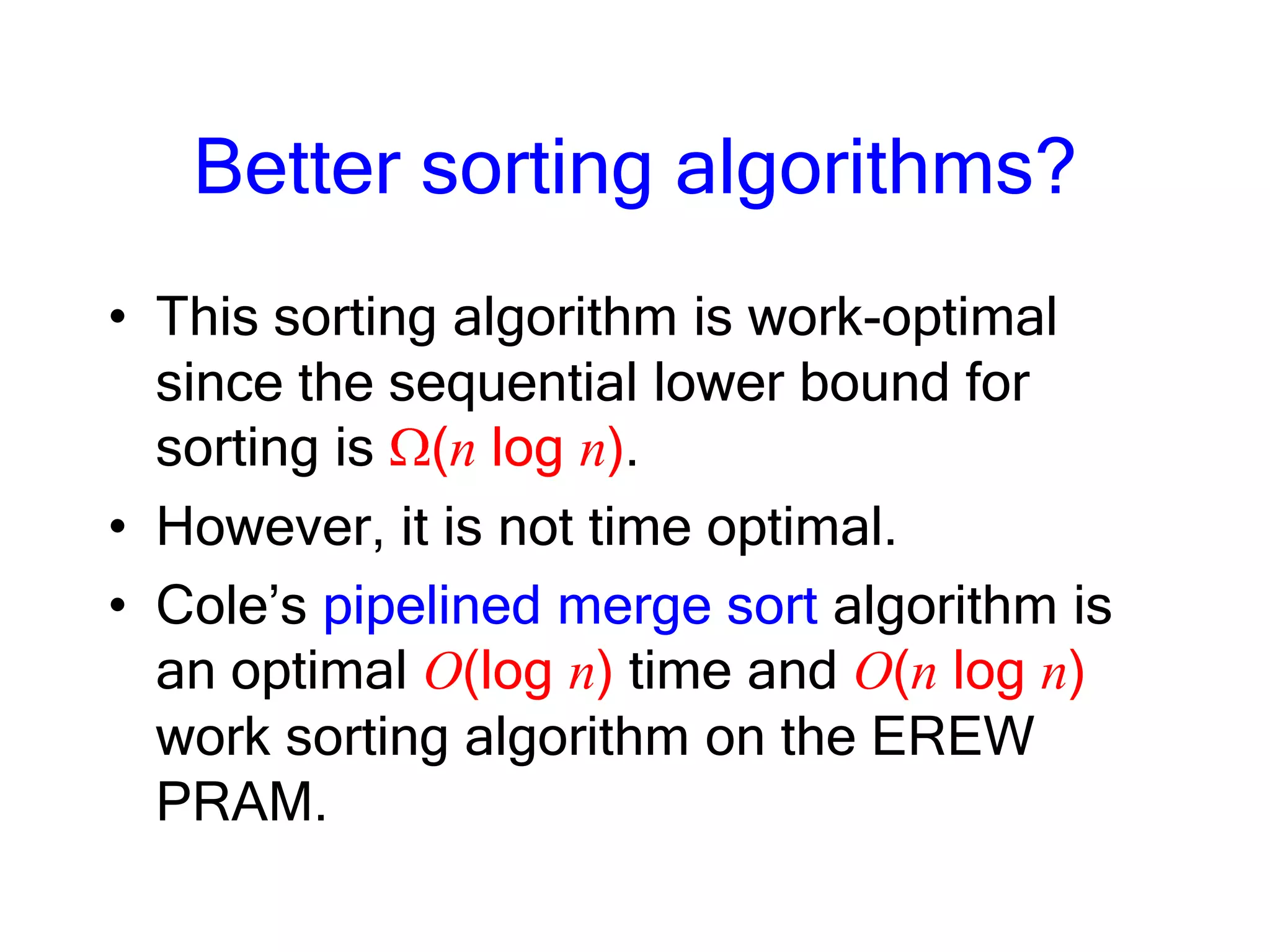
- A parallel search algorithm finds two elements in a sorted array that bracket a query element in logarithmic time using p processors (paragraph 1). - A parallel merging algorithm uses the parallel search to rank and merge two sorted arrays in optimal O(log log n) time and O(n log log n) work (paragraph 2). - An efficient sorting algorithm uses the optimal parallel merging algorithm in a merge sort approach to sort n elements in O(n log n) work and O(log n log log n) time (paragraph 3).

1. An overview of lecture
• A parallel search algorithm
• A parallel merging algorithm
• A parallel sorting algorithm

2. A parallel search algorithm
• We discuss an algorithm for parallel
searching in a sorted array.
• n is the number of elements in a sorted
array S and we use p, p < n processors for
searching.
• The complexity of the parallel searching
algorithm is: .
log( 1)
log( 1)
n
O
p

3. A parallel search algorithm
Input:
(i) A sorted array S = x1,x2,…,xn with n
elements.
(ii) A query element y.
Output: Two elements xi, xi +1 in S such that
xi y xi +1.

4. A parallel search algorithm
• The algorithm consists of a series of iterations to
reduce the size of the array where the element y
is located.
• In each iteration, we divide the current array in
p + 1 equal parts and locate y in one of the parts.
• This is continued until the size of the array where
y is located is reduced to p.
• We then do a direct comparison to find two
elements xi, xi +1 such that xi y xi +1.

5. A parallel search algorithm

6. A parallel search algorithm
• For each of the p + 1 parts of the array, a
processor checks whether y < xl, where xl is the
last element of the part.
• If y < xl, the subarray to the right of xl can be
rejected. If y > xl, the subarray to the left of xl can
be rejected.
• In each iteration we identify only one subarray for
further search.

7. A parallel search algorithm
• When the size of the remaining array is the same
as the number of processors, we do the following.
• We allocate one processor for each element.
• The processor assigned to element xi checks
whether xi y xi +1.
• Hence it takes O(1) time to locate y once the size
of the array has been reduced to p.

8. Complexity
• We need to analyze what is the complexity of
reducing the size of the array to p.
• At the first iteration, we are reducing the size of
the array from n to n/p.
• Suppose, the size reduces to p after k iterations.
• Hence, , which implies n = pk +1.
• . We need the CREW PRAM model.
log
( )
log
n
k O
p
k
n
p
p

9. Merging
• We use the parallel search algorithm to design an
optimal O(loglog n) time merging algorithm.
• rank(x : X) is the number of elements of X that are
x.
• Ranking a sequence Y = (y1, y2, …, yn) in X is the
same as:
• Computing the integer array : (r1, r2, …, rm) where
ri = rank(yi, X).

10. Merging
• If rank(ai, A) = r1 and rank(ai, B) = r2
• rank(ai, A +B) = r1 + r2.
• Hence, ai should go to the entry number r1 + r2 in
the merged array.

11. Ranking a short sequence in a
sorted sequence
• X is a sorted sequence with n elements.
• Y is an arbitrary sorted sequence of size m such
that m = O(ns), where s is a constant and 0 < s < 1.
• If we use processors,
• Then we can rank each element of Y in X
in time.log
( ) (1)
log
n
O O
p
1
( )sn
p O n
m

12. A fast merging algorithm
• We now discuss a fast algorithm for merging two
sorted arrays A and B with n and m elements
each.
• Fast merging is an essential component in any
sorting algorithm based on divide-and-conquer.
• We will first design an O(loglog m) time and
O((m + n) loglog m) work algorithm.
• Then we will improve the work to O(m + n) which
is optimal.

13. A fast merging algorithm
Input: Two sorted sequences A and B of lengths
n and m respectively.
Output: rank(B : A) and rank(A : B).
•We use a strategy similar to the merging
algorithm we discussed earlier.
•We divide the array B into parts, each part
with elements.
•We start with ranking the last element from
each part of B into A.
m
m

14. Ranking a sample of elements
• We start with a sample of elements from B.
• We choose every –th element from B.
• These elements can be ranked in A in O(1)
time through binary search in parallel using m
processors.
m
m
m

15. A parallel search algorithm

16. Ranking elements in O(1) time
m m
m
m m m
m elements
m elements A
B
For every element in B, we allocate processors.m
In one step, we identify the block of elements in
A where an element of B will be ranked.
m
We find the rank in another step.

17. Ranking a sample of elements
• B is partitioned into blocks, each of size .
• After the ranking of the elements from B in A.
• A is also partitioned into blocks.
• We can now merge the blocks in A and B
pairwise recursively.
m m
m
m

18. Independent subproblems
• Consider the first element of B2 and the first element of B3,
the elements r and s.
• Now, r is ranked at u and s is ranked at v.
• Consider an element p such that r < p < s. p must be ranked
in between u and v.
• Hence, all the elements in B2 must be ranked in A2 and vice
verse.

19. Ranking a sample of elements
• Suppose at the current level of recursion, the size
of the two subproblems B’ and A’ are m’ and n’.
• If m’ > n’, then we divide B’ into parts and apply
the algorithm recursively.
• If n’ > m’, we divide A’ into parts and apply the
algorithm recursively.
'm
'n

20. An example

21. Recursion

22. Recursion
• The recursion between all pairs of blocks can
be solved in parallel.
• The recursion stops when the size of the
subproblems is small and we can merge the
very small blocks through a sequential
algorithm in O(1) time.
• At the end of the algorithm, we know rank(B :
A) and rank(A : B). Hence, we can move the
elements to another array in sorted order.

23. Complexity
• The recursion satisfies the recurrences
either :
or,
• The processor requirement is O(m + n).
• The total work done is O(m + n) loglog m.
( ) ( ) (1)T n T n O
( ) ( ) (1)T m T m O

24. An optimal merging algorithm
• The make the algorithm optimal, we need to reduce
the work to O(m + n).
• We use a different sampling strategy and use the fast
algorithm that we have designed. For simplicity, we
assume that each array has n elements.
• We divide the arrays A and B into blocks of size
loglog n.
• We choose the last element from each block as our
sample and form two arrays A’ and B’.
• Hence each of A’ and B’ has elements.loglog
n
n

25. Taking the samples
• Now we compute rank(A’ : B’) and rank(B’ : A’)
using the algorithm we have designed.
• This takes O(loglog n) time and
or O(n) work.
( loglog )
loglog
n
O n
n

26. Ranking the elements
• We now compute rank(A’ : B) in the following
ways.
• Suppose the elements in A’ are:
p1, p2,…, pn / loglog n.

27. Ranking the elements
• Consider pi A’. If rank(pi : B’) is the first element in
block Bk,
• Then rank(pi,B) must be some element in block Bk.
• We do a binary search using one processor to
locate rank(pi,B).

28. Ranking the elements
• We allocate one processor for pi. The processor
does a binary search in Bk.
• Since there are O(loglog n) elements in Bk, this
search takes O(logloglog n) time.
• The search for all the elements in A’ can be done
in parallel and requires processors.
• We can compute rank(B’ : A) in a similar way.
( )
loglog
n
O
n

29. Recursion again
• Consider Ai, a loglog n block in A.
• We know rank(p : B) and rank(q : B) for the two
boundary elements p and q of Ai.
• Now we can call our algorithm recursively with Ai and
all the elements in B in between rank(p : B) and
rank(q : B) .

30. Recursion again
• The problem is, there may be too many elements in
between rank(p : B) and rank(q : B).
• But then there are too many loglog n blocks in
between rank(p : B) and rank(q : B) .

31. Recursion again
• The boundaries of all these blocks must be ranked in Ai.
• Hence we get pairs of blocks, one loglog n block from B
and a smaller block from Ai.

32. Solving the subproblems
• Now each of the two blocks participating in a
subproblem has size at most loglog n.
• And there are such pairs.
• We assign one processor to each pair. This
processor merges the elements in the pair
sequentially in O(loglog n) time.
• All the mergings can be done in parallel since we
have processors.
( )
loglog
n
O
n
loglog
n
n

33. Complexity
• Computing rank(A’ : B’) and rank(B’ : A’) take
O(loglog n) time and O(n) work.
• Computing rank(A’ : B) and rank(B’ : A) take
O(loglog n) time and O(n) work.
• The final merging also takes the same time and
work.
• Hence, we can merge two sorted arrays of length
n each in O(n) work and O(loglog n) time on the
CREW PRAM.

34. An efficient sorting algorithm
• We can use this merging algorithm to design an
efficient sorting algorithm.
• Recall the sequential merge sort algorithm.
• Given an unsorted array, we go on dividing the
array into two parts recursively until there is one
element in each leaf.
• We then merge the sorted arrays pairwise up the
tree.
• At the end we get the sorted array at the root.

35. An efficient sorting algorithm
• We can use the optimal merging algorithm to
merge the sorted arrays at each level.
• There are n elements in each level of this binary
tree distributed among several arrays depending
upon the level.
• Hence we need O(loglog n) time and O(n) work
for all the pairwise mergings at each level.
• The binary tree has a depth of O(log n) .
• Hence we can sort n elements in total work
O(n log n) and time O(log n loglog n)

36. Better sorting algorithms?
• This sorting algorithm is work-optimal
since the sequential lower bound for
sorting is (n log n).
• However, it is not time optimal.
• Cole’s pipelined merge sort algorithm is
an optimal O(log n) time and O(n log n)
work sorting algorithm on the EREW
PRAM.