Downloaded 88 times


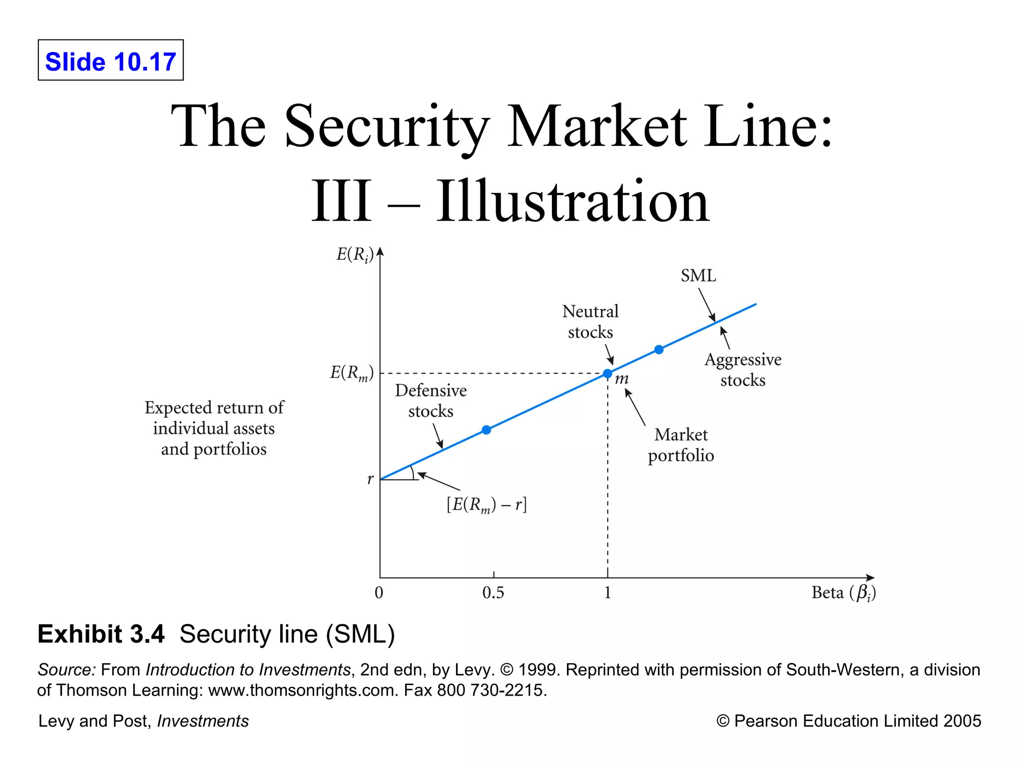
![The Security Market Line: I Under the assumptions of the CAPM, only compensating investors for bearing systemic risk, the following linear risk-return relation (for both individual assets and portfolios) should hold: E ( R i ) r [ E ( R m ) – r ] i Expected Rate of Return Risk-Free Rate Risk Premium](https://image.slidesharecdn.com/lpch10-091226092059-phpapp02/75/L-Pch10-14-2048.jpg)
![The Security Market Line: II – The Risk Premium The risk premium is the expected return investors require above and beyond what can be earned on the risk-free asset: [ E ( R m ) – r ] i market risk premium Asset i’s Beta](https://image.slidesharecdn.com/lpch10-091226092059-phpapp02/75/L-Pch10-16-2048.jpg)
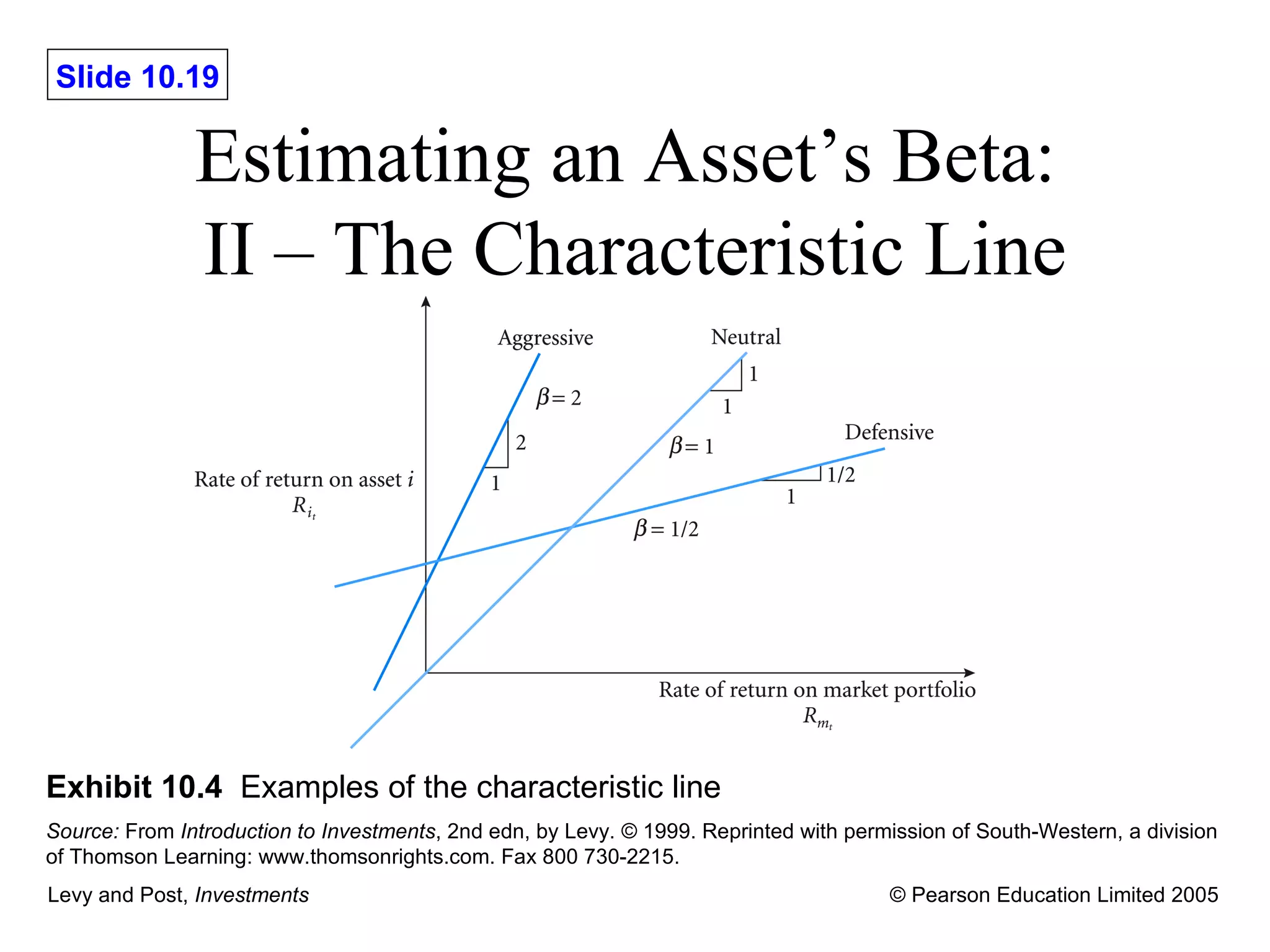
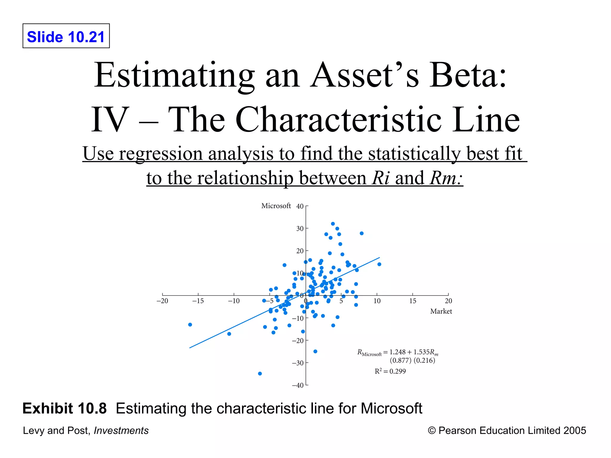
![Estimating an Asset ’s Beta: III – The Characteristic Line The Characteristic Line can be written as: R i – r i i R m – r ] e i i intercept of the regression line i slope of the regression line e t firm-specific factor with mean E ( e i )=0 and variance 2 e,i](https://image.slidesharecdn.com/lpch10-091226092059-phpapp02/75/L-Pch10-20-2048.jpg)

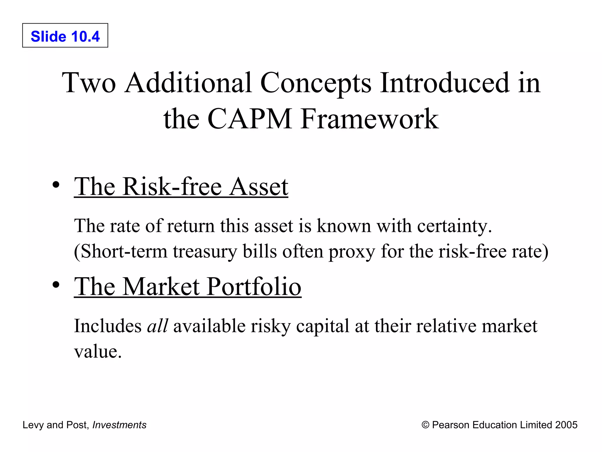
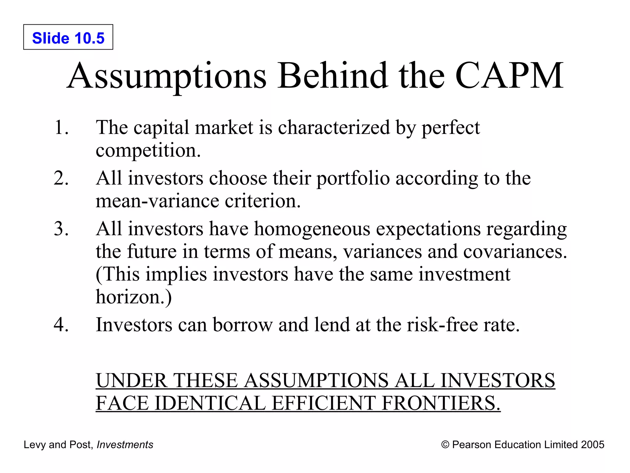
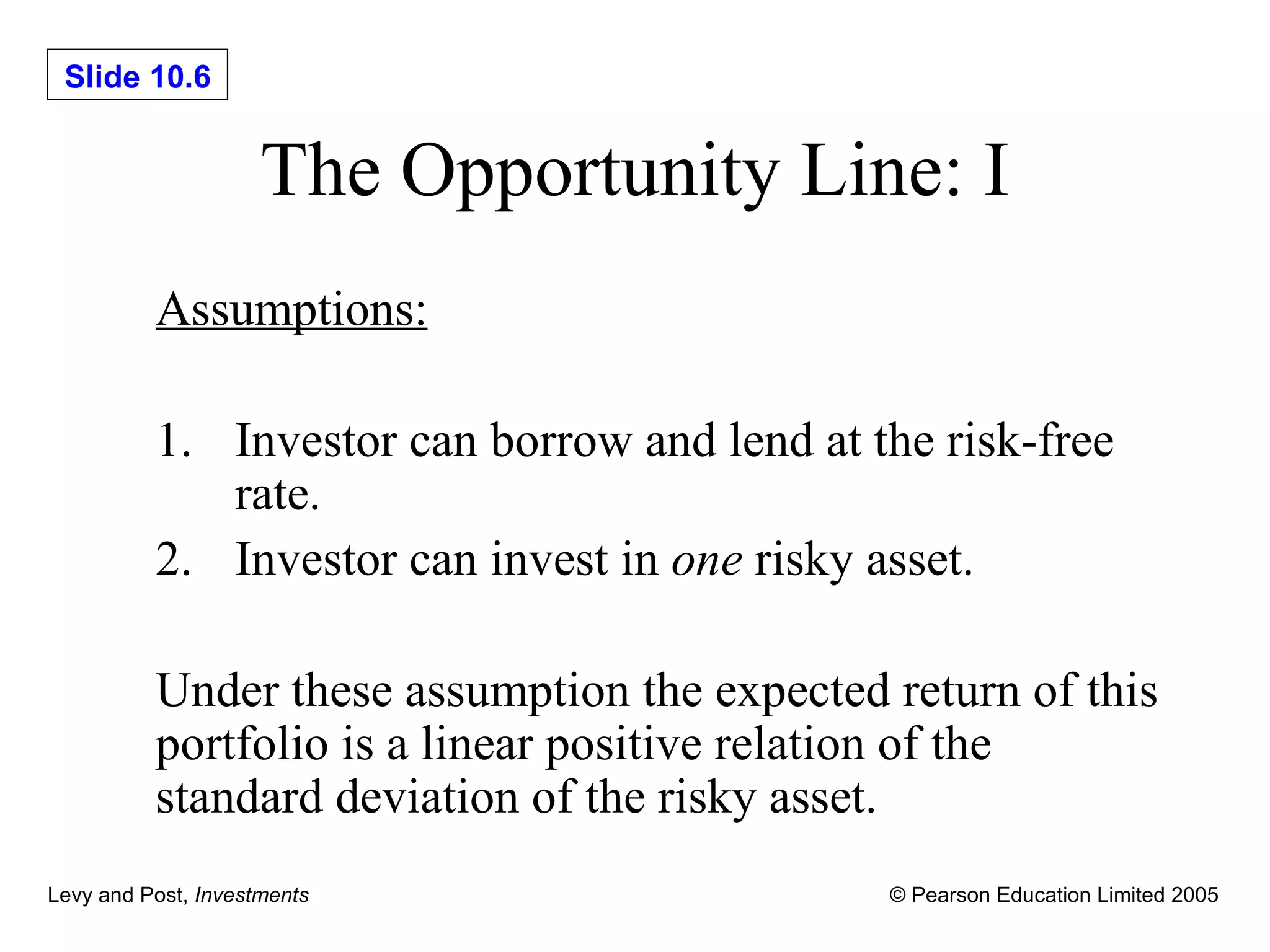
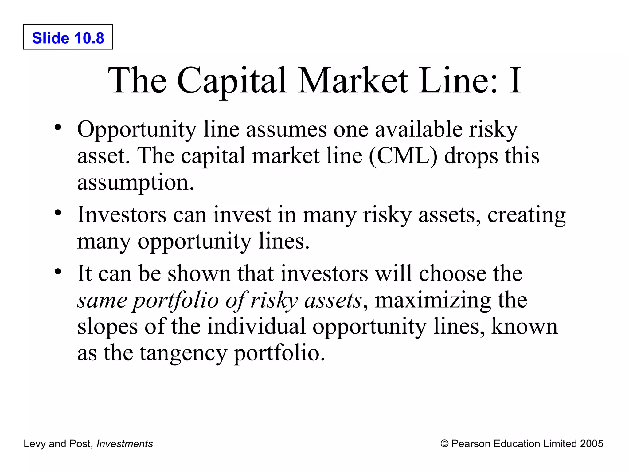
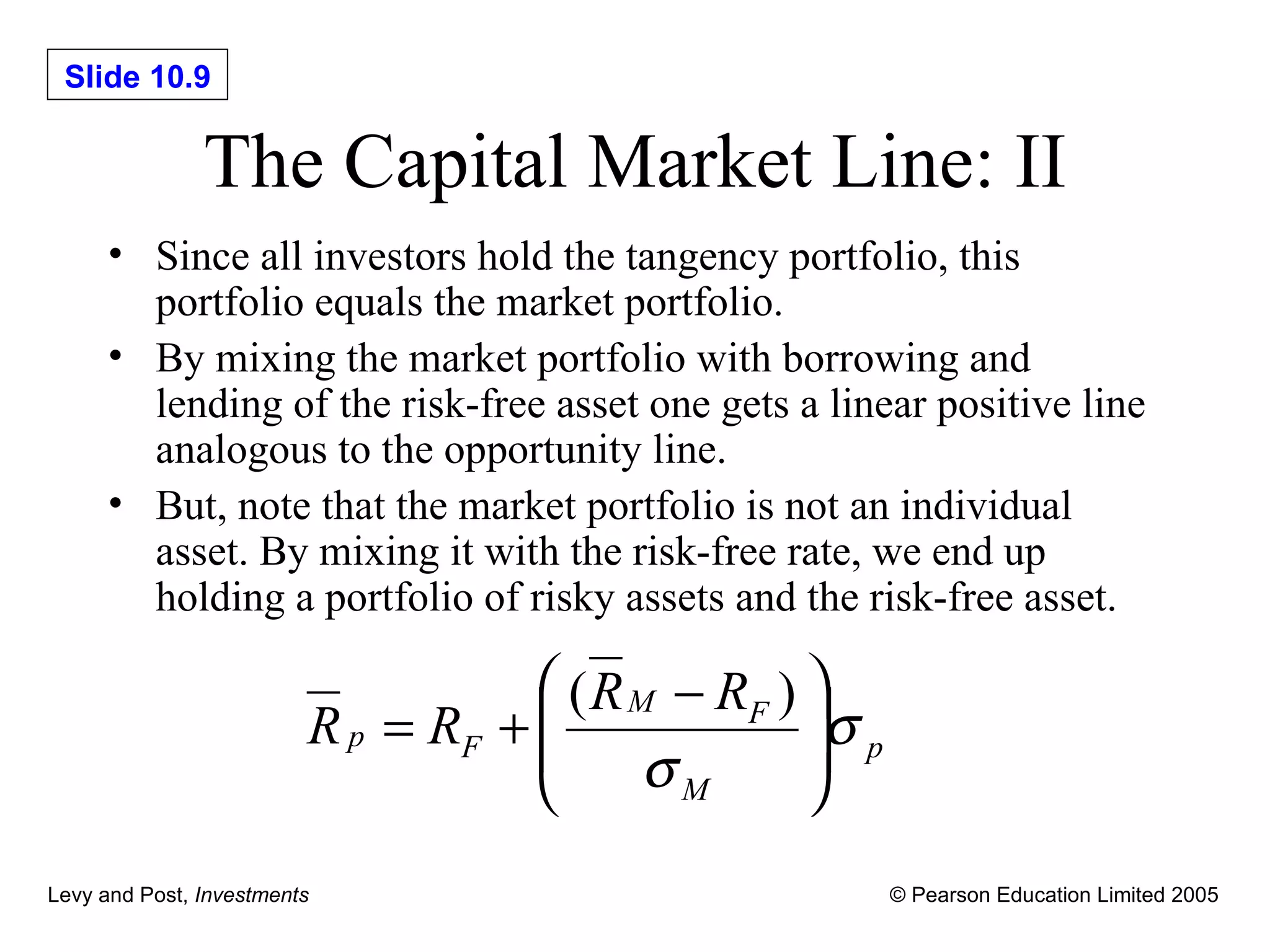
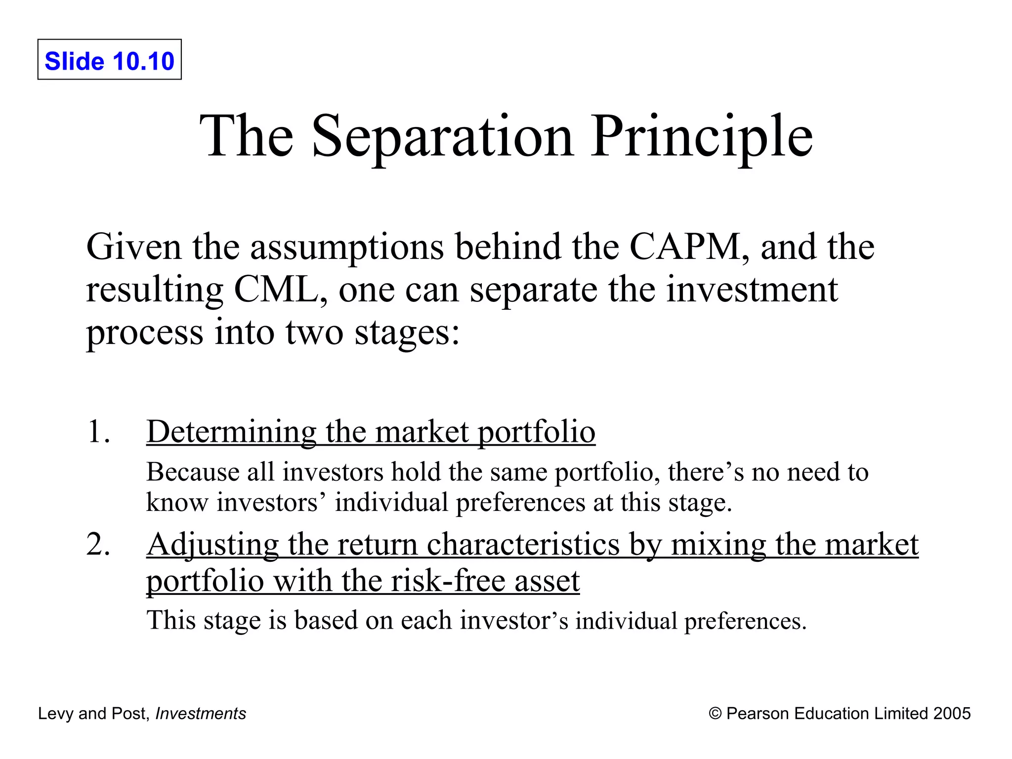
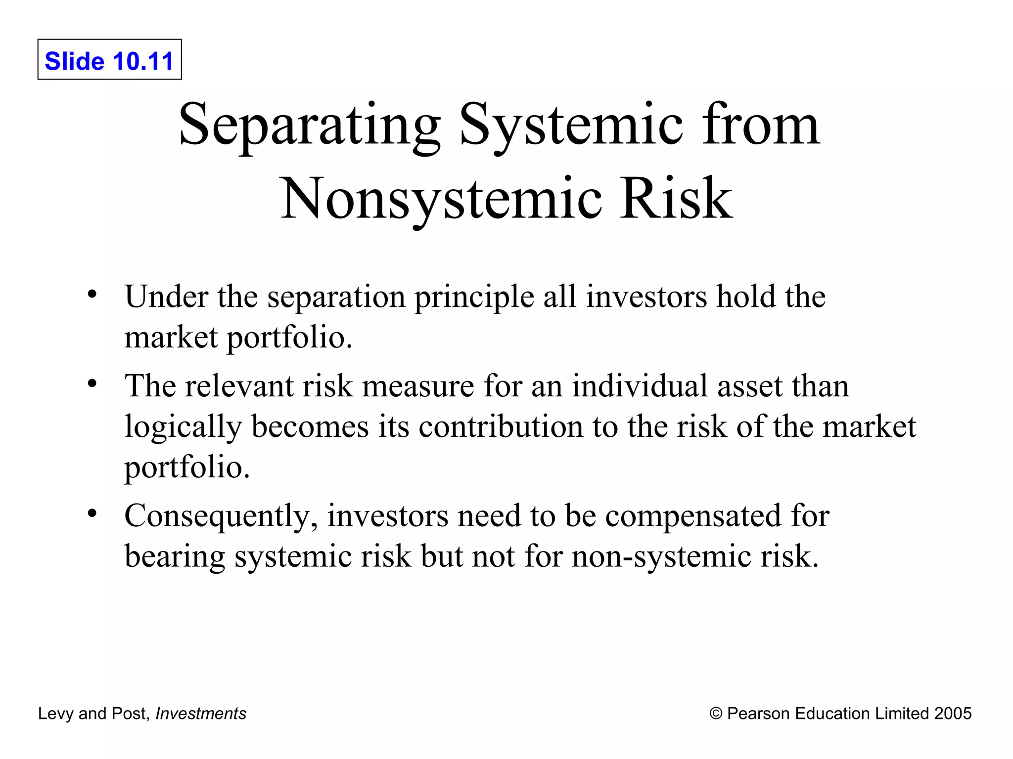
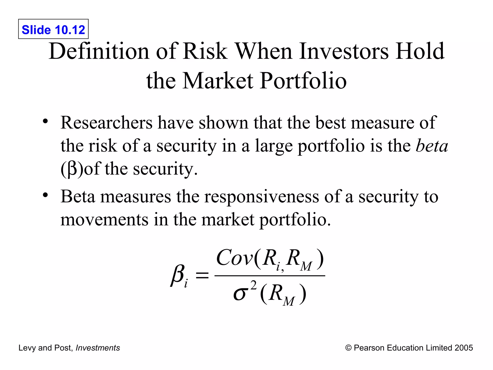
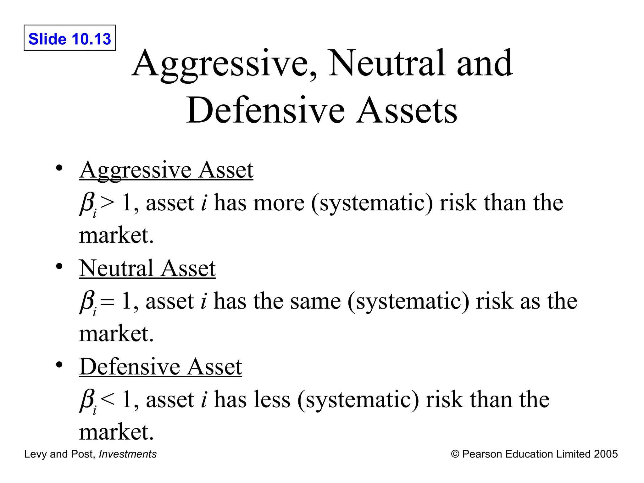
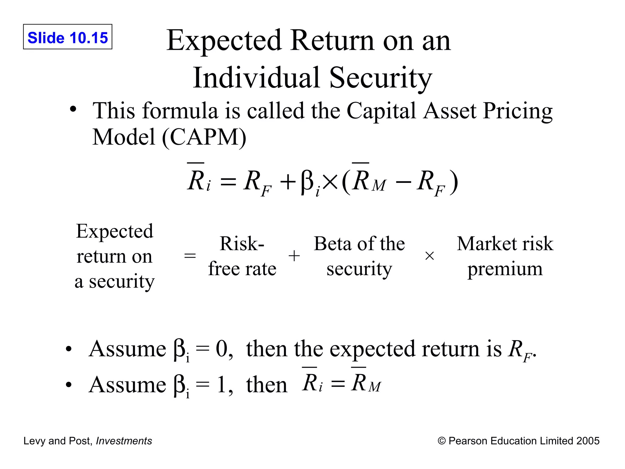
The document provides an overview of the Capital Asset Pricing Model (CAPM). It defines key concepts such as systematic and non-systematic risk, the security market line, and beta. It also discusses how beta is estimated using regression analysis and the characteristic line. Empirical tests are often used to evaluate whether asset prices conform to the predictions of the CAPM.


