Capital Asset Pricing Model
(CAPM)
Assumptions of CAPM
1. All investors aim to maximize economic utilities.
2. All investors make decision based on the return and standard deviation.
3. All investors have Homogenous expectation towards input factors that is used to make
portfolio.
4. All investors can lend and borrow unlimited amount under the risk free rate of return.
5. Short selling is allowed.
6. Securities as highly divisible.
7. All securities are liquid, can be sold at current market price.
8. No transaction fee.
Assumptions of CAPM
9. There is no inflation in the market.
10.There is no tax payable for investors.
11. All investors are price-takers
12. The capital market is in equilibrium.
Capital Market Equilibrium
Occurs when there is no more incentive for investors to trade.
Assumptions under capital market equilibrium:
1. All investors will choose market portfolio.
2. Market portfolio contained optimized securities, efficient frontier.
Market Portfolio
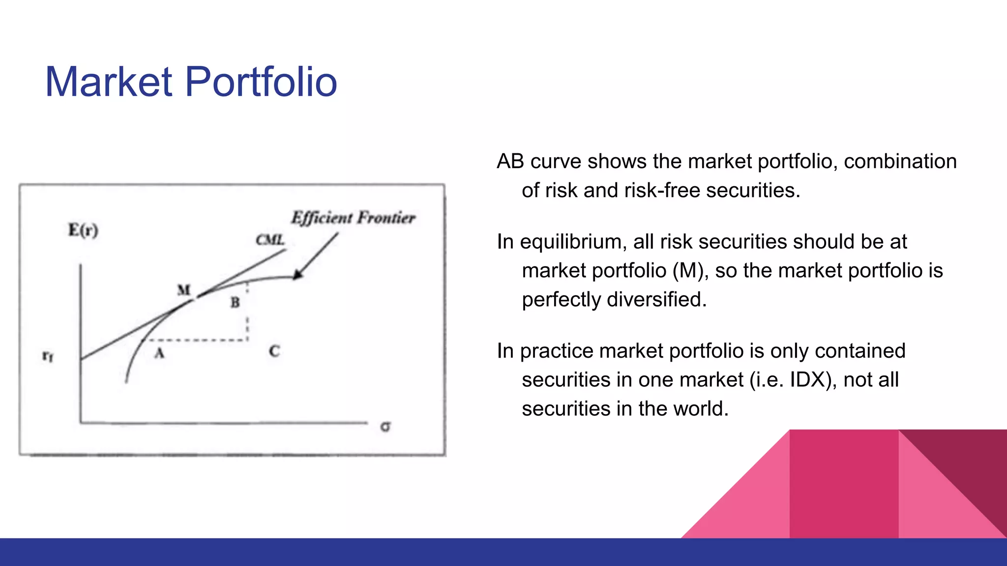
AB curve shows the market portfolio, combination
of risk and risk-free securities.
In equilibrium, all risk securities should be at
market portfolio (M), so the market portfolio is
perfectly diversified.
In practice market portfolio is only contained
securities in one market (i.e. IDX), not all
securities in the world.
Capital Market Line
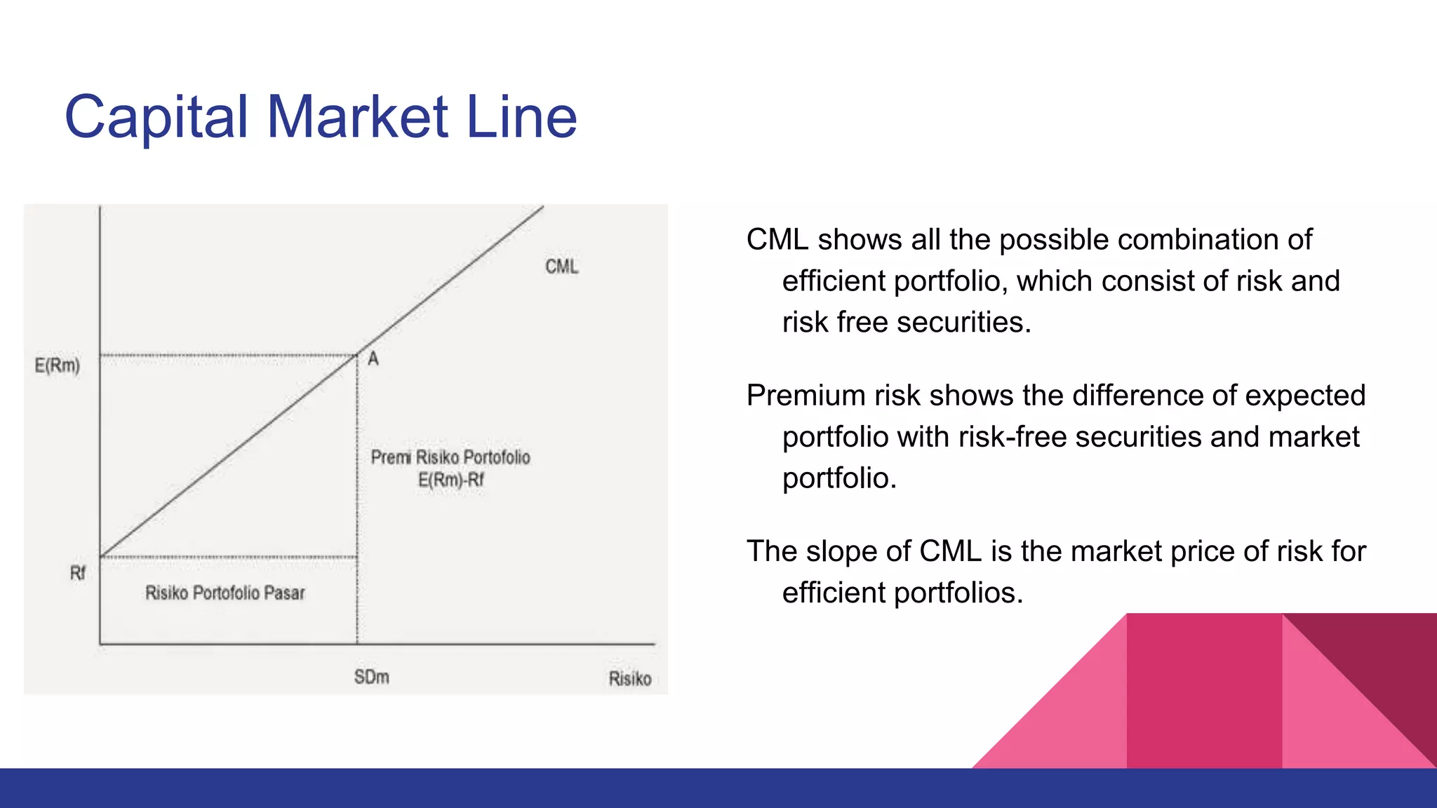
CML shows all the possible combination of
efficient portfolio, which consist of risk and
risk free securities.
Premium risk shows the difference of expected
portfolio with risk-free securities and market
portfolio.
The slope of CML is the market price of risk for
efficient portfolios.
Capital Market Line
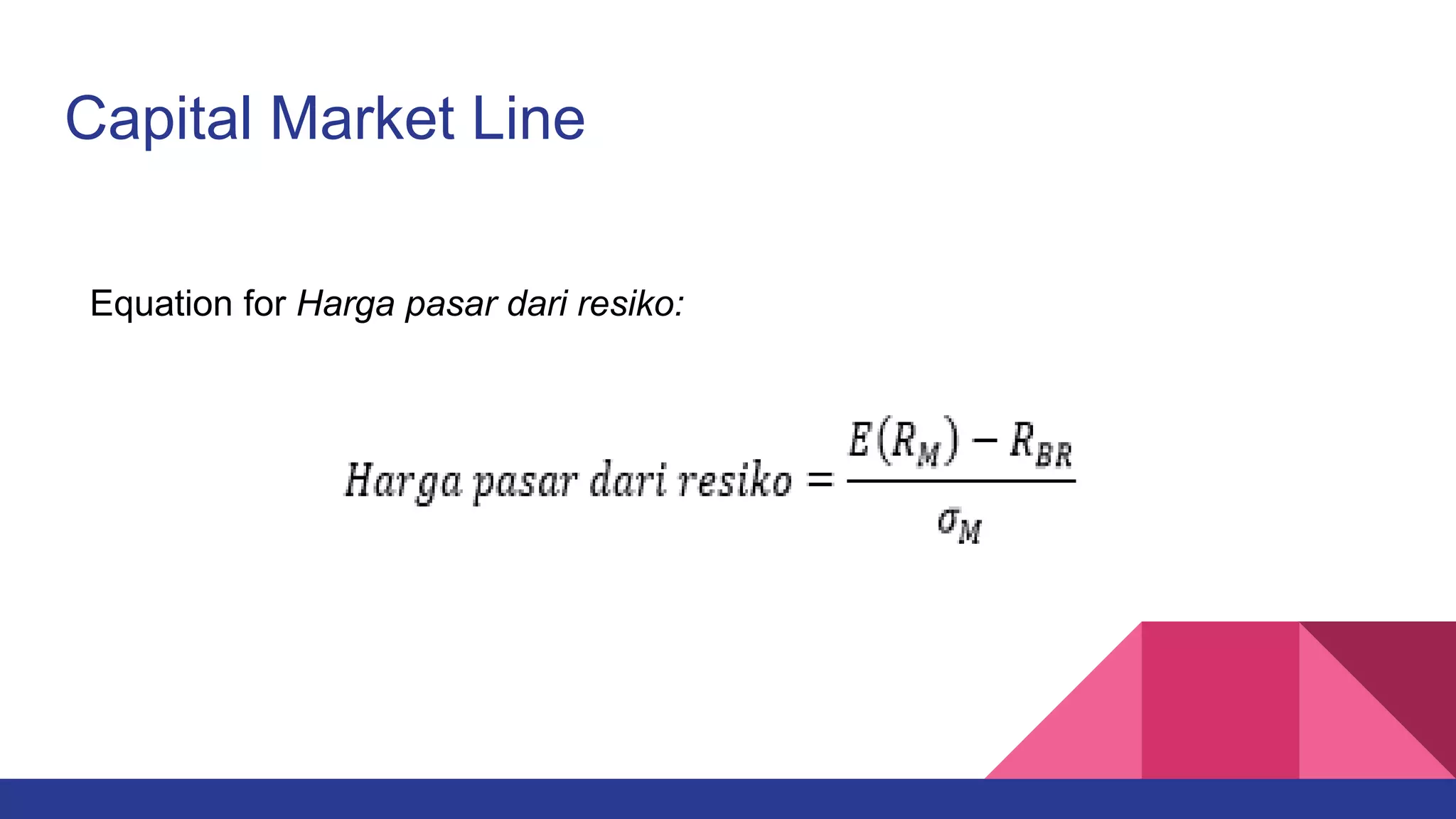
Equation for Harga pasar dari resiko:
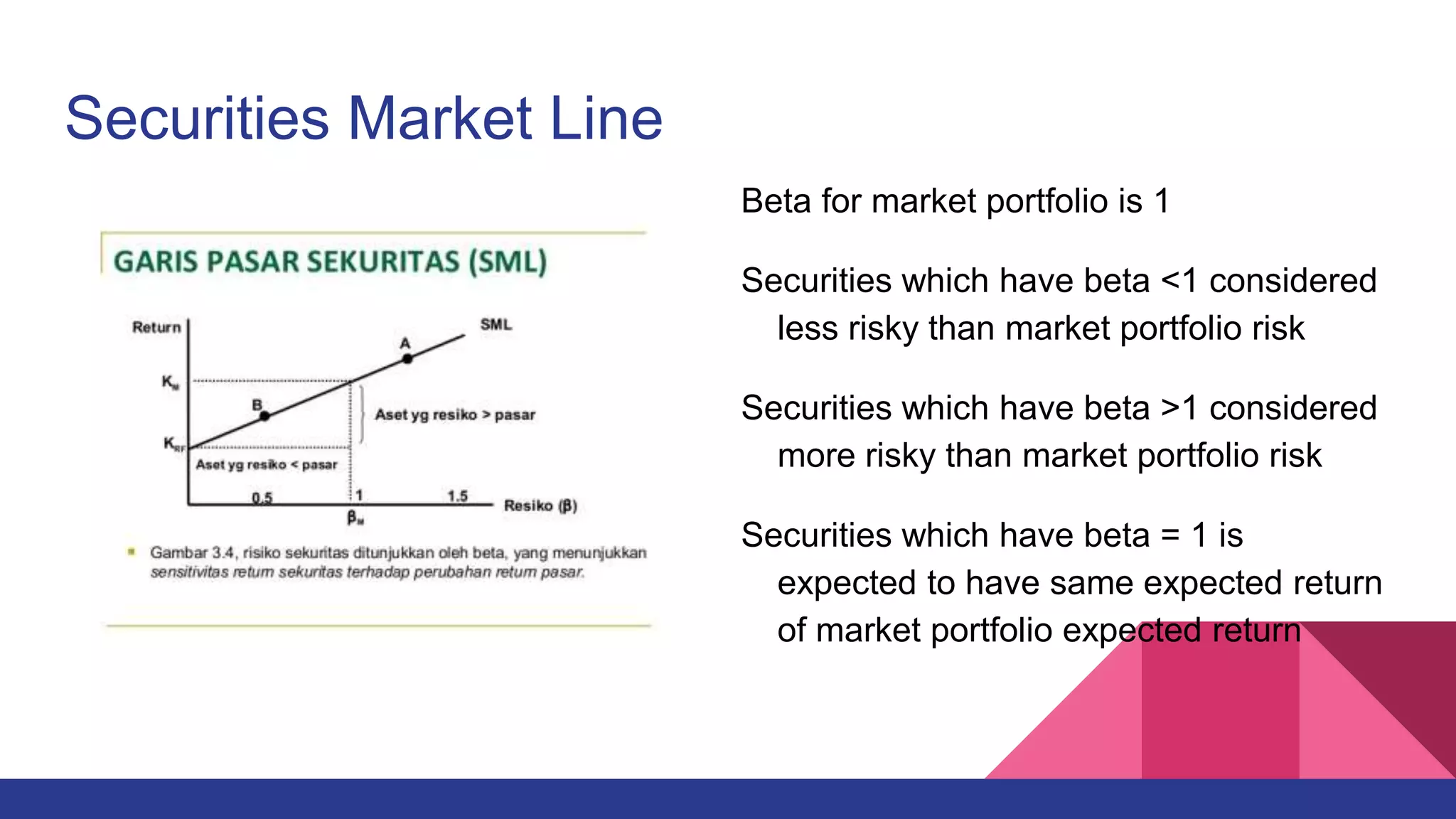
Securities Market Line
Depict tradeoff between risk and expected return for efficient portfolio, but not for individual securities
In portfolio, additional expected return happens because of additional risk from portfolio itself
In individual securities, additional expected return is because of additional individual securities risk
which is determined by Beta
Beta determined the amount of additional expected return for individual securities with argument that
for portfolio which is perfectly diversified, non systematic risk is gone
This argument is based on the assumption homogenous expectation (every investor will create
perfectly diversified portfolio. leaving only Beta risk)
Securities Market Line
Beta for market portfolio is 1
Securities which have beta <1 considered
less risky than market portfolio risk
Securities which have beta >1 considered
more risky than market portfolio risk
Securities which have beta = 1 is
expected to have same expected return
of market portfolio expected return
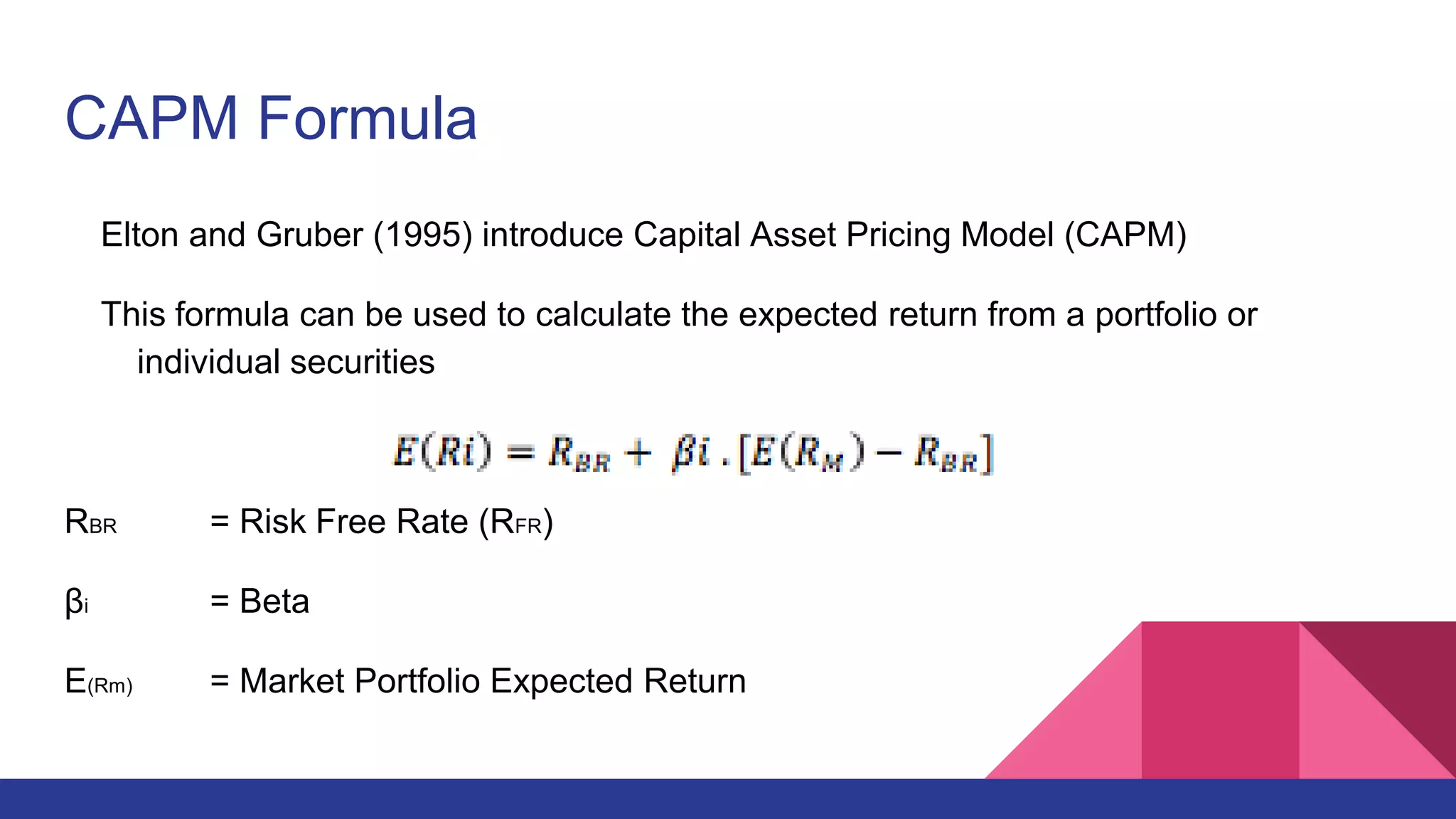
CAPM Formula
Elton and Gruber (1995) introduce Capital Asset Pricing Model (CAPM)
This formula can be used to calculate the expected return from a portfolio or
individual securities
RBR = Risk Free Rate (RFR)
βi = Beta
E(Rm) = Market Portfolio Expected Return
CAPM Example
RFR = 9%;E(Rm) = 13%; βA = 1,3
E(RA) = 9% + (13% - 9%) . 1,3
= 9% + 5,2%
= 14,2%
To check whether the securities are undervalued or overvalued is by comparing the
expected return with the real return
Example 2
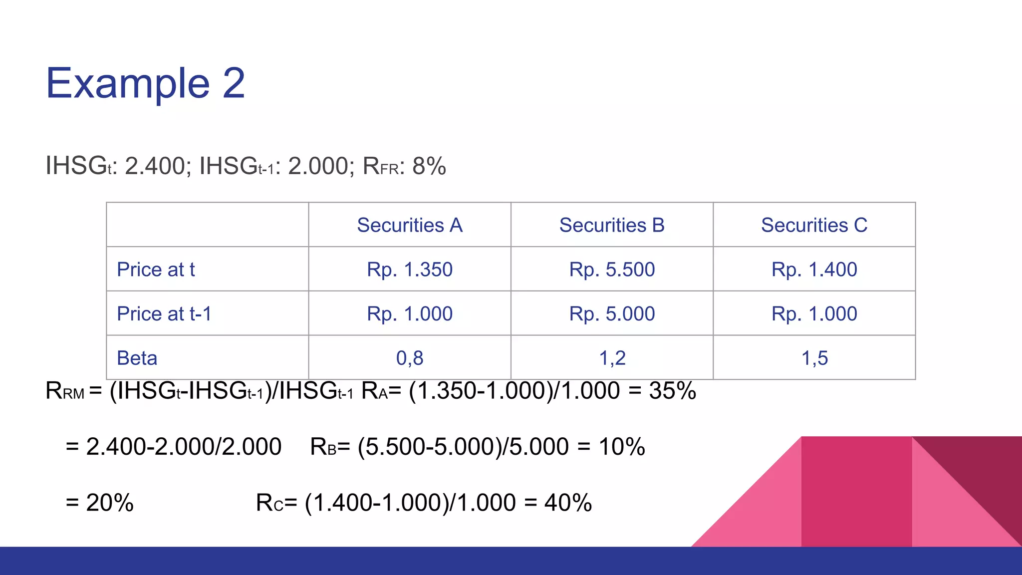
IHSGt: 2.400; IHSGt-1: 2.000; RFR: 8%
RRM = (IHSGt-IHSGt-1)/IHSGt-1 RA= (1.350-1.000)/1.000 = 35%
= 2.400-2.000/2.000 RB= (5.500-5.000)/5.000 = 10%
= 20% RC= (1.400-1.000)/1.000 = 40%
Securities A Securities B Securities C
Price at t Rp. 1.350 Rp. 5.500 Rp. 1.400
Price at t-1 Rp. 1.000 Rp. 5.000 Rp. 1.000
Beta 0,8 1,2 1,5
Example 2(Cont.)
Real Return:
E(RA)= 8% + 0,8 (20%-8%)= 17,6%
E(RB)= 8% + 1,2 (20%-8%)= 22,4%
E(RC)= 8% + 1,5 (20%-8%)= 26,0%
Conclusion:
Securities A= Undervalued; Securities B= Overvalued;
Securities C= Undervalued
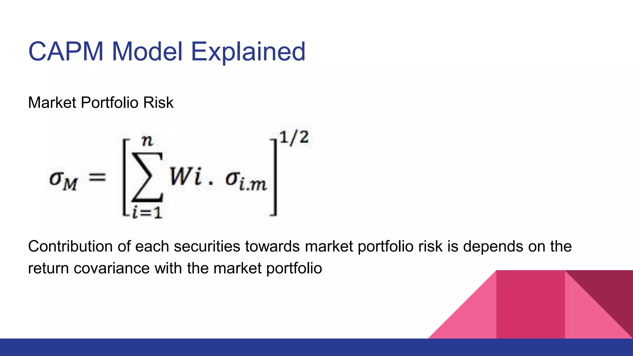
CAPM Model Explained
Market Portfolio Risk
Contribution of each securities towards market portfolio risk is depends on the
return covariance with the market portfolio
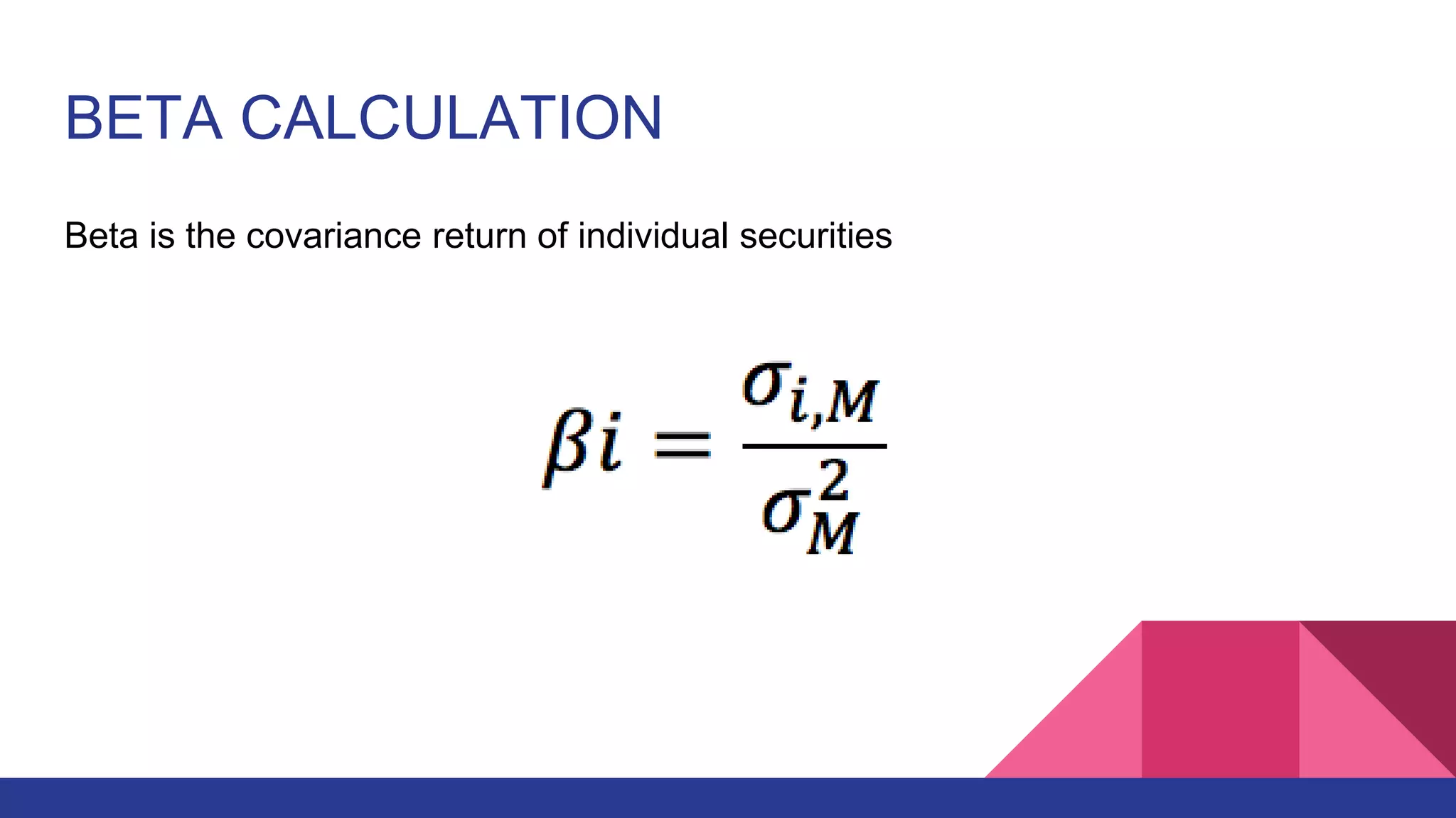
BETA CALCULATION
Beta is the covariance return of individual securities
CAPM Model Explained (cont.)
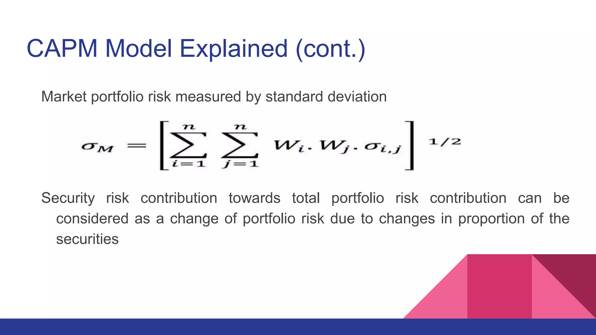
Market portfolio risk measured by standard deviation
Security risk contribution towards total portfolio risk contribution can be
considered as a change of portfolio risk due to changes in proportion of the
securities
Empirical Testing of CAPM
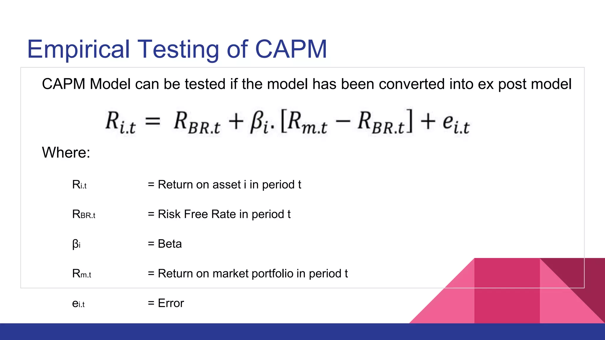
CAPM Model can be tested if the model has been converted into ex post model
Where:
Ri.t = Return on asset i in period t
RBR.t = Risk Free Rate in period t
βi = Beta
Rm.t = Return on market portfolio in period t
ei.t = Error
The difference between Ex ante and Ex post
Ex Ante
Theoretical model
Slope of Securities Market Line (SML) should
be positive
Ex Post
Empirical model
Slope of Securities Market Line (SML) Should
be 0 or negative
E(RM)
E(Ri)
M
RBR
0 1,0
Beta
1,0 Beta
M
RM
0
RBR
Ri
Empirical Testing of CAPM (cont.)
Predictions:
Intercept δ0 is expected not differ significantly to 0
Beta is the only factor that explains return of security risk
.
Relationship between Return and Risk should be Linear
δ1 should be positive or the return on market portfolio must be higher than Risk-free Rate of
Return
Results of testing the CAPM model
The value of intercept is significantly higher than 0
The coefficient of beta has small value than return on market portfolio minus
Risk-free Rate of Return
The coefficient of beta has positive value / δ1 > 0
Other factors (beside Beta) can explain the portion of securities return
P/E ratio (Basu 1977)
Firm-size (Banz 1981 and Reinganum 1981)
Dividend yield (Rosenberg and Marathe 1977, Litzenberger and Ramaswamy,1979)
Seasonality effect or January effect (Keim,1985)
Capital Asset Pricing Model (CAPM)

Capital Asset Pricing Model (CAPM)

  • 1.
  • 2.
    Assumptions of CAPM 1.All investors aim to maximize economic utilities. 2. All investors make decision based on the return and standard deviation. 3. All investors have Homogenous expectation towards input factors that is used to make portfolio. 4. All investors can lend and borrow unlimited amount under the risk free rate of return. 5. Short selling is allowed. 6. Securities as highly divisible. 7. All securities are liquid, can be sold at current market price. 8. No transaction fee.
  • 3.
    Assumptions of CAPM 9.There is no inflation in the market. 10.There is no tax payable for investors. 11. All investors are price-takers 12. The capital market is in equilibrium.
  • 4.
    Capital Market Equilibrium Occurswhen there is no more incentive for investors to trade. Assumptions under capital market equilibrium: 1. All investors will choose market portfolio. 2. Market portfolio contained optimized securities, efficient frontier.
  • 5.
    Market Portfolio AB curveshows the market portfolio, combination of risk and risk-free securities. In equilibrium, all risk securities should be at market portfolio (M), so the market portfolio is perfectly diversified. In practice market portfolio is only contained securities in one market (i.e. IDX), not all securities in the world.
  • 6.
    Capital Market Line CMLshows all the possible combination of efficient portfolio, which consist of risk and risk free securities. Premium risk shows the difference of expected portfolio with risk-free securities and market portfolio. The slope of CML is the market price of risk for efficient portfolios.
  • 7.
    Capital Market Line Equationfor Harga pasar dari resiko:
  • 8.
    Securities Market Line Depicttradeoff between risk and expected return for efficient portfolio, but not for individual securities In portfolio, additional expected return happens because of additional risk from portfolio itself In individual securities, additional expected return is because of additional individual securities risk which is determined by Beta Beta determined the amount of additional expected return for individual securities with argument that for portfolio which is perfectly diversified, non systematic risk is gone This argument is based on the assumption homogenous expectation (every investor will create perfectly diversified portfolio. leaving only Beta risk)
  • 9.
    Securities Market Line Betafor market portfolio is 1 Securities which have beta <1 considered less risky than market portfolio risk Securities which have beta >1 considered more risky than market portfolio risk Securities which have beta = 1 is expected to have same expected return of market portfolio expected return
  • 10.
    CAPM Formula Elton andGruber (1995) introduce Capital Asset Pricing Model (CAPM) This formula can be used to calculate the expected return from a portfolio or individual securities RBR = Risk Free Rate (RFR) βi = Beta E(Rm) = Market Portfolio Expected Return
  • 11.
    CAPM Example RFR =9%;E(Rm) = 13%; βA = 1,3 E(RA) = 9% + (13% - 9%) . 1,3 = 9% + 5,2% = 14,2% To check whether the securities are undervalued or overvalued is by comparing the expected return with the real return
  • 12.
    Example 2 IHSGt: 2.400;IHSGt-1: 2.000; RFR: 8% RRM = (IHSGt-IHSGt-1)/IHSGt-1 RA= (1.350-1.000)/1.000 = 35% = 2.400-2.000/2.000 RB= (5.500-5.000)/5.000 = 10% = 20% RC= (1.400-1.000)/1.000 = 40% Securities A Securities B Securities C Price at t Rp. 1.350 Rp. 5.500 Rp. 1.400 Price at t-1 Rp. 1.000 Rp. 5.000 Rp. 1.000 Beta 0,8 1,2 1,5
  • 13.
    Example 2(Cont.) Real Return: E(RA)=8% + 0,8 (20%-8%)= 17,6% E(RB)= 8% + 1,2 (20%-8%)= 22,4% E(RC)= 8% + 1,5 (20%-8%)= 26,0% Conclusion: Securities A= Undervalued; Securities B= Overvalued; Securities C= Undervalued
  • 14.
    CAPM Model Explained MarketPortfolio Risk Contribution of each securities towards market portfolio risk is depends on the return covariance with the market portfolio
  • 15.
    BETA CALCULATION Beta isthe covariance return of individual securities
  • 16.
    CAPM Model Explained(cont.) Market portfolio risk measured by standard deviation Security risk contribution towards total portfolio risk contribution can be considered as a change of portfolio risk due to changes in proportion of the securities
  • 17.
    Empirical Testing ofCAPM CAPM Model can be tested if the model has been converted into ex post model Where: Ri.t = Return on asset i in period t RBR.t = Risk Free Rate in period t βi = Beta Rm.t = Return on market portfolio in period t ei.t = Error
  • 18.
    The difference betweenEx ante and Ex post Ex Ante Theoretical model Slope of Securities Market Line (SML) should be positive Ex Post Empirical model Slope of Securities Market Line (SML) Should be 0 or negative E(RM) E(Ri) M RBR 0 1,0 Beta 1,0 Beta M RM 0 RBR Ri
  • 19.
    Empirical Testing ofCAPM (cont.) Predictions: Intercept δ0 is expected not differ significantly to 0 Beta is the only factor that explains return of security risk . Relationship between Return and Risk should be Linear δ1 should be positive or the return on market portfolio must be higher than Risk-free Rate of Return
  • 20.
    Results of testingthe CAPM model The value of intercept is significantly higher than 0 The coefficient of beta has small value than return on market portfolio minus Risk-free Rate of Return The coefficient of beta has positive value / δ1 > 0 Other factors (beside Beta) can explain the portion of securities return P/E ratio (Basu 1977) Firm-size (Banz 1981 and Reinganum 1981) Dividend yield (Rosenberg and Marathe 1977, Litzenberger and Ramaswamy,1979) Seasonality effect or January effect (Keim,1985)