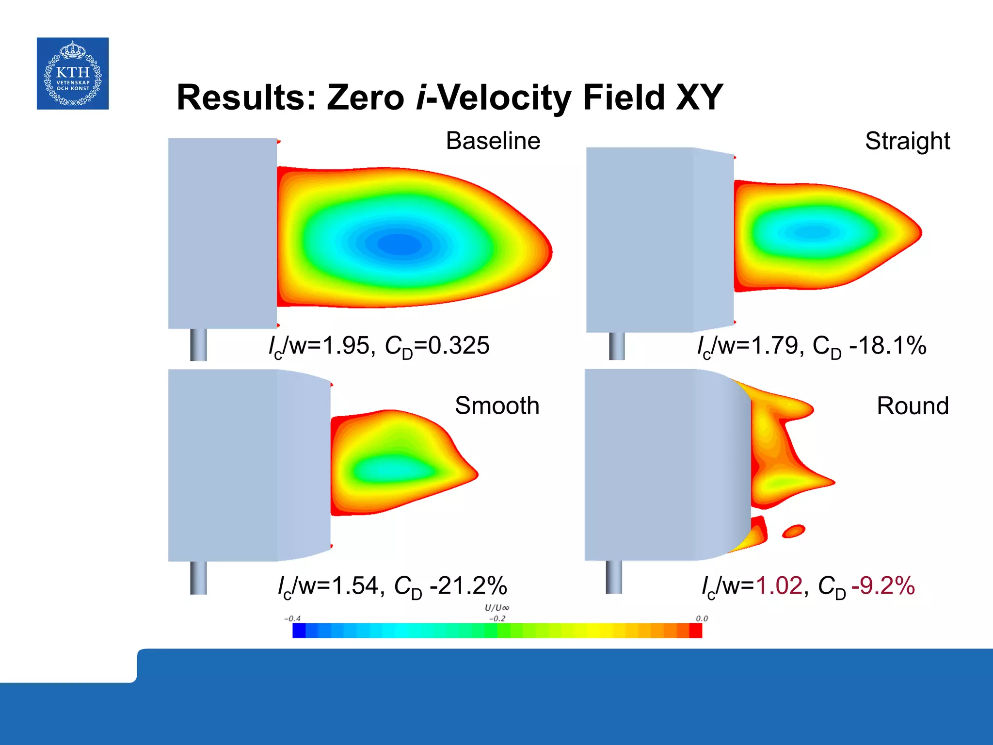
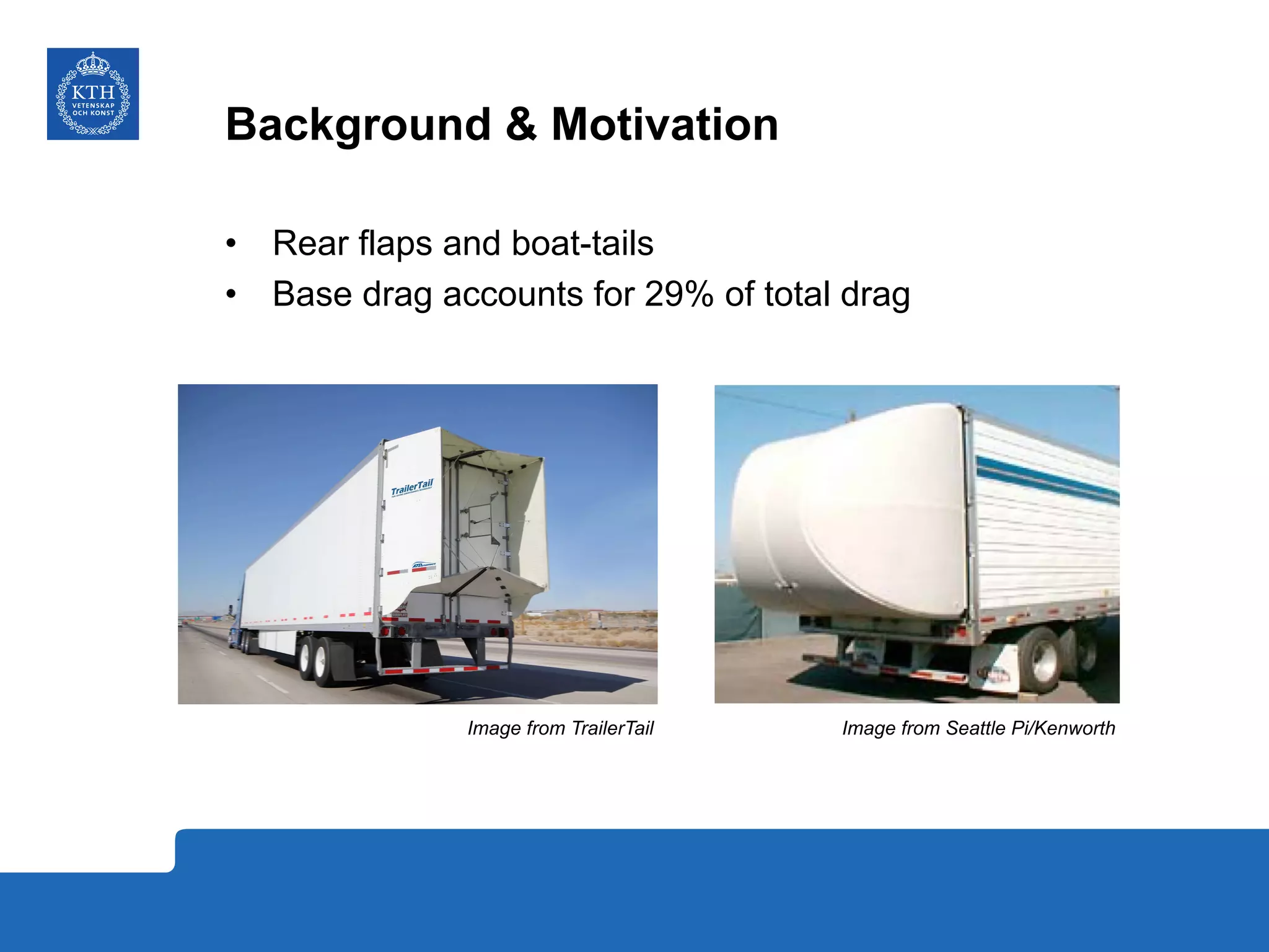
The document summarizes a numerical analysis of improving the aerodynamic performance of trucks through modifications to the design of the rear section. The analysis used computational fluid dynamics to simulate different boat-tail and rear flap designs. The best design was found to reduce drag by 21.2% compared to the baseline design. Further work is recommended to better capture unsteady effects and optimize designs for real trucks.


![Forces, coefficients & representative scales
CD =
2FD
ρU2
A
Coefficent of drag
FD = drag force [N]
ρ = fluid density [kg/m3]
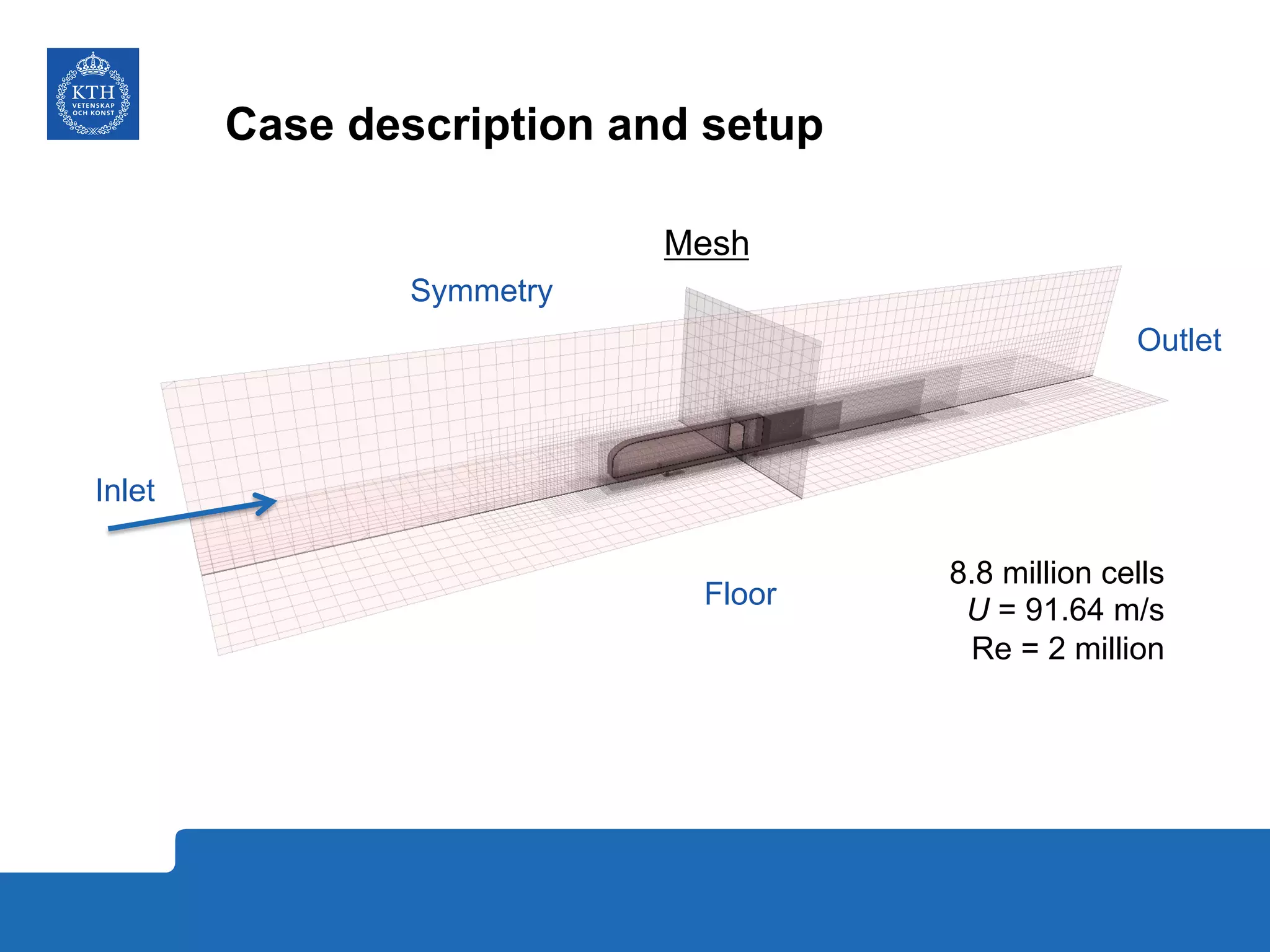
U = freestream velocity [m/s]
A = projected area [m2]](https://image.slidesharecdn.com/f9dcf613-599b-498d-8736-e14baf05cb91-150608162410-lva1-app6892/75/johan_malmberg_thesis_pres_final-15-2048.jpg)
![Forces, coefficients & representative scales
CD =
2FD
ρU2
A
Coefficent of drag
FD = drag force [N]
ρ = fluid density [kg/m3]
U = freestream velocity [m/s]
A = projected area [m2]
Re =
ρUL
µ
Reynolds number
L = characteristic length [m]
µ = dynamic viscosity [PaŸs]](https://image.slidesharecdn.com/f9dcf613-599b-498d-8736-e14baf05cb91-150608162410-lva1-app6892/75/johan_malmberg_thesis_pres_final-16-2048.jpg)