These are notes on Introduction to Statistics. They cover the following concepts :
-Explain the meaning of data and statistics
-Describe the role of uncertainty in decision-making
-distinguish between various terms and concepts utilized in statistical analysis
-distinguish between descriptive and inferential statistics
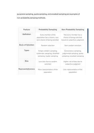
-distinguish between probability and non-probability sampling