Downloaded 1,470 times


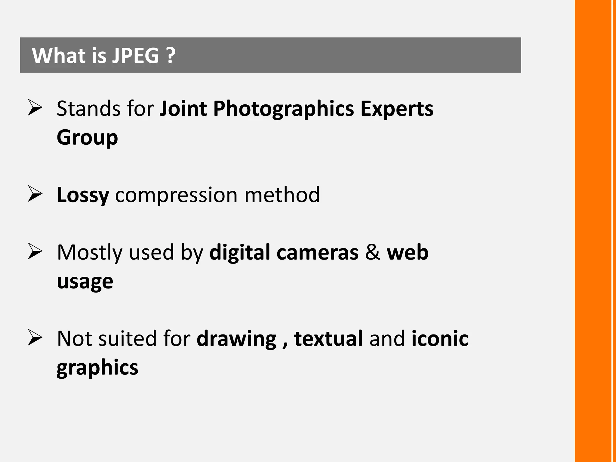
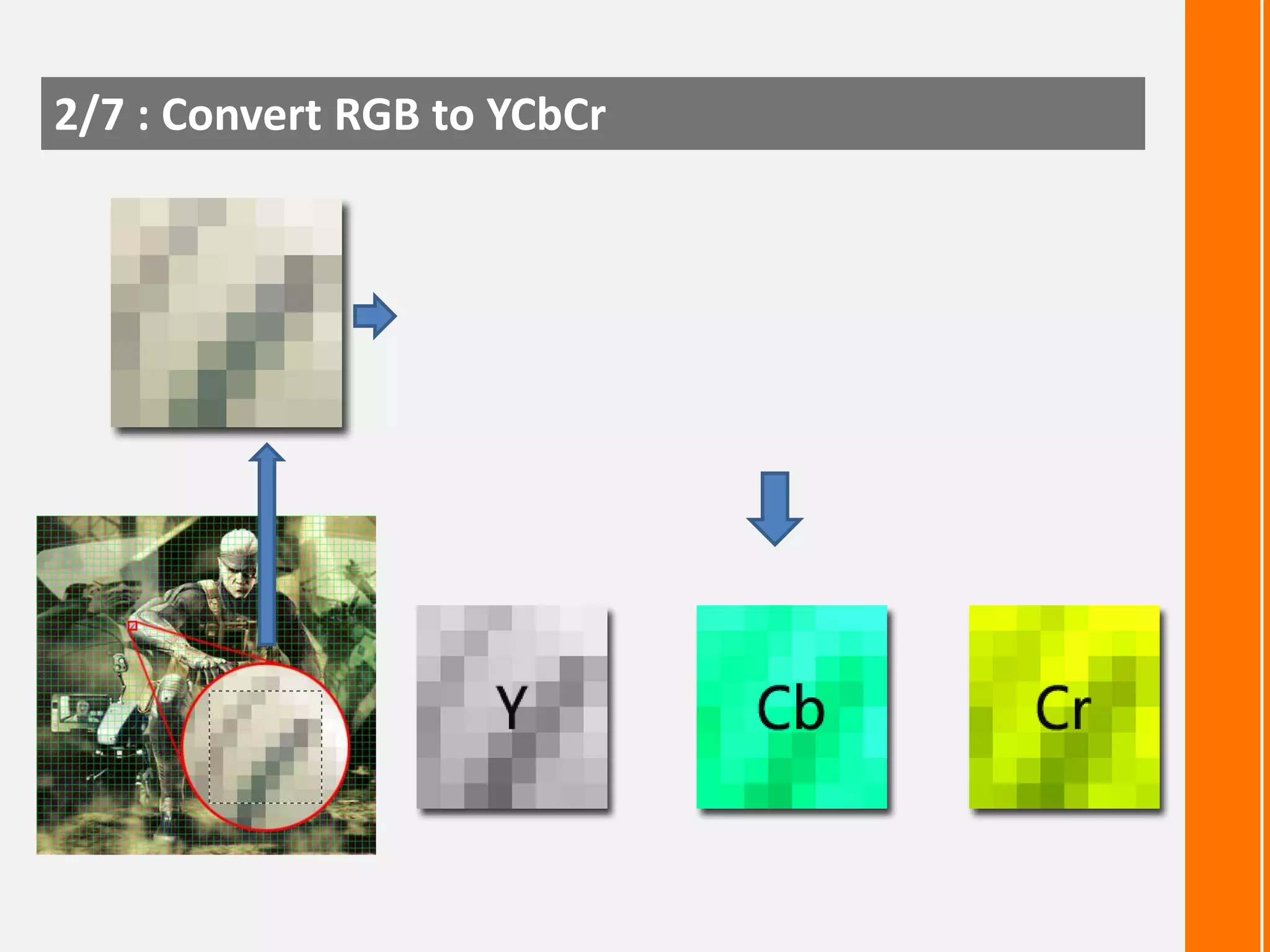
![2/7 : Convert RGB to YCbCr
Simple color space model: [R,G,B] per pixel
JPEG uses [Y, Cb, Cr] Model
Y (Brightness) = 0.299R + 0.587G + 0.114B
Cb (Color blueness) = -0.1687R - 0.3313G + 0.5B + 128
Cr (Color redness) = 0.5R - 0.4187G - 0.0813B + 128](https://image.slidesharecdn.com/imagecompression-131204091956-phpapp01/75/Image-Compression-18-2048.jpg)
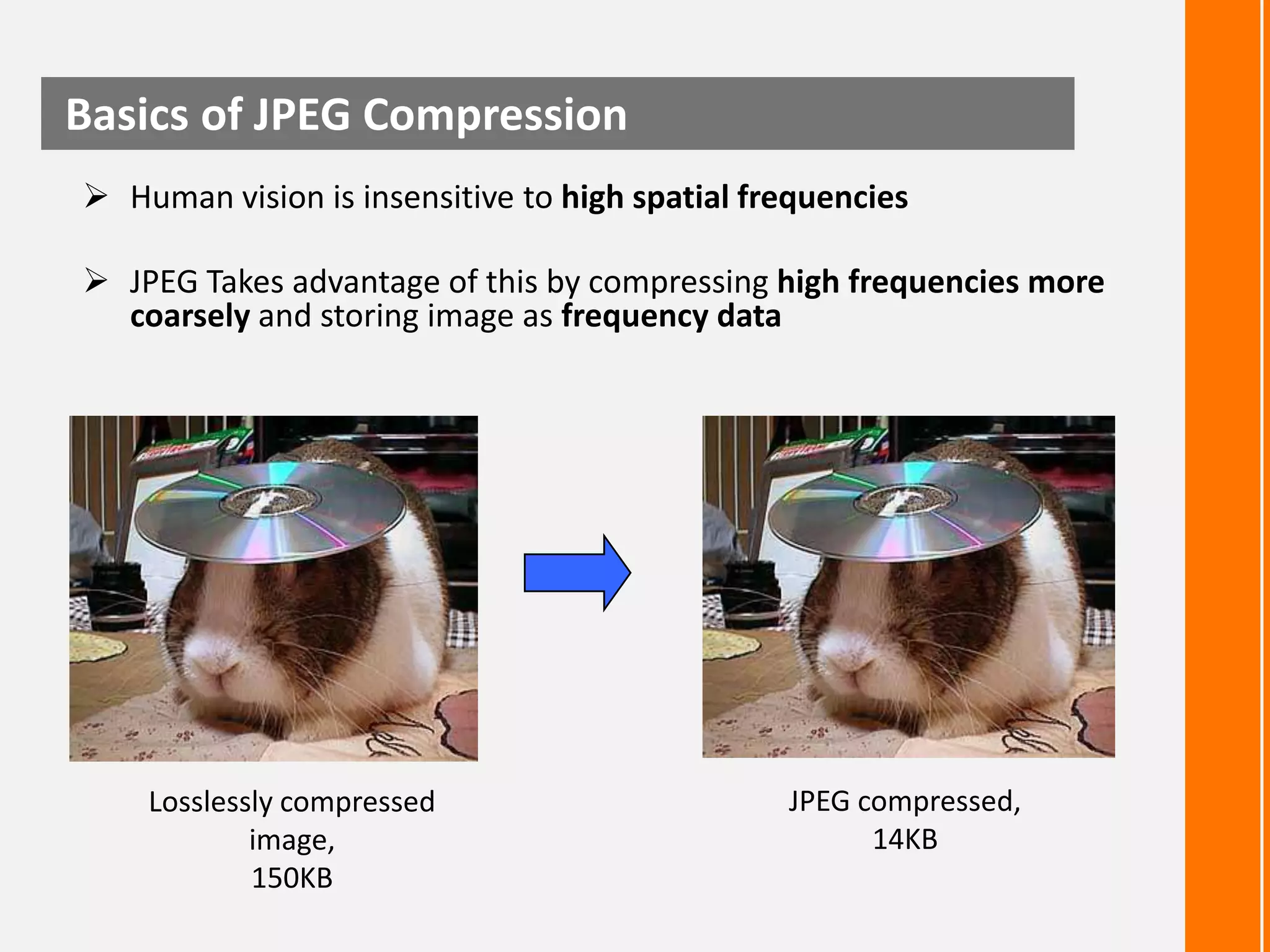
![4/7 : Apply DCT [ Discrete Cosine Transformation ]
2D DCT:
1D DCT:](https://image.slidesharecdn.com/imagecompression-131204091956-phpapp01/75/Image-Compression-21-2048.jpg)
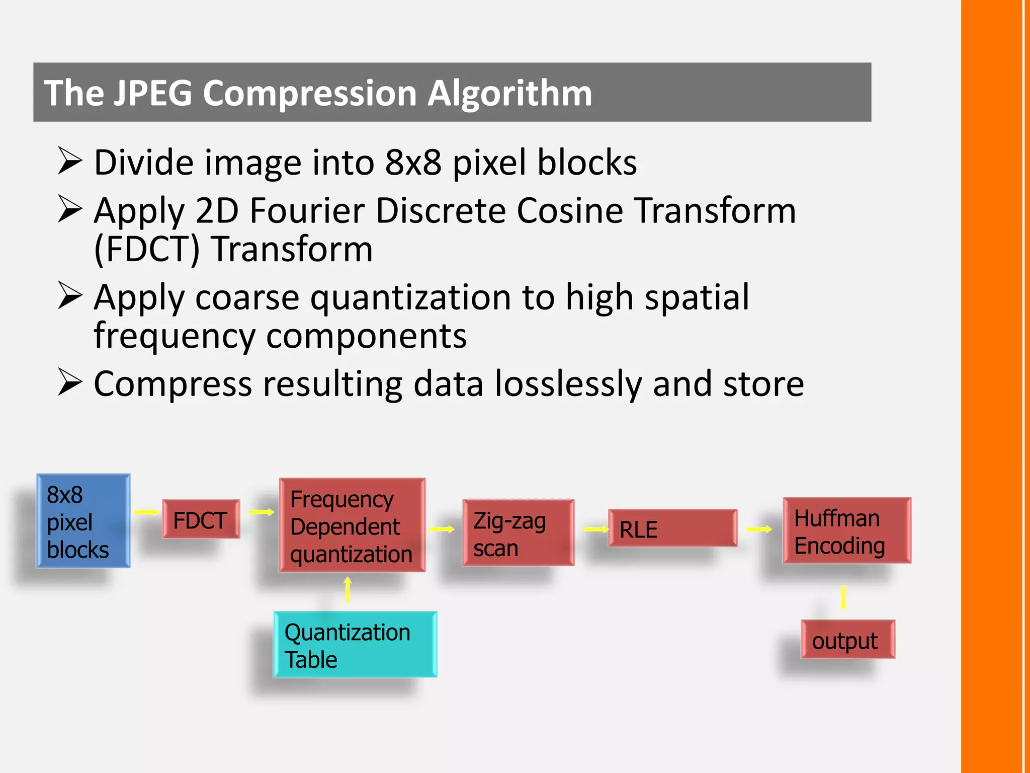
![4/7 : Apply DCT [ Discrete Cosine Transformation ]
Shift operations
From [0, 255]
To [-128, 127]
DCT
Result](https://image.slidesharecdn.com/imagecompression-131204091956-phpapp01/75/Image-Compression-22-2048.jpg)
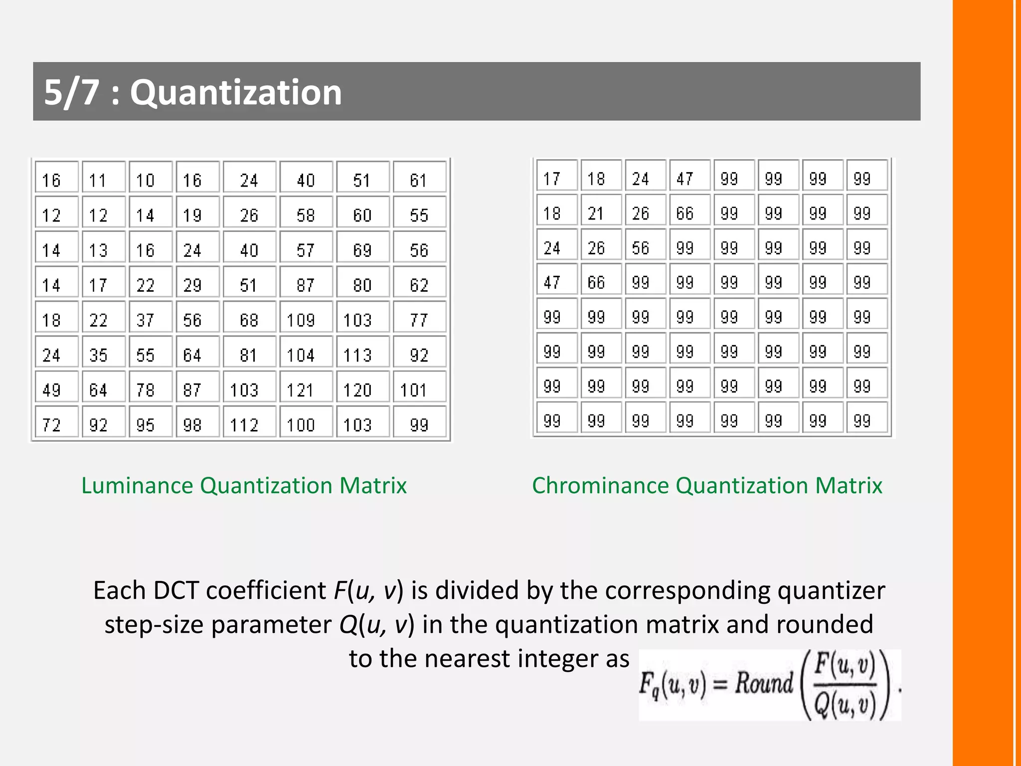
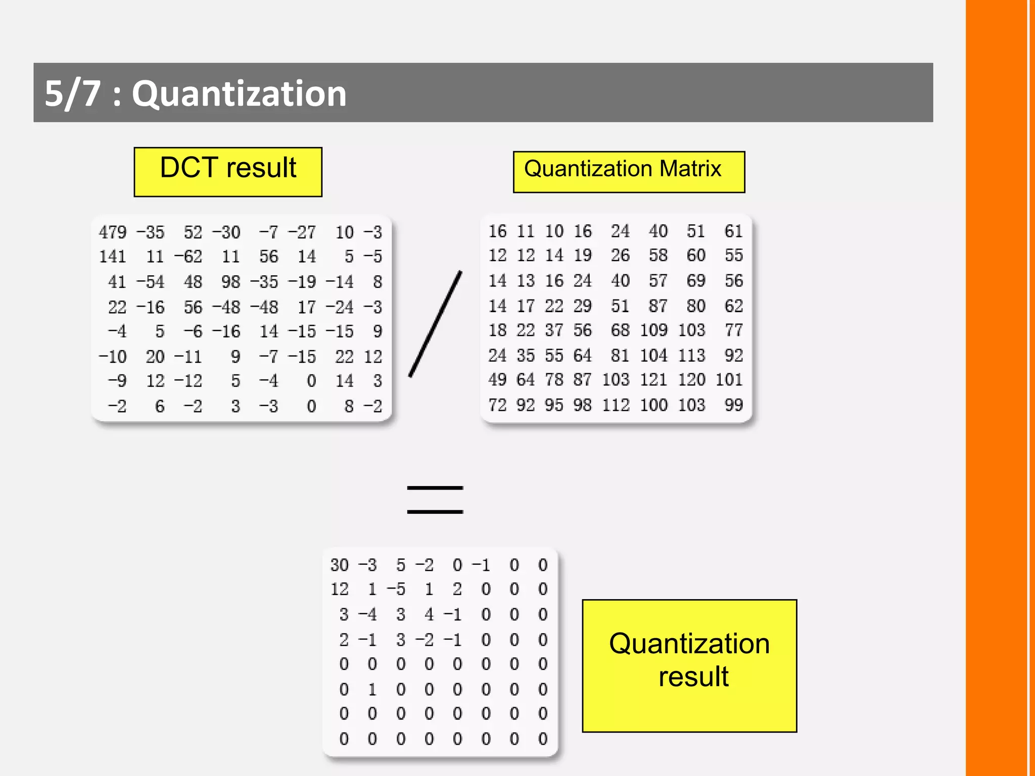
![5/7 : Quantization [ Quality Factor ]
Quality of the reconstructed image and the achieved
compression can be controlled by a user by selecting a
quality factor [ Q_JPEG ] :
Q_JPEG ranges between 1 to 100
When Q_JPEG is used, the entries in tables in previous slide is
scaled by the factor alpha (α), defined as :
Q_JPEG is 100 for best reproduction](https://image.slidesharecdn.com/imagecompression-131204091956-phpapp01/75/Image-Compression-24-2048.jpg)
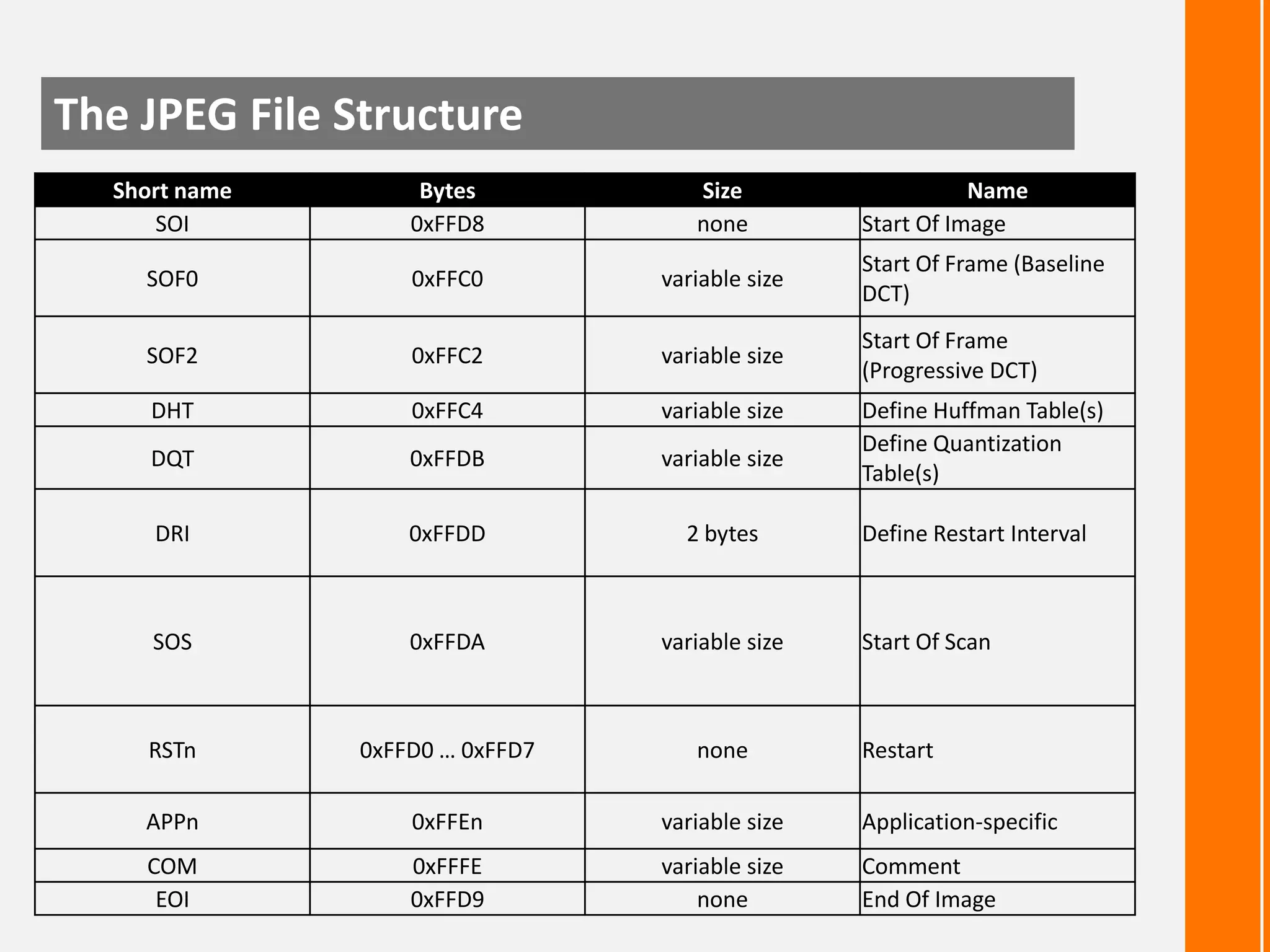
![7/7 : Huffman encoding
Values
G
0
0
-1, 1
1
-3, -2, 2, 3
2
-7,-6,-5,-4,5,6,7 3
.
4
.
5
.
.
.
.
.
.
.
.
.
.
.
.
.
.
-32767..32767 15
Real saved values
.
0,1
00, 01, 10, 11
000,001,010,011,100,101,110,111
.
.
.
.
.
.
.
.
.
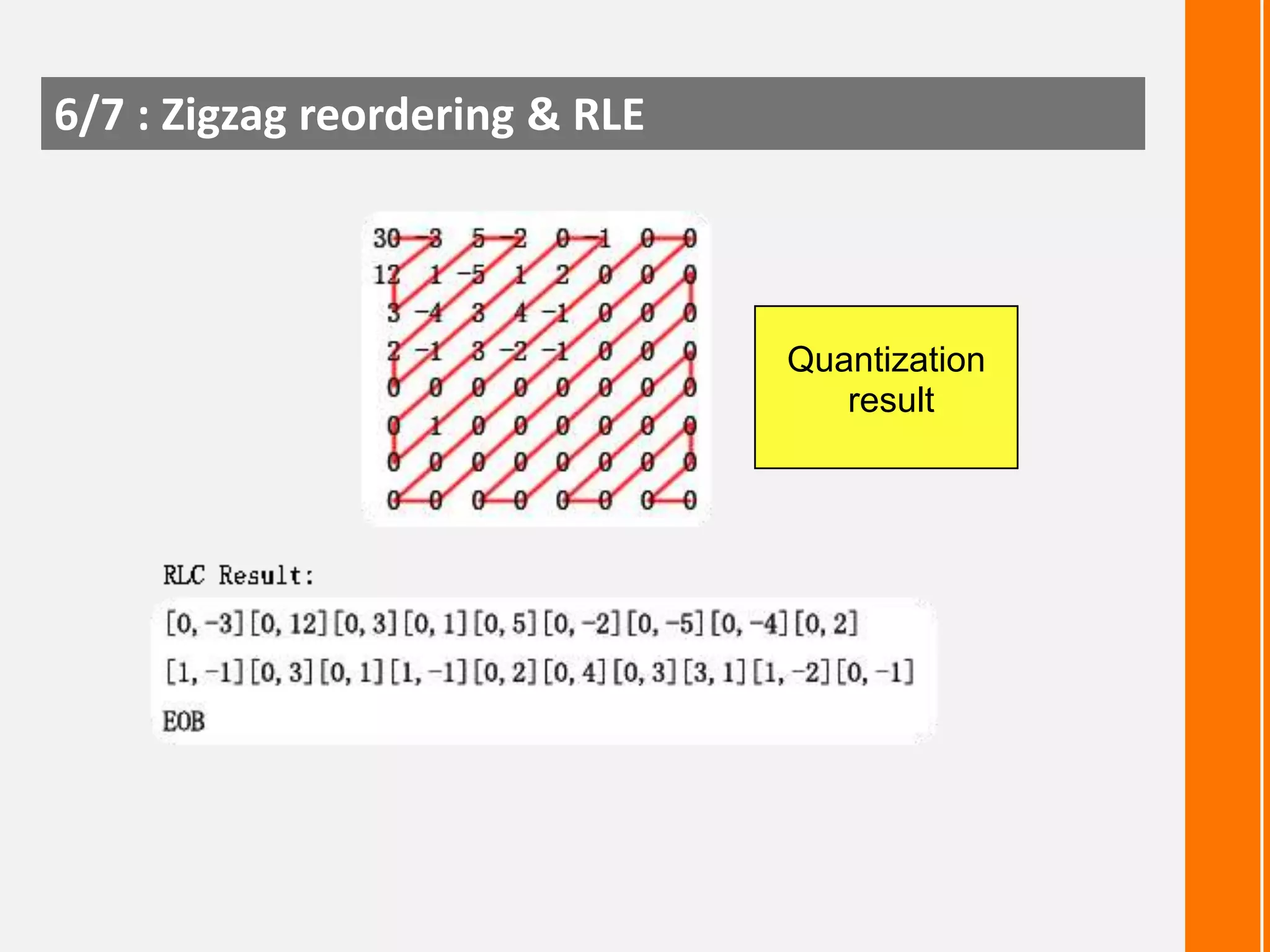
RLC result:
[0, -3] [0, 12] [0,
3]......EOB
After group number added:
[0,2,00b] [0,4,1100b]
[0,2,00b]
...... EOB
First Huffman coding (i.e. for
[0,2,00b] ):
[0, 2, 00b] => [100b,
00b]
Input : 512 bits
Output : 113 bits
% Red : 22.07 %](https://image.slidesharecdn.com/imagecompression-131204091956-phpapp01/75/Image-Compression-27-2048.jpg)
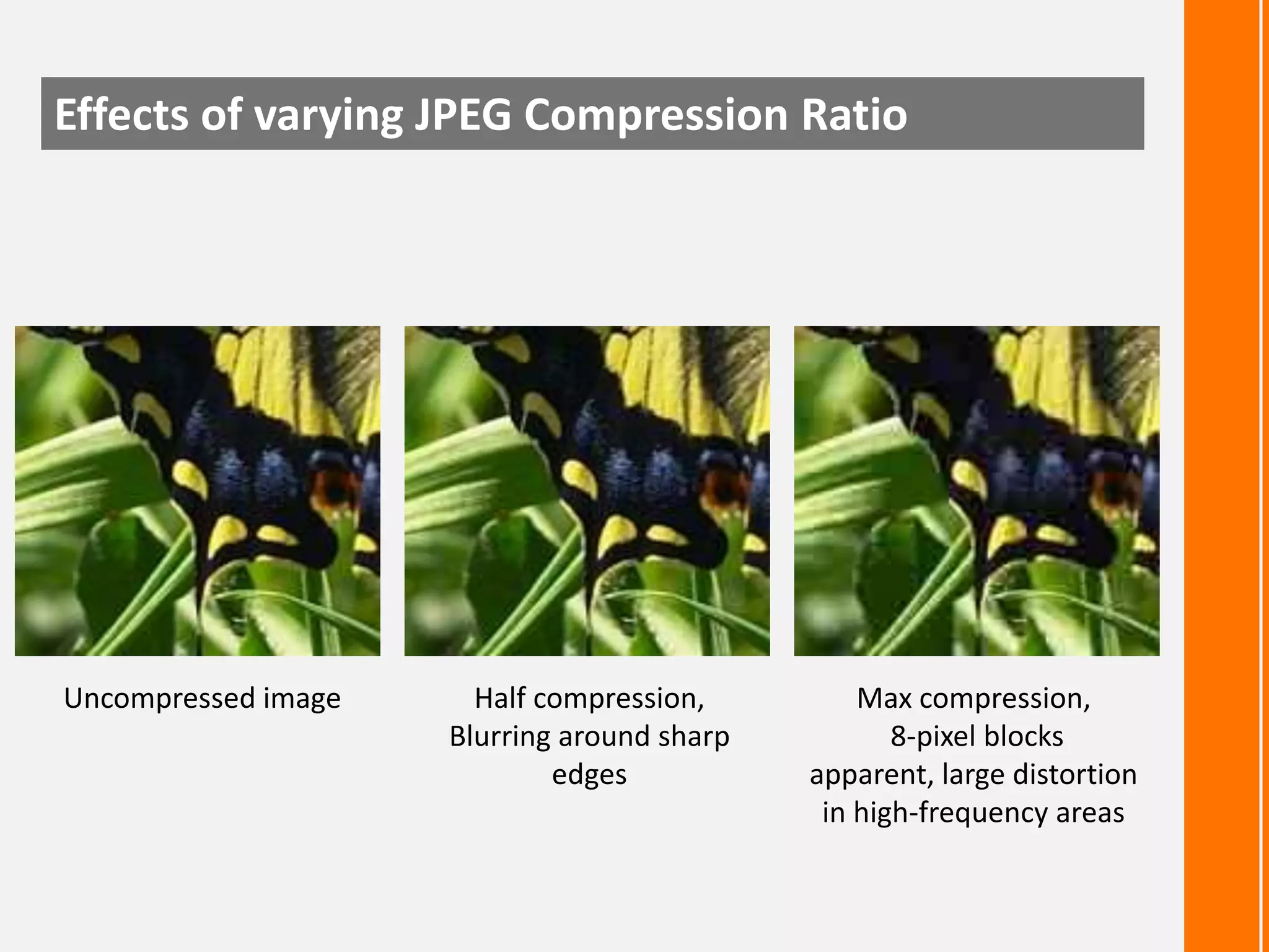
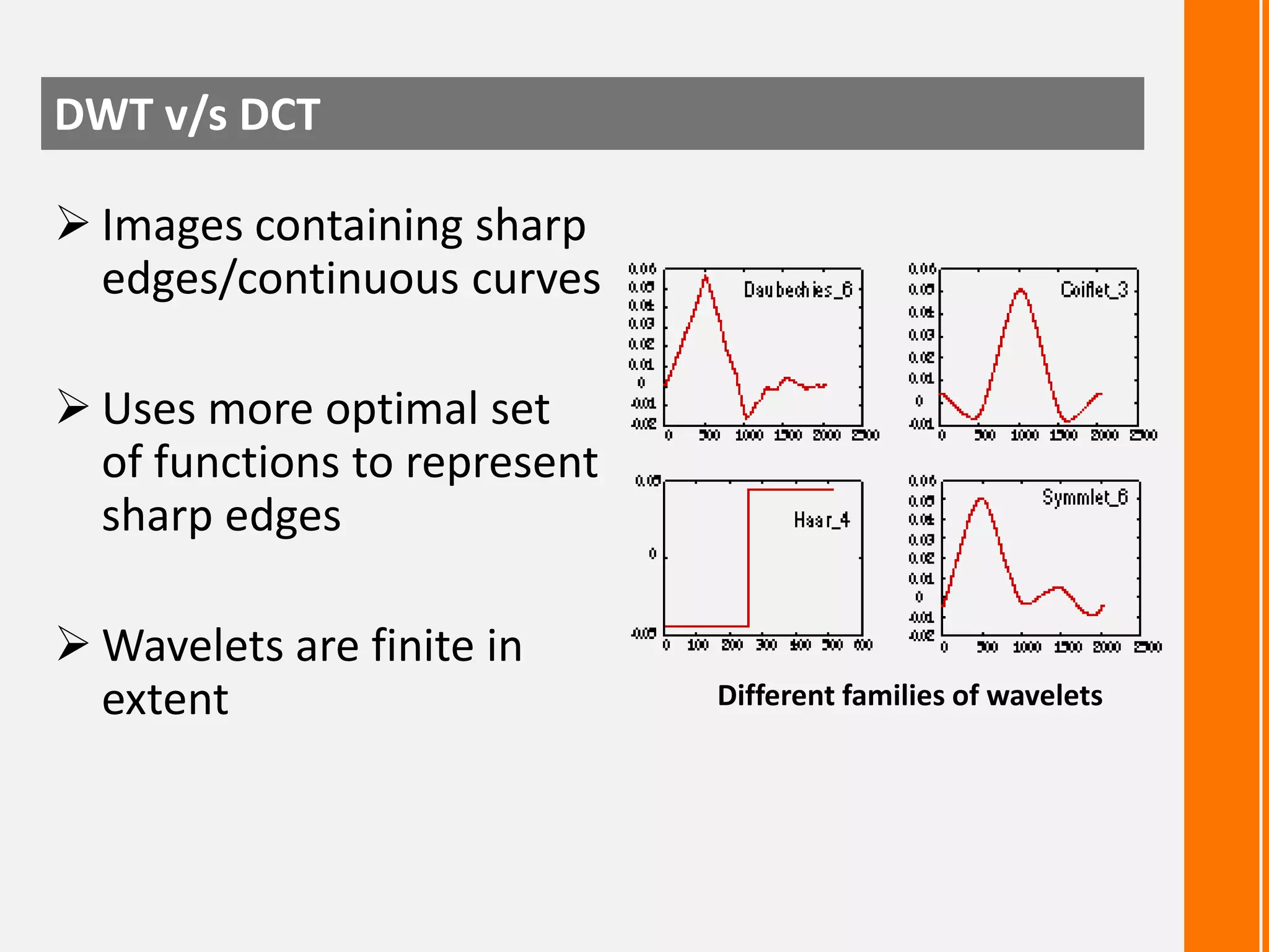
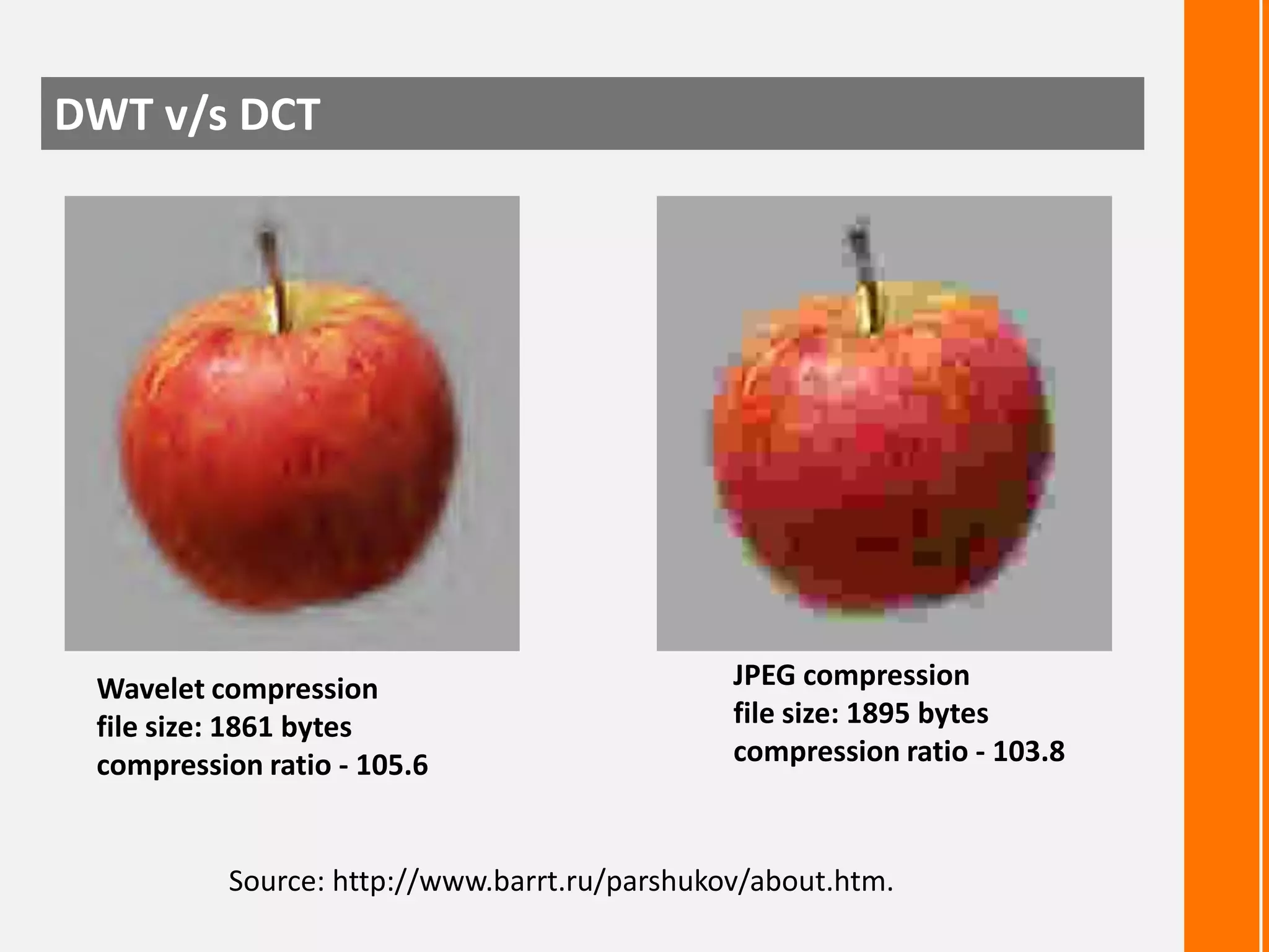
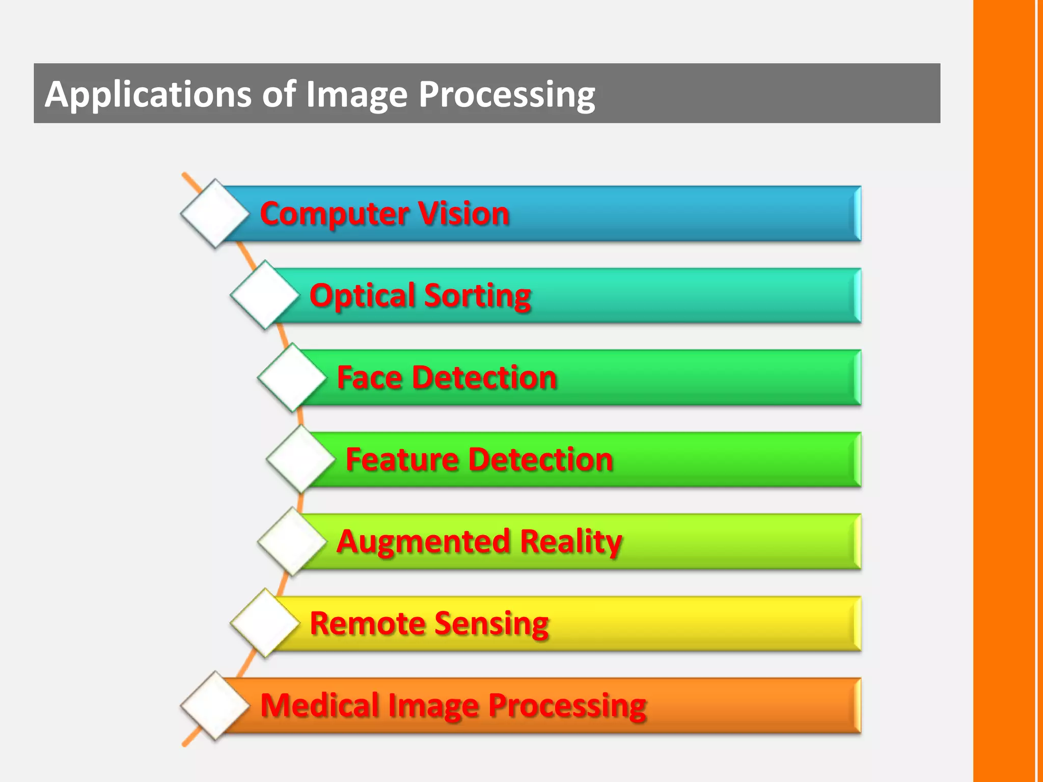
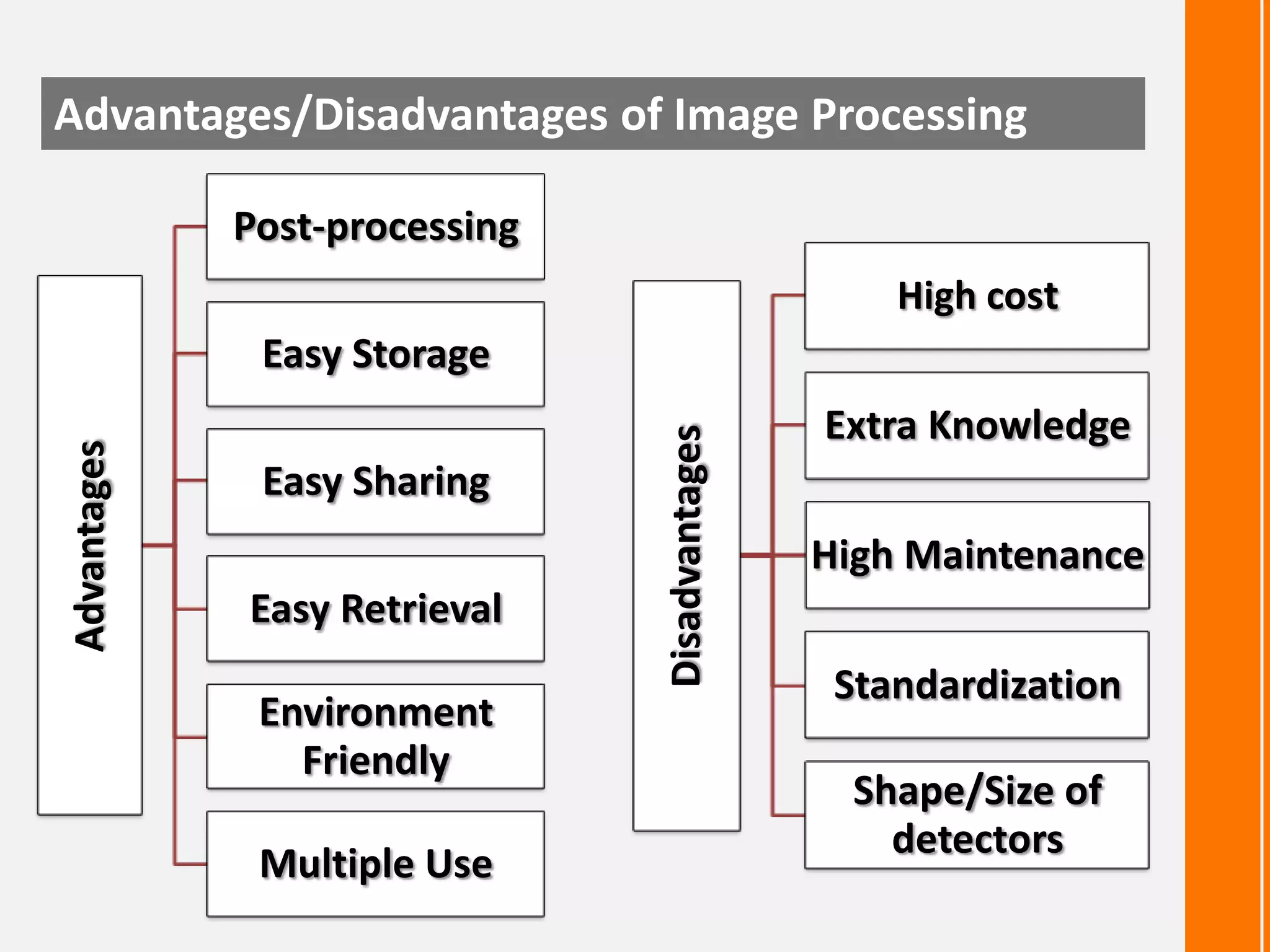


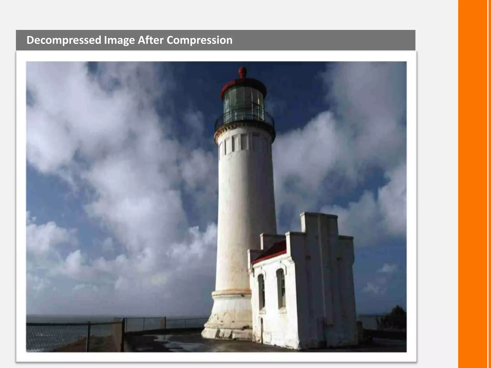
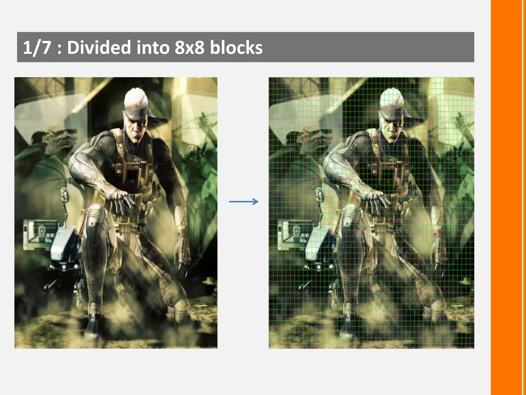
The document discusses image compression techniques in electrical and electronics engineering, detailing lossy and lossless compression methods, specifically focusing on JPEG compression algorithms. It explains concepts like discrete cosine transform (DCT), quantization, and Huffman encoding, along with the practical applications and advantages of image processing. Additionally, it touches upon the comparison between discrete wavelet transform (DWT) and DCT, and lists various applications of image processing in fields like computer vision and medical imaging.