Downloaded 220 times


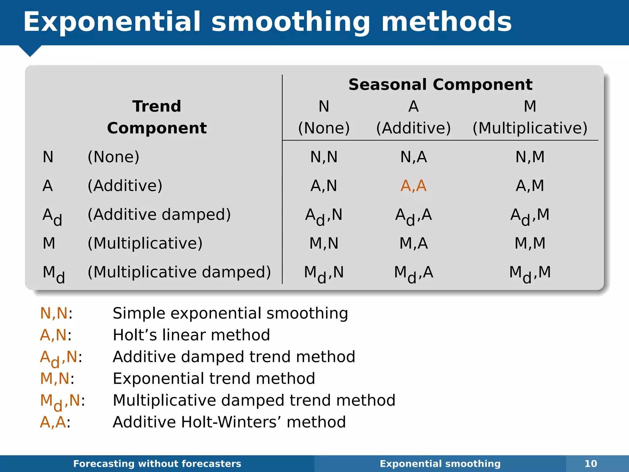


![Auto ARIMA
Forecasting without forecasters ARIMA modelling 23
Forecasts from ARIMA(3,1,3)(0,1,1)[12]
Year
Totalscripts(millions)
1995 2000 2005 2010
0.40.60.81.01.21.4](https://image.slidesharecdn.com/hyndman-rob-isf2013-130703151347-phpapp02/75/Forecasting-without-forecasters-59-2048.jpg)
![Auto ARIMA
fit <- auto.arima(h02)
fcast <- forecast(fit)
plot(fcast)
Forecasting without forecasters ARIMA modelling 24
Forecasts from ARIMA(3,1,3)(0,1,1)[12]
Year
Totalscripts(millions)
1995 2000 2005 2010
0.40.60.81.01.21.4](https://image.slidesharecdn.com/hyndman-rob-isf2013-130703151347-phpapp02/75/Forecasting-without-forecasters-60-2048.jpg)


![Hierarchical data
Total
A B C
Yt = [Yt, YA,t, YB,t, YC,t] =
1 1 1
1 0 0
0 1 0
0 0 1
YA,t
YB,t
YC,t
Forecasting without forecasters Hierarchical and grouped time series 40
Yt : observed aggregate of all
series at time t.
YX,t : observation on series X at
time t.
Bt : vector of all series at
bottom level in time t.](https://image.slidesharecdn.com/hyndman-rob-isf2013-130703151347-phpapp02/75/Forecasting-without-forecasters-93-2048.jpg)
![Hierarchical data
Total
A B C
Yt = [Yt, YA,t, YB,t, YC,t] =
1 1 1
1 0 0
0 1 0
0 0 1
S
YA,t
YB,t
YC,t
Forecasting without forecasters Hierarchical and grouped time series 40
Yt : observed aggregate of all
series at time t.
YX,t : observation on series X at
time t.
Bt : vector of all series at
bottom level in time t.](https://image.slidesharecdn.com/hyndman-rob-isf2013-130703151347-phpapp02/75/Forecasting-without-forecasters-94-2048.jpg)
![Hierarchical data
Total
A B C
Yt = [Yt, YA,t, YB,t, YC,t] =
1 1 1
1 0 0
0 1 0
0 0 1
S
YA,t
YB,t
YC,t
Bt
Forecasting without forecasters Hierarchical and grouped time series 40
Yt : observed aggregate of all
series at time t.
YX,t : observation on series X at
time t.
Bt : vector of all series at
bottom level in time t.](https://image.slidesharecdn.com/hyndman-rob-isf2013-130703151347-phpapp02/75/Forecasting-without-forecasters-95-2048.jpg)
![Hierarchical data
Total
A B C
Yt = [Yt, YA,t, YB,t, YC,t] =
1 1 1
1 0 0
0 1 0
0 0 1
S
YA,t
YB,t
YC,t
Bt
Yt = SBt
Forecasting without forecasters Hierarchical and grouped time series 40
Yt : observed aggregate of all
series at time t.
YX,t : observation on series X at
time t.
Bt : vector of all series at
bottom level in time t.](https://image.slidesharecdn.com/hyndman-rob-isf2013-130703151347-phpapp02/75/Forecasting-without-forecasters-96-2048.jpg)


![Example using R
library(hts)
# bts is a matrix containing the bottom level time series
# g describes the grouping/hierarchical structure
y <- hts(bts, g=c(1,1,2,2))
# Forecast 10-step-ahead using optimal combination method
# ETS used for each series by default
fc <- forecast(y, h=10)
# Select your own methods
ally <- allts(y)
allf <- matrix(, nrow=10, ncol=ncol(ally))
for(i in 1:ncol(ally))
allf[,i] <- mymethod(ally[,i], h=10)
allf <- ts(allf, start=2004)
# Reconcile forecasts so they add up
fc2 <- combinef(allf, Smatrix(y))
Forecasting without forecasters Hierarchical and grouped time series 47](https://image.slidesharecdn.com/hyndman-rob-isf2013-130703151347-phpapp02/75/Forecasting-without-forecasters-116-2048.jpg)


This document outlines an approach for automatic time series forecasting without human forecasters. It discusses the need for algorithms that can determine appropriate models, estimate parameters, and generate forecasts for large numbers of time series across different domains. Exponential smoothing methods and ARIMA models are covered as approaches that can be used for automatic forecasting if enhanced with techniques for model selection, parameter estimation, and producing prediction intervals. The document also motivates this work by noting limitations in previous research on general automatic forecasting algorithms.


![time series.ppt [Autosaved].pdf](https://cdn.slidesharecdn.com/ss_thumbnails/timeseries-231013231623-6993e801-thumbnail.jpg?width=640&height=640&fit=bounds)