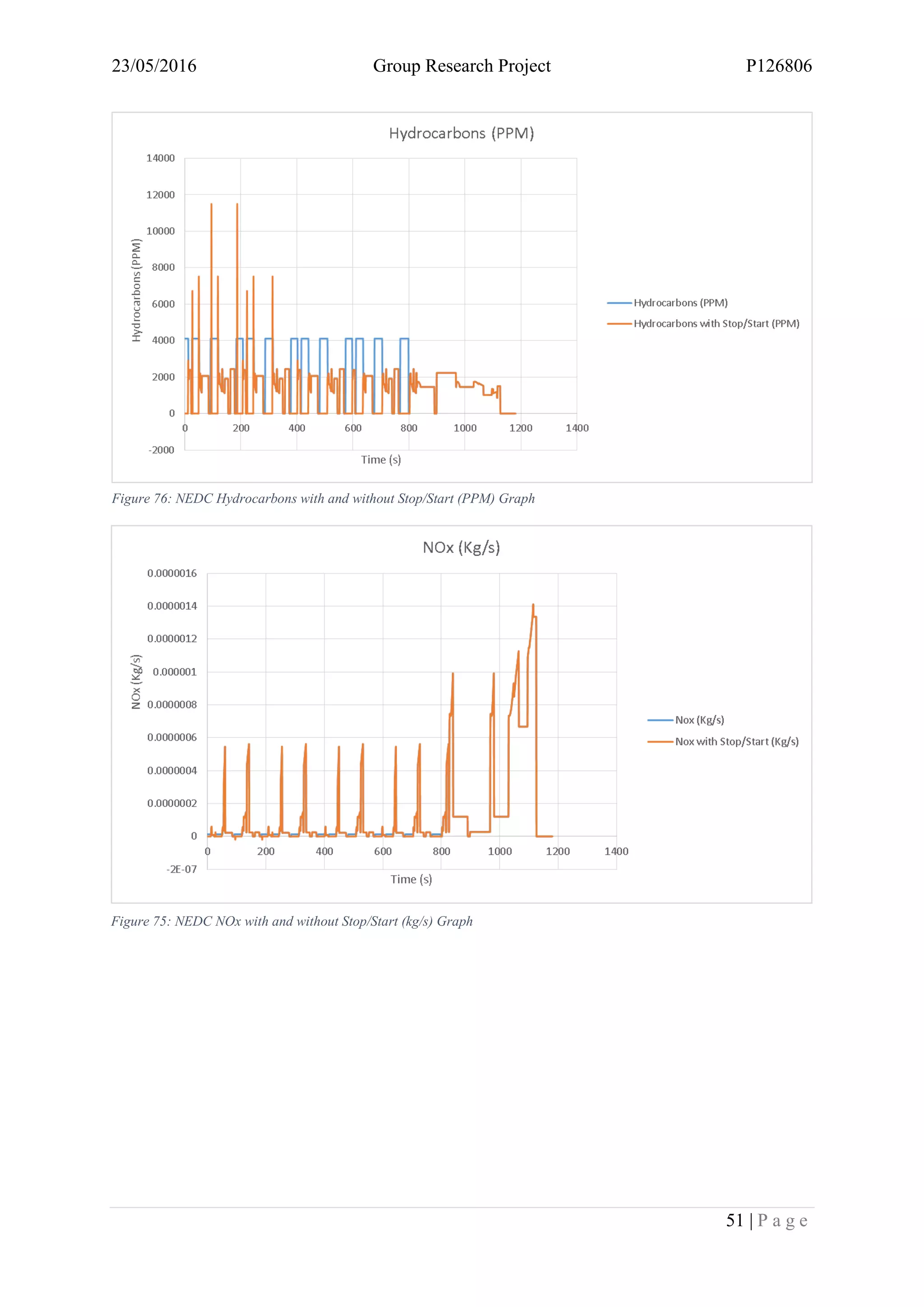
SlideShare a Scribd company logo
1 of 99
Download to read offline
University of Wales: Trinity St. David Swansea
MEng Motorcycle Engineering
GROUP RESEARCH PROJECT
By Jack Saunders
23/05/2016 Group Research Project P126806
1 | P a g e
Figure 1: NEDC Velocity (m/s) Graph....................................................................................12
Figure 2: NEDC Selected Gear Graph.....................................................................................12
Figure 3: NEDC Force Due to Acceleration Graph.................................................................13
Figure 4: NEDC Vehicle Acceleration Graph .........................................................................13
Figure 5: NEDC Aerodynamic Drag Force .............................................................................14
Figure 6: NEDC Force Due to Acceleration with Energy Recovery Graph............................14
Figure 7: NEDC Drive Force Graph........................................................................................15
Figure 8: NEDC Rolling Resistance Force Graph...................................................................15
Figure 9: NEDC Wheel Torque Graph ....................................................................................16
Figure 10: NEDC Drive Force with Energy Recovery Graph.................................................16
Figure 11: NEDC Wheel Speed (RPM) Graph........................................................................17
Figure 12: NEDC Prop Shaft Torque Graph............................................................................17
Figure 13: NEDC Engine Torque (Nm) Graph........................................................................18
Figure 14: NEDC Engine Speed (RPM) Graph.......................................................................18
Figure 15: NEDC Dynometer Torque (Nm) Graphs ...............................................................19
Figure 16: NEDC Engine Angular Acceleration (Rad/sΒ²) Graph ............................................19
Figure 17: NEDC Energy Generated with Energy Recovery (J/s) Graph ...............................20
Figure 18: NEDC Energy Generated (J/s) Graph ....................................................................20
Figure 19: NEDC Engine Speed from Data (RPM) Graph......................................................21
Figure 20: NEDC Fuel Mass (g/s) Graph ................................................................................21
Figure 21: NEDC Fuel Mass with Stop/Start (g/s) Graph .......................................................22
Figure 22: NEDC Engine Speed from Data with Stop/Start (RPM) Graph ............................22
Figure 23: NEDC NOx (PPM) Graph......................................................................................23
Figure 24: NEDC Hydrocarbons (PPM) Graph.......................................................................23
Figure 25: NEDC NOx (Kg/s) Graph ......................................................................................24
Figure 26: NEDC NOx with Stop/Start (PPM) Graph ............................................................24
Figure 27: NEDC NOx with Stop/Start (Kg/s) Graph.............................................................25
Figure 28: Drive Force IF Statement .......................................................................................26
Figure 29: Engine Speed IF Statement ....................................................................................27
Figure 30: Idle IF Statement ....................................................................................................28
Figure 31: Engine Torque IF Statement...................................................................................28
Figure 32: RPM lookup ...........................................................................................................29
Figure 33: Index Drive Cycle NEDC.......................................................................................29
Figure 34: RPM Match ............................................................................................................29
Figure 35: Index Match Result NEDC.....................................................................................29
Figure 36: WLTP Gear Selected Graph...................................................................................31
Figure 37: WLTP Vehicle Velocity (m/s) Graph ....................................................................31
Figure 38: WLTP Force due to Acceleration (N) ....................................................................32
Figure 39: WLTP Vehicle Acceleration (m/sΒ²) Graph.............................................................32
Figure 40: WLTP Aerodynamic Drag Force (N) Graph..........................................................33
Figure 41: WLTP Force due to Acceleration with Energy Recovery (N) Graph ....................33
Figure 42: WLTP Drive Force (N) Graph ...............................................................................34
Figure 43: WLTP Rolling Resistance Force (N) Graph ..........................................................34
Figure 44: WLTP Wheel Torque (Nm) Graph ........................................................................35
Figure 45: WLTP Drive Force with Energy Recovery (N) Graph ..........................................35
Figure 46: WLTP Wheel Speed (RPM) Graph........................................................................36
23/05/2016 Group Research Project P126806
2 | P a g e
Figure 47: WLTP Propshaft Torque (Nm) Graph....................................................................36
Figure 48: WLTP Engine Torque (Nm) Graph........................................................................37
Figure 49: WLTP Engine Speed (RPM) Graph.......................................................................37
Figure 50: WLTP Dynometer Torque (Nm) Graph.................................................................38
Figure 51: WLTP Engine Angular Acceleration (Rad/sΒ²) Graph ............................................38
Figure 52: WLTP Energy Generated per Second (J/s) Graph .................................................39
Figure 53: WLTP Energy Generated per Second (J/s) Graph .................................................39
Figure 54: WLTP Engine Speed with Stop/Start (RPM) Graph..............................................40
Figure 55: WLTP Engine Speed from Data (RPM) Graph......................................................40
Figure 56: WLTP Fuel Mass with Stop/Start (g/s) Graph .......................................................41
Figure 57: WLTP Fuel Mass (g/s) Graph ................................................................................41
Figure 58: WLTP Hydrocarbons with Stop/Start (PPM) Graph..............................................42
Figure 59: WLTP Hydrocarbons (PPM) Graph.......................................................................42
Figure 60: WLTP NOx with Stop/Start (PPM) Graph ............................................................43
Figure 61: WLTP NOx (PPM) Graph......................................................................................43
Figure 62: WLTP NOx with Stop/Start (Kg/s) Graph.............................................................44
Figure 63: WLTP NOx (Kg/s) Graph ......................................................................................44
Figure 64: Drive Force IF Statement .......................................................................................45
Figure 65: Engine Speed IF Statement ....................................................................................46
Figure 66: Idle Speed Correction.............................................................................................47
Figure 67: Engine Torque IF Statements.................................................................................47
Figure 68: Drive Cycle Lookup WLTP ...................................................................................48
Figure 69: Drive Cycle Index WLTP.......................................................................................48
Figure 70: Drive Cycle Match WLTP .....................................................................................48
Figure 71: Index Match WLTP................................................................................................48
Figure 72: Total Fuel Required................................................................................................48
Figure 73: NEDC Fuel Mass with and without Stop/Start Graph ...........................................50
Figure 74: NEDC RPM with and without Stop/Start Graph....................................................50
Figure 75: NEDC NOx with and without Stop/Start (kg/s) Graph..........................................51
Figure 76: NEDC Hydrocarbons with and without Stop/Start (PPM) Graph..........................51
Figure 77: NEDC vs. WLTP Velocity (m/s) Graph ................................................................52
Figure 78: NEDC Vs. WLTP - MPG.......................................................................................53
Figure 79: NOx Production NEDC Vs. WLTP .......................................................................54
Figure 80: Piston Displacements with Varying Offsets (m) Graph.........................................56
Figure 81: Connecting Rod Angle with Varying Offsets Graph .............................................56
Figure 82: Piston Acceleration Graph......................................................................................57
Figure 83: Piston Velocity (m/Degree) Graph.........................................................................57
Figure 84: Cylinder Pressure (Bar) Graph...............................................................................58
Figure 85: Inertia Force (N) with varying Offsets Graph........................................................58
Figure 86: Net Force (N) with varying offsets Graph..............................................................59
Figure 87: Gas Force (N) Graph ..............................................................................................59
Figure 88: Work Done (J/s) with varying Offsets Graph ........................................................60
Figure 89: Side Friction Force (N) with varying Offsets Graph..............................................60
Figure 90: FMEP Piston Skirt 0->12mm Crankshaft Offset Graph ........................................63
Figure 91: Actual Bank Angle due to Offset ...........................................................................66
Figure 92: Bank 1 Connecting Rod Length .............................................................................66
23/05/2016 Group Research Project P126806
3 | P a g e
Figure 93: Bank 2 Connecting Rod Equation..........................................................................66
Figure 94: V-Twin MCrankspan* X Bank 1 Equation............................................................67
Figure 95: V-Twin MCrankspan* X Bank 2 Equation............................................................67
Figure 96: V-Twin Offset Centre of Mass Angle - Bank 1 .....................................................67
Figure 97: V-Twin Offset Centre of Mass Angle - Bank 2 .....................................................67
Figure 98: V-Twin MBalance*Y - Bank 1 ..............................................................................68
Figure 99: V-Twin MBalance*Y - Bank 2 ..............................................................................68
Figure 100: Offset centre of mass angle - V Twin - Balance Shaft - Bank 1 ..........................68
Figure 101: Offset Centre of Mass Angle - Bank 2.................................................................68
Figure 102: Single Cylinder Crankshaft MCrank*X (Kgm) Graph ........................................69
Figure 103: Single Cylinder Balance Shaft - MBalance*Y (Kgm) Graph ..............................70
Figure 104: Single Cylinder Balance Shaft Offset Centre of Mass (Degrees) Graph .............71
Figure 105: Single Cylinder Crankshaft Offset Centre of Mass Angle (Degrees) Graph .......71
Figure 106: Connecting Rod Length (m) - 60 Degree Bank Angle.........................................72
Figure 107: Connecting Rod Length (m) - 45 Degree Bank Angle.........................................72
Figure 108: Connecting Rod Length (m) - 90 Degree Bank Angle.........................................73
Figure 109: Connecting Rod Length (m) - 75 Degree Bank Angle.........................................73
Figure 110: Connecting Rod Length (m) - 110 Degree Bank Angle.......................................74
Figure 111: V-Twin MCrankspan*X Centre of Mass .............................................................75
Figure 112: Cylinder Volume (m) Graph ................................................................................78
Figure 113: Cylinder Pressure (Bar) Graph.............................................................................78
Figure 114: Mass Fraction Burned Graph ...............................................................................79
Figure 115: Difference in pressure, non-combustion to combustion at each degree of crank
angle Graph..............................................................................................................................79
Figure 116: Air Mass Per Revolution (Kg) Graph...................................................................80
Figure 117: Air Mass (Kg/Hr) Graph ......................................................................................80
Figure 118: Fuel Mass Per Cycle (Kg) Graph .........................................................................81
Figure 119: Air Mass Per Cycle (Kg) Graph...........................................................................81
Figure 120: Work Done by Pressure Per Degree (J/Degree)...................................................82
Figure 121: QTotal - Total Energy Released (J) Graph...........................................................82
Figure 122: Change in Energy Release per Degree (J/Degree) Graph ....................................83
Figure 123: Difference in pressure combustion to non-combustion at each degree Equation 83
Figure 124: MFB Equation......................................................................................................83
Figure 125: Air Mass per Revolution Equation.......................................................................83
Figure 126: Air Mass per Cycle Equation ...............................................................................83
Figure 127: Fuel Mass per Cycle Equation..............................................................................84
Figure 128: QTotal Equation ...................................................................................................84
Figure 129: IMEP Standard->10 Degree Advanced................................................................85
Figure 130: NEDC Model #2...................................................................................................88
Figure 131: NEDC Model #1...................................................................................................88
Figure 132: NEDC #4 ..............................................................................................................89
Figure 133: NEDC #3 ..............................................................................................................89
Figure 134: NEDC 6 ................................................................................................................90
Figure 135: NEDC #5 ..............................................................................................................90
Figure 136: WLTP #2 ..............................................................................................................91
Figure 137:WLTP #1 ...............................................................................................................91
23/05/2016 Group Research Project P126806
4 | P a g e
Figure 138: WLTP #4 ..............................................................................................................92
Figure 139: WLTP #3 ..............................................................................................................92
Figure 140: WLTP #6 ..............................................................................................................93
Figure 141: WLTP #5 ..............................................................................................................93
Figure 142: Torque Interpolations ...........................................................................................94
Figure 143: Fuel Mass Interpolations ......................................................................................94
Figure 144: Hydrocarbons Interpolation..................................................................................95
Figure 145: NOx Interpolations...............................................................................................95
Figure 146: Drive Cycle Results..............................................................................................96
Figure 147: Piston FMEP ........................................................................................................97
Figure 148: Ignition Advance Results .....................................................................................97
Figure 149: Crankshaft Balancing #2 ......................................................................................98
Figure 150: Crankshaft Balancing ...........................................................................................98
23/05/2016 Group Research Project P126806
5 | P a g e
Equation 1: NEDC Acceleration Equation ..............................................................................26
Equation 2: NEDC Force of Vehicle Equation........................................................................26
Equation 3: NEDC Aerodynamic Drag Force Equation..........................................................26
Equation 4: Rolling Resistance Force Equation ......................................................................26
Equation 5: Drive Force Equation ...........................................................................................26
Equation 6: Rolling Tyre Radius .............................................................................................27
Equation 7: Wheel Torque Formula ........................................................................................27
Equation 8: Prop Shaft Torque Formula..................................................................................27
Equation 9: Wheel Speed (RPM) Formula ..............................................................................27
Equation 10: Engine Speed (RPM) Equation ..........................................................................27
Equation 11: Engine Torque Formula......................................................................................28
Equation 12: Engine Angular Acceleration Formula...............................................................28
Equation 13: Energy Required per Second Formula ...............................................................28
Equation 14: Fuel Required .....................................................................................................29
Equation 15: Fuel Required (L) Formula.................................................................................30
Equation 16: Fuel Required for 100Km Equation...................................................................30
Equation 17: MPG ...................................................................................................................30
Equation 18: NOx Kmol/S Produced (Kmol/s) .......................................................................30
Equation 19: NOx Kg per Second Equation............................................................................30
Equation 20: Acceleration of Vehicle......................................................................................45
Equation 21: Force of Vehicle .................................................................................................45
Equation 22: Aerodynamic Drag Force ...................................................................................45
Equation 23: Rolling Resistance Force....................................................................................45
Equation 24: Drive Force.........................................................................................................45
Equation 25: Rolling Tyre Radius ...........................................................................................46
Equation 26: Wheel Torque.....................................................................................................46
Equation 27: Prop Shaft Torque ..............................................................................................46
Equation 28: Wheel Speed (RPM)...........................................................................................46
Equation 29: Engine Speed (RPM)..........................................................................................46
Equation 30: Engine Torque....................................................................................................47
Equation 31: Engine Angular Acceleration .............................................................................47
Equation 32: Energy Required per Second..............................................................................47
Equation 33: Fuel Required in Litres.......................................................................................49
Equation 34: Fuel Required in Litres.......................................................................................49
Equation 35: MPG ...................................................................................................................49
Equation 36: NOx Kmol per Second .......................................................................................49
Equation 37: NOx Kg Per Second ...........................................................................................49
Equation 38: Connecting Rod Angle with Offset Equation.....................................................61
Equation 39: Piston Displacement Equation............................................................................61
Equation 40: Piston Velocity Equation....................................................................................61
Equation 41: Piston Acceleration Equation .............................................................................61
Equation 42: Gas Force Equation ............................................................................................61
Equation 43: Inertia Force Equation........................................................................................61
Equation 44: Net Force Equation.............................................................................................61
Equation 45: Connecting Rod Force Equation ........................................................................62
Equation 46: Side Force Equation ...........................................................................................62
23/05/2016 Group Research Project P126806
6 | P a g e
Equation 47: Side Friction Force Equation..............................................................................62
Equation 48: Work Done per Degree Equation .......................................................................62
Equation 49: FMEP (Bar) Equation.........................................................................................62
Equation 50: MRot Equation ...................................................................................................65
Equation 51: MRec Equation...................................................................................................65
Equation 52: MCrankspan*X Equation...................................................................................65
Equation 53: Offset Centre of Mass Equation.........................................................................65
Equation 54: MBalance*Y Equation .......................................................................................66
Equation 55: Balance Shaft Offset Centre of Mass Angle ......................................................66
Equation 56: Work Done by Pressure per Degree Equation....................................................84
Equation 57: Rate of Change of Energy Released Equation ...................................................84
23/05/2016 Group Research Project P126806
7 | P a g e
Nomenclature
NEDC New European Drive Cycle
WLTP World Harmonized Light Vehicle Test Procedure
GDI Gasoline Direct Injection
CO Carbon Monoxide
NOx Oxides of Nitrogen
HC Hydrocarbons
PM Particulate Matter
PPM Particulates per Million
Km Kilometre
MPG Miles per Gallon
UDC Urban Drive Cycle
EUDC Extra Urban Drive Cycle
RPM Revolutions per Minute
FMEP Friction Mean Effective Pressure
IMEP Indicated Mean Effective Pressure
BMEP Brake Mean Effective Pressure
MRot Rotating Mass
MRec Reciprocating Mass
L Litres/Connecting Rod Length
B1_L Bank 1 Connecting Rod Length
B2_L Bank 2 Connecting Rod Length
TDC Top Dead Centre
A Frontal Area
R Crank Throw
N Newtons
ᡨ Air Density
Β΅ Drag/Friction Coefficient
Ο† Phi
23/05/2016 Group Research Project P126806
8 | P a g e
Table of Contents
1.0 Introduction...................................................................................................................10
2.0 Drive Cycles..................................................................................................................10
2.1 Introduction...............................................................................................................10
2.2 Collaboration with Team...........................................................................................10
2.3 Real World Application ............................................................................................11
2.4 Methodology .............................................................................................................12
2.4.1 NEDC – New European Drive Cycle - Graphs .............................................12
2.4.2 NEDC – New European Drive Cycle Equations ...........................................26
2.4.3 WLTP – World Harmonized Light Vehicle Test Procedure Graphs .........31
2.4.4 WLTP – World Harmonized Light Vehicle Test Procedure Equations.....45
2.5 Analysis of Results....................................................................................................50
2.6 Potential Further Work..............................................................................................54
3.0 Friction Modelling – Crankshaft Offset........................................................................54
3.1 Introduction...............................................................................................................54
3.2 Collaboration with Team...........................................................................................55
3.3 Real World Application ............................................................................................55
3.4 Methodology .............................................................................................................56
3.4.1 Friction Modelling Methodology – Graphs...................................................56
3.4.2 Friction Modelling Methodology – Equations...............................................61
3.5 Analysis of Results....................................................................................................63
3.6 Potential Further Work..............................................................................................64
4.0 Crankshaft Balancing....................................................................................................64
4.1 Introduction...............................................................................................................64
4.2 Collaboration with Team...........................................................................................64
4.3 Real World Application ............................................................................................64
4.4 Methodology .............................................................................................................65
4.4.1 Single Cylinder Crankshaft Balancing ..........................................................65
4.4.2 Single Cylinder Balance Shaft Balancing ......................................................66
4.4.3 V-Twin Crankshaft Balancing........................................................................66
4.4.4 V-Twin Balance Shaft Balancing....................................................................68
4.5 Results......................................................................................................................69
4.6 Potential Further Work..............................................................................................76
5.0 Ignition Advancement...................................................................................................77
5.1 Introduction...............................................................................................................77
23/05/2016 Group Research Project P126806
9 | P a g e
5.2 Collaboration with Team...........................................................................................77
5.3 Real World Application ............................................................................................77
5.4 Methodology .............................................................................................................78
5.4.1 Ignition Advancement Methodology – Graphs.............................................78
5.4.2 Ignition Advancement Methodology – Equations.........................................83
5.5 Analysis of Results....................................................................................................85
5.6 Potential Further Work..............................................................................................85
6.0 Final Conclusion...........................................................................................................86
7.0 References.....................................................................................................................87
8.0 Appendices....................................................................................................................88
8.1 Appendix A – NEDC Model.....................................................................................88
8.2 Appendix B – WLTP Model.....................................................................................91
8.3 Torque Interpolations................................................................................................94
8.4 Fuel Mass Interpolations...........................................................................................94
8.5 Hydrocarbons Interpolation.......................................................................................95
8.6 NOx Interpolation .....................................................................................................95
8.7 Drive Cycle Results...................................................................................................96
8.8 Piston FMEP Data.....................................................................................................97
8.9 Ignition Advance.......................................................................................................97
8.10 Crankshaft Balancing................................................................................................98
23/05/2016 Group Research Project P126806
10 | P a g e
1.0 Introduction
The following report is a supplement to the overall group project for the MEng Motorcycle
Engineering Degree. The report will cover the personal research and work completed by the
writer and will detail the various subject matters that have been worked on.
Each chapter of the report will have a personal introduction to the section, how the subject
links to other team members, the real world applications of the subject, the methodology used
to understand and develop the models, an analysis of the results of the various models, a
conclusion of the model to sum up the findings and the potential direction the project could
take from that point onwards.
The entire model uses data from a Ford 1.0L 3-Cylinder GDI engine, complete with cylinder
pressures, fuel maps and emissions test results; also supplied were two engines to allow for
component measurements to allow for accurate development of the models.
All mathematical modelling has been completed in Microsoft Excel, utilising the various
tools available within the program.
2.0 Drive Cycles
2.1 Introduction
The drive cycle section of the project is looking at the testing methods used by OEM vehicle
manufacturers and 1st
tier suppliers to pass emissions regulations. This section will look at
both the NEDC (New European Drive Cycle) and the WLTP (World Harmonized Light
Vehicle Test Procedure) to understand how the test is used and the differences between them.
A model is developed using both systems to allow for the user to modify inputs to model to
understand how a vehicle or engine in development will behave within the tests and if the
vehicle will pass them.
2.2 Collaboration with Team
The research team have each developed a personal drive cycle model with different inputs
and applications to completely cover all aspects of developing the Ford 1.0L 3-Cylinder GDI
engine to pass the test or for a variant of the engine that is designed under the same principles
to pass.
The writer has developed a model that uses varying inputs that automatically update when the
number of cylinders has changed. When the number of cylinders are changed through the use
of a drop down box, the torques, fuel mass, aerodynamic and component measurements are
updated.
23/05/2016 Group Research Project P126806
11 | P a g e
2.3 Real World Application
The NEDC emissions regulation test is currently used to decide if a vehicle is
environmentally clean enough to be used on the road. The NEDC test changes regularly to
become stricter and stricter on the fuel used. The current NEDC test used for the category of
the 3-Cylinder 1.0L GDI engine is the Euro 6 regulation.
The Euro 6 regulation tests for the same emissions as previous, however it is stricter than the
predecessors. The current regulations from Euro 6 are:
ο‚· CO - 1.0 g/km
ο‚· HC - 0.10 g/km
ο‚· NOx - 0.06 g/km
ο‚· PM - 0.005 g/km (Direct Injection only)
ο‚· PM - 6.0x10 ^11/km (Direct Injection only)
(AA, 2015)
The model designed for this report takes interpolations from measured torques, fuel mass and
exhaust emissions to determine if the engine modelled would pass all the current regulations
and provides an estimated MPG (Miles per Gallon) for the vehicle.
The NEDC is made up of two parts, the first being the UDC (Urban Driving Cycle) that
covers town driving and is supposed to represent typical European cities by not exceeding
50km/h and keeping to a low engine load; this takes up the first 780 seconds of the test. This
section is repeated four times. (Diesel Net, 2013)
The second part of the NEDC test is the EUDC (Extra Urban Driving Cycle) and covers
higher speed driving modes with a maximum speed of 120km/h. A lower speed test has been
devised for vehicles with a lower power output, with a maximum test speed of 90km/h. This
test takes up the final 400 seconds. (Diesel Net, 2013)
As seen in the following sections, the NEDC test is not necessarily representative of a
vehicle being used on the public roads as it accelerates from one speed to another and holds it
perfectly for periods of time. In a real situation, over the same time period, the vehicle would
be accelerating and decelerating at much different points and gear changes may not be at the
perfect engine speed for fuel economy and reduced emissions.
To counter this, the EU along with other countries such as Japan and India are in the process
of developing the WLTP test that as seen in the graphs below, appears more like a realistic
situation, showing more aggressive accelerations and decelerations. This test also produces
greater emissions results and typically uses more fuel. While this test is closer to the real
situations, it is still possible for the OEM manufacturers to develop engine mapping strategies
to suit the emissions test. (United Nations Economic Comission for Europe, 2016)
23/05/2016 Group Research Project P126806
12 | P a g e
2.4 Methodology
2.4.1 NEDC – New European Drive Cycle - Graphs
Figure 1: NEDC Velocity (m/s) Graph
Figure 2: NEDC Selected Gear Graph
23/05/2016 Group Research Project P126806
13 | P a g e
Figure 4: NEDC Vehicle Acceleration Graph
Figure 3: NEDC Force Due to Acceleration Graph
23/05/2016 Group Research Project P126806
14 | P a g e
Figure 6: NEDC Force Due to Acceleration with Energy Recovery Graph
Figure 5: NEDC Aerodynamic Drag Force
23/05/2016 Group Research Project P126806
15 | P a g e
Figure 8: NEDC Rolling Resistance Force Graph
Figure 7: NEDC Drive Force Graph
23/05/2016 Group Research Project P126806
16 | P a g e
Figure 10: NEDC Drive Force with Energy Recovery Graph
Figure 9: NEDC Wheel Torque Graph
23/05/2016 Group Research Project P126806
17 | P a g e
Figure 12: NEDC Prop Shaft Torque Graph
Figure 11: NEDC Wheel Speed (RPM) Graph
23/05/2016 Group Research Project P126806
18 | P a g e
Figure 14: NEDC Engine Speed (RPM) Graph
Figure 13: NEDC Engine Torque (Nm) Graph
23/05/2016 Group Research Project P126806
19 | P a g e
Figure 16: NEDC Engine Angular Acceleration (Rad/sΒ²) Graph
Figure 15: NEDC Dynometer Torque (Nm) Graphs
23/05/2016 Group Research Project P126806
20 | P a g e
Figure 18: NEDC Energy Generated (J/s) Graph
Figure 17: NEDC Energy Generated with Energy Recovery (J/s) Graph
23/05/2016 Group Research Project P126806
21 | P a g e
Figure 20: NEDC Fuel Mass (g/s) Graph
Figure 19: NEDC Engine Speed from Data (RPM) Graph
23/05/2016 Group Research Project P126806
22 | P a g e
Figure 22: NEDC Engine Speed from Data with Stop/Start (RPM) Graph
Figure 21: NEDC Fuel Mass with Stop/Start (g/s) Graph
23/05/2016 Group Research Project P126806
23 | P a g e
Figure 24: NEDC Hydrocarbons (PPM) Graph
Figure 23: NEDC NOx (PPM) Graph
23/05/2016 Group Research Project P126806
24 | P a g e
Figure 26: NEDC NOx with Stop/Start (PPM) Graph
Figure 25: NEDC NOx (Kg/s) Graph
23/05/2016 Group Research Project P126806
25 | P a g e
Figure 27: NEDC NOx with Stop/Start (Kg/s) Graph
23/05/2016 Group Research Project P126806
26 | P a g e
2.4.2 NEDC – New European Drive Cycle Equations
The development of the drive cycle model designed within Microsoft Excel requires a
number of equations to be used along with combining pre-measured data.
The velocity trace was taken from a previous drive cycle model developed by Ben Howells of
UWTSD along with the selected gears throughout the drive cycle model.
π΄π‘π‘π‘’π‘™π‘’π‘Ÿπ‘Žπ‘‘π‘–π‘œπ‘› π‘œπ‘“ π‘‰π‘’β„Žπ‘–π‘π‘™π‘’ = π‘‰π‘’π‘™π‘œπ‘π‘–π‘‘π‘¦ 2 βˆ’ π‘‰π‘’π‘™π‘œπ‘π‘–π‘‘π‘¦ 1
Equation 1: NEDC Acceleration Equation
The above formula shows the equation for calculating the acceleration of the vehicle.
πΉπ‘œπ‘Ÿπ‘π‘’ π‘œπ‘“ π‘‰π‘’β„Žπ‘–π‘π‘™π‘’ = π΄π‘π‘π‘’π‘™π‘’π‘Ÿπ‘Žπ‘‘π‘–π‘œπ‘› Γ— π‘€π‘Žπ‘ π‘  π‘œπ‘“ π‘‰π‘’β„Žπ‘–π‘π‘™π‘’
Equation 2: NEDC Force of Vehicle Equation
The above equation shows how the force of the vehicle accelerating is calculated, taking into
account the mass of the vehicle. The same equation is used when taking into account an
energy recovery system; this involves just adding the mass of the energy recovery
components to the mass of the vehicle, prior to multiplying it by the acceleration.
π΄π‘’π‘Ÿπ‘œπ‘‘π‘¦π‘›π‘Žπ‘šπ‘–π‘ π·π‘Ÿπ‘Žπ‘” πΉπ‘œπ‘Ÿπ‘π‘’ =
1
2
Γ— ᡨ Γ— 𝐴 Γ— Β΅ Γ— 𝑉2
Equation 3: NEDC Aerodynamic Drag Force Equation
The above formula is used to calculate the aerodynamic drag force acting against the vehicle.
The aerodynamic drag force will negatively affect the performance of the vehicle within the
emissions test, therefore the lower the drag force, the greater the improvement in the test.
π‘…π‘œπ‘™π‘™π‘–π‘›π‘” π‘…π‘’π‘ π‘–π‘ π‘‘π‘Žπ‘›π‘π‘’ πΉπ‘œπ‘Ÿπ‘π‘’ = Β΅ Γ— π‘€π‘Žπ‘ π‘  π‘œπ‘“ π‘‰π‘’β„Žπ‘–π‘π‘™π‘’ Γ— πΊπ‘Ÿπ‘Žπ‘£π‘–π‘‘π‘¦
Equation 4: Rolling Resistance Force Equation
π·π‘Ÿπ‘–π‘£π‘’ πΉπ‘œπ‘Ÿπ‘π‘’ = π‘‰π‘’β„Žπ‘–π‘π‘™π‘’ πΉπ‘œπ‘Ÿπ‘π‘’ + π΄π‘’π‘Ÿπ‘œπ‘‘π‘¦π‘›π‘Žπ‘šπ‘–π‘ π·π‘Ÿπ‘Žπ‘” πΉπ‘œπ‘Ÿπ‘π‘’
+ π‘…π‘œπ‘™π‘™π‘–π‘›π‘” π‘…π‘’π‘ π‘–π‘ π‘‘π‘Žπ‘›π‘π‘’ πΉπ‘œπ‘Ÿπ‘π‘’
Equation 5: Drive Force Equation
The above formula, combines all the forces that the vehicle must overcome in order to move,
therefore when the drive force calculates a negative value that must be corrected in Excel.
The above formula shows that if the vehicle is not moving, where column β€˜D’ is the velocity,
the drive force will be equal to 0.
Figure 28: Drive Force IF
Statement
23/05/2016 Group Research Project P126806
27 | P a g e
The same set of equations are used when energy recovery is taken into account, however the
drive force equation will use the vehicle force equation that included the mass of the energy
recovery system.
π‘…π‘œπ‘™π‘™π‘–π‘›π‘” π‘‘π‘¦π‘Ÿπ‘’ π‘Ÿπ‘Žπ‘‘π‘–π‘’π‘  =
((π‘…π‘–π‘š 𝑆𝑖𝑧𝑒 + (2 Γ— π‘‡π‘¦π‘Ÿπ‘’ π‘ƒπ‘Ÿπ‘œπ‘“π‘–π‘™π‘’)) Γ— π‘‡π‘¦π‘Ÿπ‘’ π‘Šπ‘–π‘‘π‘‘β„Ž)
2
1000
Equation 6: Rolling Tyre Radius
The above formula is used to calculate the actual radius of the tyre that is in movement
during the drive cycle. The rim size should be multiplied by 25.4 to convert from inches to
millimetres where necessary.
π‘Šβ„Žπ‘’π‘’π‘™ π‘‡π‘œπ‘Ÿπ‘žπ‘’π‘’ = π·π‘Ÿπ‘–π‘£π‘’ πΉπ‘œπ‘Ÿπ‘π‘’ Γ— π‘…π‘œπ‘™π‘™π‘–π‘›π‘” π‘‡π‘¦π‘Ÿπ‘’ π‘…π‘Žπ‘‘π‘–π‘’π‘ 
Equation 7: Wheel Torque Formula
The above formula is used to calculate the torque at the wheel during the drive cycle. The
equation may be modified to replace the drive force with drive force inclusive of the energy
recovery system.
π‘ƒπ‘Ÿπ‘œπ‘ π‘†β„Žπ‘Žπ‘“π‘‘ π‘‡π‘œπ‘Ÿπ‘žπ‘’π‘’ =
π‘Šβ„Žπ‘’π‘’π‘™ π‘‡π‘œπ‘Ÿπ‘žπ‘’π‘’
(π·π‘–π‘“π‘“π‘’π‘Ÿπ‘’π‘›π‘‘π‘–π‘Žπ‘™ π‘…π‘Žπ‘‘π‘–π‘œ Γ— π·π‘–π‘“π‘“π‘’π‘Ÿπ‘’π‘›π‘‘π‘–π‘Žπ‘™ 𝐸𝑓𝑓𝑖𝑐𝑖𝑒𝑛𝑐𝑦)
Equation 8: Prop Shaft Torque Formula
The above formula is used to calculate the Prop Shaft torque using the calculated wheel
torque with or without the energy recovery system. The resultant prop shaft torque can vary
greatly depending upon the vehicles differential ratio or differential efficiency.
π‘Šβ„Žπ‘’π‘’π‘™ 𝑆𝑝𝑒𝑒𝑑 (𝑅𝑃𝑀) =
(60 Γ— π‘‰π‘’β„Žπ‘–π‘π‘™π‘’ π‘‰π‘’π‘™π‘œπ‘π‘–π‘‘π‘¦)
(2 Γ— πœ‹ Γ— π‘…π‘œπ‘™π‘™π‘–π‘›π‘” π‘‡π‘¦π‘Ÿπ‘’ π‘…π‘Žπ‘‘π‘–π‘’π‘ )
Equation 9: Wheel Speed (RPM) Formula
The above formula is used to calculate the vehicles wheel speed using the rolling tyre radius,
Pi and the vehicles velocity in m/s.
𝐸𝑛𝑔𝑖𝑛𝑒 𝑆𝑝𝑒𝑒𝑑 (𝑅𝑃𝑀) = π‘Šβ„Žπ‘’π‘’π‘™ 𝑆𝑝𝑒𝑒𝑑 Γ— π·π‘–π‘“π‘“π‘’π‘Ÿπ‘’π‘›π‘‘π‘–π‘Žπ‘™ π‘…π‘Žπ‘‘π‘–π‘œ Γ— πΊπ‘’π‘Žπ‘Ÿ π‘…π‘Žπ‘‘π‘–π‘œ
Equation 10: Engine Speed (RPM) Equation
The above formula is used to calculate the engine speed based upon the wheel speed,
differential ratio and the gear ratio.
Figure 29: Engine Speed IF Statement
23/05/2016 Group Research Project P126806
28 | P a g e
The above IF statement allows the user to automatically calculate the engine speed via the
gear inputs. The statement looks at column β€˜G’ which contains the currently selected gear and
chooses which of the six equations it should use depending upon them. Using the above IF
statements means that the user could change the gear ratios and the rest of the model would
automatically update itself to correspond with the new inputs.
Using the above IF statement, the minimum RPM value throughout the model will be 800,
therefore keeping it to the idle speed of the engine. The engine speed values prior to this IF
statement can be used to simulate the effects of having a Stop/Start system.
𝐸𝑛𝑔𝑖𝑛𝑒 π‘‡π‘œπ‘Ÿπ‘žπ‘’π‘’ =
π‘ƒπ‘Ÿπ‘œπ‘ π‘†β„Žπ‘Žπ‘“π‘‘ π‘‡π‘œπ‘Ÿπ‘žπ‘’π‘’
πΊπ‘’π‘Žπ‘Ÿ π‘…π‘Žπ‘‘π‘–π‘œ Γ— πΊπ‘’π‘Žπ‘Ÿ 𝐸𝑓𝑓𝑖𝑐𝑖𝑒𝑛𝑐𝑦
Equation 11: Engine Torque Formula
The above equation is used to determine the engine torque based upon the calculated prop
shaft torque, gear ratio and gear efficiency.
The above IF statement allows the user to automatically calculate the engine torque via the
gear inputs. The statement looks at column β€˜G’ which contains the currently selected gear and
chooses which of the seven equations it should use depending upon that results. Using the
above IF statement means that the user could change the gear ratios and the rest of the model
would automatically update itself to correspond with the new inputs.
𝐸𝑛𝑔𝑖𝑛𝑒 π΄π‘›π‘”π‘’π‘™π‘Žπ‘Ÿ π΄π‘π‘π‘’π‘™π‘’π‘Ÿπ‘Žπ‘‘π‘–π‘œπ‘› =
(2 Γ— πœ‹ Γ— (𝑅𝑃𝑀 2 βˆ’ 𝑅𝑃𝑀 1))
60
Equation 12: Engine Angular Acceleration Formula
The above formula is required to calculate the rate of angular acceleration of the engine using
the engine speeds.
πΈπ‘›π‘’π‘Ÿπ‘”π‘¦ π‘…π‘’π‘žπ‘’π‘–π‘Ÿπ‘’π‘‘ π‘π‘’π‘Ÿ π‘†π‘’π‘π‘œπ‘›π‘‘ = π·π‘Ÿπ‘–π‘£π‘’ πΉπ‘œπ‘Ÿπ‘π‘’ Γ— π‘‰π‘’β„Žπ‘–π‘π‘™π‘’ π‘‰π‘’π‘™π‘œπ‘π‘–π‘‘π‘¦
Equation 13: Energy Required per Second Formula
The above formula is used to calculate the energy required to move the vehicle every second.
The results from the above formula can be useful in calculating the MPG the engine is
capable of through the calorific value of the fuel; however this is not the most accurate
method.
Figure 30: Idle IF
Statement
Figure 31: Engine Torque IF Statement
23/05/2016 Group Research Project P126806
29 | P a g e
The energy required can also be calculated to take into account the mass of the energy
recovery system by using the drive force inclusive of the energy recovery system.
By using a curve expert curve fitting tool it is possible to create interpolations of the torque,
fuel, HC and NOx from the Ford Fox data. The interpolations predict the values from 0 RPM
to 6500RPM to provide the in between values that can be matched to the drive cycle.
The full results of the interpolations will be included in the Appendix.
The above formula is used to lookup the exact matching RPM in the torque, fuel mass, HC
and NOx sheets as the value calculated previously. The result can be changed depending on if
stop/start technology has been taken into account.
The above formula is used to identify the row number within Microsoft Excel that the RPM
result will be located in.
The above formula is used to look up the column number that the torque, fuel mass, HC and
NOx will be located in based upon the interpolated results.
The above formula is used to pull the interpolated data out, depending upon the results of the
row number and column number formulas.
The resultant interpolated values will differ, dependant on if it is Torque, Fuel Mass, HC or
NOx that is being extrapolated from that data.
Total Fuel Required to complete drive cycle
= The sum of all the fuel mass from 0 to 1180 seconds
Equation 14: Fuel Required
Figure 32: RPM lookup
Figure 34: RPM Match
Figure 33: Index Drive Cycle NEDC
Figure 35: Index Match Result NEDC
23/05/2016 Group Research Project P126806
30 | P a g e
The above equation is used to calculate total amount of fuel to get through the NEDC test in
kg.
Total Fuel Required (Litres) =
𝐹𝑒𝑒𝑙 π‘…π‘’π‘žπ‘’π‘–π‘Ÿπ‘’π‘‘ (π‘˜π‘”)
0.75
Equation 15: Fuel Required (L) Formula
The above equation is used to convert the fuel required from Kg to L.
𝐹𝑒𝑒𝑙 π‘…π‘’π‘žπ‘’π‘–π‘Ÿπ‘’π‘‘ π‘“π‘œπ‘Ÿ 100πΎπ‘š = (
𝐹𝑒𝑒𝑙 π‘…π‘’π‘žπ‘’π‘–π‘Ÿπ‘’π‘‘ (𝐿)
11
) Γ— 100
Equation 16: Fuel Required for 100Km Equation
The above equation is used to convert the fuel required from the standard complete drive
cycle to the volume of fuel required to complete a 100Km journey.
𝑀𝑃𝐺 =
625
𝐹𝑒𝑒𝑙 π‘…π‘’π‘žπ‘’π‘–π‘Ÿπ‘’π‘‘ π‘“π‘œπ‘Ÿ 100πΎπ‘š
4.5
Equation 17: MPG
The above formula is used to convert the fuel required to complete a 100Km journey into the
Distance possible in miles per gallon of fuel available.
𝑁𝑂π‘₯ πΎπ‘šπ‘œπ‘™ π‘π‘’π‘Ÿ π‘†π‘’π‘π‘œπ‘›π‘‘ π‘ƒπ‘Ÿπ‘œπ‘‘π‘’π‘π‘’π‘‘ = (
𝑁𝑂π‘₯ 𝑃𝑃𝑀
106
) Γ— 64
Equation 18: NOx Kmol/S Produced (Kmol/s)
𝑁𝑂π‘₯ 𝐾𝑔 π‘π‘’π‘Ÿ π‘†π‘’π‘π‘œπ‘›π‘‘ =
𝐹𝑒𝑒𝑙 π‘€π‘Žπ‘ π‘  π‘π‘’π‘Ÿ π‘†π‘’π‘π‘œπ‘›π‘‘
1000
114
Γ— (
𝑁𝑂π‘₯ 𝑃𝑃𝑀
106
) Γ— 30
Equation 19: NOx Kg per Second Equation
The above equations are used to get the NOx production into Kg/s. When the NOx
production is converted to Kg/s it is possible to take the sum of these results and see the total
NOx produced across the drive cycle along with the NOx per Km.
23/05/2016 Group Research Project P126806
31 | P a g e
2.4.3 WLTP – World Harmonized Light Vehicle Test Procedure Graphs
Figure 37: WLTP Vehicle Velocity (m/s) Graph
Figure 36: WLTP Gear Selected Graph
23/05/2016 Group Research Project P126806
32 | P a g e
Figure 39: WLTP Vehicle Acceleration (m/sΒ²) Graph
Figure 38: WLTP Force due to Acceleration (N)
23/05/2016 Group Research Project P126806
33 | P a g e
Figure 41: WLTP Force due to Acceleration with Energy Recovery (N) Graph
Figure 40: WLTP Aerodynamic Drag Force (N) Graph
23/05/2016 Group Research Project P126806
34 | P a g e
Figure 43: WLTP Rolling Resistance Force (N) Graph
Figure 42: WLTP Drive Force (N) Graph
23/05/2016 Group Research Project P126806
35 | P a g e
Figure 45: WLTP Drive Force with Energy Recovery (N) Graph
Figure 44: WLTP Wheel Torque (Nm) Graph
23/05/2016 Group Research Project P126806
36 | P a g e
Figure 47: WLTP Propshaft Torque (Nm) Graph
Figure 46: WLTP Wheel Speed (RPM) Graph
23/05/2016 Group Research Project P126806
37 | P a g e
Figure 49: WLTP Engine Speed (RPM) Graph
Figure 48: WLTP Engine Torque (Nm) Graph
23/05/2016 Group Research Project P126806
38 | P a g e
Figure 51: WLTP Engine Angular Acceleration (Rad/sΒ²) Graph
Figure 50: WLTP Dynometer Torque (Nm) Graph
23/05/2016 Group Research Project P126806
39 | P a g e
Figure 53: WLTP Energy Generated per Second (J/s) Graph
Figure 52: WLTP Energy Generated per Second (J/s) Graph
23/05/2016 Group Research Project P126806
40 | P a g e
Figure 55: WLTP Engine Speed from Data (RPM) Graph
Figure 54: WLTP Engine Speed with Stop/Start (RPM) Graph
23/05/2016 Group Research Project P126806
41 | P a g e
Figure 57: WLTP Fuel Mass (g/s) Graph
Figure 56: WLTP Fuel Mass with Stop/Start (g/s) Graph
23/05/2016 Group Research Project P126806
42 | P a g e
Figure 59: WLTP Hydrocarbons (PPM) Graph
Figure 58: WLTP Hydrocarbons with Stop/Start (PPM) Graph
23/05/2016 Group Research Project P126806
43 | P a g e
Figure 61: WLTP NOx (PPM) Graph
Figure 60: WLTP NOx with Stop/Start (PPM) Graph
23/05/2016 Group Research Project P126806
44 | P a g e
Figure 63: WLTP NOx (Kg/s) Graph
Figure 62: WLTP NOx with Stop/Start (Kg/s) Graph
23/05/2016 Group Research Project P126806
45 | P a g e
2.4.4 WLTP – World Harmonized Light Vehicle Test Procedure
Equations
The development of the drive cycle model designed within Microsoft Excel requires a
number of equations to be used along with combining pre-measured data.
The velocity trace was taken from a previous drive cycle model developed by Ben Howells of
UWTSD along with the selected gears throughout the drive cycle model.
π΄π‘π‘π‘’π‘™π‘’π‘Ÿπ‘Žπ‘‘π‘–π‘œπ‘› π‘œπ‘“ π‘‰π‘’β„Žπ‘–π‘π‘™π‘’ = π‘‰π‘’π‘™π‘œπ‘π‘–π‘‘π‘¦ 2 βˆ’ π‘‰π‘’π‘™π‘œπ‘π‘–π‘‘π‘¦ 1
Equation 20: Acceleration of Vehicle
The above formula shows the equation for calculating the acceleration of the vehicle.
πΉπ‘œπ‘Ÿπ‘π‘’ π‘œπ‘“ π‘‰π‘’β„Žπ‘–π‘π‘™π‘’ = π΄π‘π‘π‘’π‘™π‘’π‘Ÿπ‘Žπ‘‘π‘–π‘œπ‘› Γ— π‘€π‘Žπ‘ π‘  π‘œπ‘“ π‘‰π‘’β„Žπ‘–π‘π‘™π‘’
Equation 21: Force of Vehicle
The above equation shows how the force of the vehicle accelerating is calculated, taking into
account the mass of the vehicle. The same equation is used when taking into account an
energy recovery system; this involves just adding the mass of the energy recovery
components to the mass of the vehicle, prior to multiplying it by the acceleration.
π΄π‘’π‘Ÿπ‘œπ‘‘π‘¦π‘›π‘Žπ‘šπ‘–π‘ π·π‘Ÿπ‘Žπ‘” πΉπ‘œπ‘Ÿπ‘π‘’ =
1
2
Γ— ᡨ Γ— 𝐴 Γ— Β΅ Γ— 𝑉2
Equation 22: Aerodynamic Drag Force
The above formula is used to calculate the aerodynamic drag force acting against the vehicle.
The aerodynamic drag force will negatively affect the performance of the vehicle within the
emissions test, therefore the lower the drag force, the greater the improvement in the test.
π‘…π‘œπ‘™π‘™π‘–π‘›π‘” π‘…π‘’π‘ π‘–π‘ π‘‘π‘Žπ‘›π‘π‘’ πΉπ‘œπ‘Ÿπ‘π‘’ = Β΅ Γ— π‘€π‘Žπ‘ π‘  π‘œπ‘“ π‘‰π‘’β„Žπ‘–π‘π‘™π‘’ Γ— πΊπ‘Ÿπ‘Žπ‘£π‘–π‘‘π‘¦
Equation 23: Rolling Resistance Force
π·π‘Ÿπ‘–π‘£π‘’ πΉπ‘œπ‘Ÿπ‘π‘’ = π‘‰π‘’β„Žπ‘–π‘π‘™π‘’ πΉπ‘œπ‘Ÿπ‘π‘’ + π΄π‘’π‘Ÿπ‘œπ‘‘π‘¦π‘›π‘Žπ‘šπ‘–π‘ π·π‘Ÿπ‘Žπ‘” πΉπ‘œπ‘Ÿπ‘π‘’
+ π‘…π‘œπ‘™π‘™π‘–π‘›π‘” π‘…π‘’π‘ π‘–π‘ π‘‘π‘Žπ‘›π‘π‘’ πΉπ‘œπ‘Ÿπ‘π‘’
Equation 24: Drive Force
The above formula, combines all the forces that the vehicle must overcome in order to move,
therefore when the drive force calculates a negative value that must be corrected in Excel.
The above formula shows that if the vehicle is not moving, where column β€˜D’ is the velocity,
the drive force will be equal to 0.
Figure 64: Drive Force IF
Statement
23/05/2016 Group Research Project P126806
46 | P a g e
The same set of equations are used when energy recovery is taken into account, however the
drive force equation will use the vehicle force equation that included the mass of the energy
recovery system.
π‘…π‘œπ‘™π‘™π‘–π‘›π‘” π‘‘π‘¦π‘Ÿπ‘’ π‘Ÿπ‘Žπ‘‘π‘–π‘’π‘  =
((π‘…π‘–π‘š 𝑆𝑖𝑧𝑒 + (2 Γ— π‘‡π‘¦π‘Ÿπ‘’ π‘ƒπ‘Ÿπ‘œπ‘“π‘–π‘™π‘’)) Γ— π‘‡π‘¦π‘Ÿπ‘’ π‘Šπ‘–π‘‘π‘‘β„Ž)
2
1000
Equation 25: Rolling Tyre Radius
The above formula is used to calculate the actual radius of the tyre that is in movement
during the drive cycle. The rim size should be multiplied by 25.4 to convert from inches to
millimetres where necessary.
π‘Šβ„Žπ‘’π‘’π‘™ π‘‡π‘œπ‘Ÿπ‘žπ‘’π‘’ = π·π‘Ÿπ‘–π‘£π‘’ πΉπ‘œπ‘Ÿπ‘π‘’ Γ— π‘…π‘œπ‘™π‘™π‘–π‘›π‘” π‘‡π‘¦π‘Ÿπ‘’ π‘…π‘Žπ‘‘π‘–π‘’π‘ 
Equation 26: Wheel Torque
The above formula is used to calculate the torque at the wheel during the drive cycle. The
equation may be modified to replace the drive force with drive force inclusive of the energy
recovery system.
π‘ƒπ‘Ÿπ‘œπ‘ π‘†β„Žπ‘Žπ‘“π‘‘ π‘‡π‘œπ‘Ÿπ‘žπ‘’π‘’ =
π‘Šβ„Žπ‘’π‘’π‘™ π‘‡π‘œπ‘Ÿπ‘žπ‘’π‘’
(π·π‘–π‘“π‘“π‘’π‘Ÿπ‘’π‘›π‘‘π‘–π‘Žπ‘™ π‘…π‘Žπ‘‘π‘–π‘œ Γ— π·π‘–π‘“π‘“π‘’π‘Ÿπ‘’π‘›π‘‘π‘–π‘Žπ‘™ 𝐸𝑓𝑓𝑖𝑐𝑖𝑒𝑛𝑐𝑦)
Equation 27: Prop Shaft Torque
The above formula is used to calculate the Prop Shaft torque using the calculated wheel
torque with or without the energy recovery system. The resultant prop shaft torque can vary
greatly depending upon the vehicles differential ratio or differential efficiency.
π‘Šβ„Žπ‘’π‘’π‘™ 𝑆𝑝𝑒𝑒𝑑 (𝑅𝑃𝑀) =
(60 Γ— π‘‰π‘’β„Žπ‘–π‘π‘™π‘’ π‘‰π‘’π‘™π‘œπ‘π‘–π‘‘π‘¦)
(2 Γ— πœ‹ Γ— π‘…π‘œπ‘™π‘™π‘–π‘›π‘” π‘‡π‘¦π‘Ÿπ‘’ π‘…π‘Žπ‘‘π‘–π‘’π‘ )
Equation 28: Wheel Speed (RPM)
The above formula is used to calculate the vehicles wheel speed using the rolling tyre radius,
Pi and the vehicles velocity in m/s.
𝐸𝑛𝑔𝑖𝑛𝑒 𝑆𝑝𝑒𝑒𝑑 (𝑅𝑃𝑀) = π‘Šβ„Žπ‘’π‘’π‘™ 𝑆𝑝𝑒𝑒𝑑 Γ— π·π‘–π‘“π‘“π‘’π‘Ÿπ‘’π‘›π‘‘π‘–π‘Žπ‘™ π‘…π‘Žπ‘‘π‘–π‘œ Γ— πΊπ‘’π‘Žπ‘Ÿ π‘…π‘Žπ‘‘π‘–π‘œ
Equation 29: Engine Speed (RPM)
The above formula is used to calculate the engine speed based upon the wheel speed,
differential ratio and the gear ratio.
Figure 65: Engine Speed IF Statement
23/05/2016 Group Research Project P126806
47 | P a g e
The above IF statement allows the user to automatically calculate the engine speed via the
gear inputs. The statement looks at column β€˜G’ which contains the currently selected gear and
chooses which of the six equations it should use depending upon them. Using the above IF
statements means that the user could change the gear ratios and the rest of the model would
automatically update itself to correspond with the new inputs.
Using the above IF statement, the minimum RPM value throughout the model will be 800,
therefore keeping it to the idle speed of the engine. The engine speed values prior to this IF
statement can be used to simulate the effects of having a Stop/Start system.
𝐸𝑛𝑔𝑖𝑛𝑒 π‘‡π‘œπ‘Ÿπ‘žπ‘’π‘’ =
π‘ƒπ‘Ÿπ‘œπ‘ π‘†β„Žπ‘Žπ‘“π‘‘ π‘‡π‘œπ‘Ÿπ‘žπ‘’π‘’
πΊπ‘’π‘Žπ‘Ÿ π‘…π‘Žπ‘‘π‘–π‘œ Γ— πΊπ‘’π‘Žπ‘Ÿ 𝐸𝑓𝑓𝑖𝑐𝑖𝑒𝑛𝑐𝑦
Equation 30: Engine Torque
The above equation is used to determine the engine torque based upon the calculated prop
shaft torque, gear ratio and gear efficiency.
The above IF statement allows the user to automatically calculate the engine torque via the
gear inputs. The statement looks at column β€˜G’ which contains the currently selected gear and
chooses which of the seven equations it should use depending upon that results. Using the
above IF statement means that the user could change the gear ratios and the rest of the model
would automatically update itself to correspond with the new inputs.
𝐸𝑛𝑔𝑖𝑛𝑒 π΄π‘›π‘”π‘’π‘™π‘Žπ‘Ÿ π΄π‘π‘π‘’π‘™π‘’π‘Ÿπ‘Žπ‘‘π‘–π‘œπ‘› =
(2 Γ— πœ‹ Γ— (𝑅𝑃𝑀 2 βˆ’ 𝑅𝑃𝑀 1))
60
Equation 31: Engine Angular Acceleration
The above formula is required to calculate the rate of angular acceleration of the engine using
the engine speeds.
πΈπ‘›π‘’π‘Ÿπ‘”π‘¦ π‘…π‘’π‘žπ‘’π‘–π‘Ÿπ‘’π‘‘ π‘π‘’π‘Ÿ π‘†π‘’π‘π‘œπ‘›π‘‘ = π·π‘Ÿπ‘–π‘£π‘’ πΉπ‘œπ‘Ÿπ‘π‘’ Γ— π‘‰π‘’β„Žπ‘–π‘π‘™π‘’ π‘‰π‘’π‘™π‘œπ‘π‘–π‘‘π‘¦
Equation 32: Energy Required per Second
The above formula is used to calculate the energy required to move the vehicle every second.
The results from the above formula can be useful in calculating the MPG the engine is
capable of through the calorific value of the fuel; however this is not the most accurate
method.
Figure 66: Idle Speed
Correction
Figure 67: Engine Torque IF Statements
23/05/2016 Group Research Project P126806
48 | P a g e
The energy required can also be calculated to take into account the mass of the energy
recovery system by using the drive force inclusive of the energy recovery system.
By using a curve expert curve fitting tool it is possible to create interpolations of the torque,
fuel, HC and NOx from the Ford Fox data. The interpolations predict the values from 0 RPM
to 6500RPM to provide the in between values that can be matched to the drive cycle.
The full results of the interpolations will be included in the Appendix.
The above formula is used to lookup the exact matching RPM in the torque, fuel mass, HC
and NOx sheets as the value calculated previously. The result can be changed depending on if
stop/start technology has been taken into account.
The above formula is used to identify the row number within Microsoft Excel that the RPM
result will be located in.
The above formula is used to look up the column number that the torque, fuel mass, HC and
NOx will be located in based upon the interpolated results.
The above formula is used to pull the interpolated data out, depending upon the results of the
row number and column number formulas.
The resultant interpolated values will differ, dependant on if it is Torque, Fuel Mass, HC or
NOx that is being extrapolated from that data.
Total Fuel Required to complete drive cycle
= The sum of all the fuel mass from 0 to 1180 seconds
Figure 72: Total Fuel Required
Figure 68: Drive Cycle Lookup WLTP
Figure 70: Drive Cycle Match WLTP
Figure 69: Drive Cycle Index WLTP
Figure 71: Index Match WLTP
23/05/2016 Group Research Project P126806
49 | P a g e
The above equation is used to calculate total amount of fuel to get through the NEDC test in
kg.
Total Fuel Required (Litres) =
𝐹𝑒𝑒𝑙 π‘…π‘’π‘žπ‘’π‘–π‘Ÿπ‘’π‘‘ (π‘˜π‘”)
0.75
Equation 33: Fuel Required in Litres
The above equation is used to convert the fuel required from Kg to L.
𝐹𝑒𝑒𝑙 π‘…π‘’π‘žπ‘’π‘–π‘Ÿπ‘’π‘‘ π‘“π‘œπ‘Ÿ 100πΎπ‘š = (
𝐹𝑒𝑒𝑙 π‘…π‘’π‘žπ‘’π‘–π‘Ÿπ‘’π‘‘ (𝐿)
11
) Γ— 100
Equation 34: Fuel Required in Litres
The above equation is used to convert the fuel required from the standard complete drive
cycle to the volume of fuel required to complete a 100Km journey.
𝑀𝑃𝐺 =
625
𝐹𝑒𝑒𝑙 π‘…π‘’π‘žπ‘’π‘–π‘Ÿπ‘’π‘‘ π‘“π‘œπ‘Ÿ 100πΎπ‘š
4.5
Equation 35: MPG
The above formula is used to convert the fuel required to complete a 100Km journey into the
Distance possible in miles per gallon of fuel available.
𝑁𝑂π‘₯ πΎπ‘šπ‘œπ‘™ π‘π‘’π‘Ÿ π‘†π‘’π‘π‘œπ‘›π‘‘ π‘ƒπ‘Ÿπ‘œπ‘‘π‘’π‘π‘’π‘‘ = (
𝑁𝑂π‘₯ 𝑃𝑃𝑀
106
) Γ— 64
Equation 36: NOx Kmol per Second
𝑁𝑂π‘₯ 𝐾𝑔 π‘π‘’π‘Ÿ π‘†π‘’π‘π‘œπ‘›π‘‘ =
𝐹𝑒𝑒𝑙 π‘€π‘Žπ‘ π‘  π‘π‘’π‘Ÿ π‘†π‘’π‘π‘œπ‘›π‘‘
1000
114
Γ— (
𝑁𝑂π‘₯ 𝑃𝑃𝑀
106
) Γ— 30
Equation 37: NOx Kg Per Second
The above equations are used to get the NOx production into Kg/s. When the NOx
production is converted to Kg/s it is possible to take the sum of these results and see the total
NOx produced across the drive cycle along with the NOx per Km.
23/05/2016 Group Research Project P126806
50 | P a g e
2.5 Analysis of Results
Figure 73: NEDC Fuel Mass with and without Stop/Start Graph
Figure 74: NEDC RPM with and without Stop/Start Graph
23/05/2016 Group Research Project P126806
51 | P a g e
Figure 76: NEDC Hydrocarbons with and without Stop/Start (PPM) Graph
Figure 75: NEDC NOx with and without Stop/Start (kg/s) Graph
23/05/2016 Group Research Project P126806
52 | P a g e
Having completed the drive cycle model in Microsoft Excel, the comparisons can be made
between the economic performance of the Ford Fox engine with and without stop/start
technology as seen in figure 74 above. The graph shows that where normally the engine
would continue to idle at certain stages and therefore using fuel and creating more HC and
NOx, the stop/start technology switches the engine off for small periods.
The small periods with the stop/start active allow the engine to save fuel and therefore appear
to perform to a higher standard within the NEDC test. Figure 73 above demonstrates this
further by showing where the fuel mass in g/s drops to zero when the engine switches off.
Figure 76 above shows the difference between having stop/start and not with respect to the
hydrocarbons being produced. The graph clearly shows that for some sections the stop/start
technology causes a drop in hydrocarbons across the test; the graph also shows however some
huge spikes in hydrocarbons at the start with stop/start technology.
While the huge spikes can potentially be legitimate, there is a chance that this could be down
to an error in the interpolation table.
Figure 75 shows that the stop/start technology allows the NOx production to decrease at the
correct moments, dropping to zero when the vehicle would normally be idling; however
based on the results stop/start actually has only a tiny impact on the NOx production within
the drive cycle and should be reduced using more effective methods.
Figure 77: NEDC vs. WLTP Velocity (m/s) Graph
23/05/2016 Group Research Project P126806
53 | P a g e
Figure 77 shows the difference between the NEDC test and the WLTP test. The NEDC test
that is widely claimed to be misrepresentative of real world driving is shown to have sections
on the velocity graph where it accelerates at a very flat rate and then holds speeds for periods
of time.
The new WLTP test is shown to be more representative to real world driving as it shows the
spikes in velocity throughout the entire test. The only time the velocity of the vehicle is flat is
when the vehicle has actually come to a stop; these patterns can be seen throughout all of the
WLTP drive cycle graphs.
The above graph shows a common trend between the increase in number of cylinders and the
reduction in fuel economy, along with an increase in fuel economy as the test moves from
NEDC to WLTP.
The results show that moving from an NEDC to WLTP test wouldn’t just provide more
accurate emissions results, but it may actually prove to be positive for OEM vehicle
manufacturers as they will be able to officially advertise a greater fuel economy.
Figure 78: NEDC Vs. WLTP - MPG
23/05/2016 Group Research Project P126806
54 | P a g e
2.6 Potential Further Work
The potential for further work within the field of drive cycles is positively endless.
The main priority would be improving the options for the variations, meaning that
instead of just changing the cylinders and having pre-arranged inputs for each of those
cylinders, each of them could have a variation within themselves.
For example, instead of just changing the cylinders and having the vehicle mass,
aerodynamics and tyre profiles change all at once, each of them could be
interchangeable and editable therefore providing greater options for analysing how to
get the most out of the drive cycle.
3.0 Friction Modelling – Crankshaft Offset
3.1 Introduction
The friction modelling with crankshaft offsets section looks into the benefits of offsetting the
crankshaft to reduce friction on the power stroke. This section of the project will look at how
the model developed and will analyse the results of the friction modelling to ascertain which
crankshaft offset is most appropriate for the Ford 3-Cylinder 1.0L GDI engine.
Figure 79: NOx Production NEDC Vs. WLTP
23/05/2016 Group Research Project P126806
55 | P a g e
3.2 Collaboration with Team
The friction modelling with crankshaft offsets is something that the entire team is looking
into due it being such an important aspect of modern engine design. Each team member will
be looking at what the best crankshaft offset is and analysing it themselves. This section is
something that all team members are taking part in, however it is also the section that ties the
team together the least as it depends and supplements no other team member.
3.3 Real World Application
The real world applications of crankshaft offsets is something that is very prominent in
modern day engine design. Due to the need to pass rigorous emissions and fuel economy
tests, any possible opportunity to improve the efficiency of the engine should be taken.
The crankshaft is offset to the left by a small margin, therefore reducing the connecting rod
angle on the power stroke and therefore reducing the frictional force applied to the sidewall
from the piston skirt.
Offsetting the crankshaft in this way will increase the frictional force on the compression and
exhaust strokes, however due to the lower pressure on these particular strokes, it is typically
the case of being beneficial regardless of frictional losses on the other strokes.
The Ford Fox 3 Cylinder 1.0L GDI Turbo charged engine is currently using a crankshaft that
is offset by 8mm. The author has modelled the frictional forces starting with no offset and
increasing to 12mm to see if there are any improvements to be made to the frictional force on
the sidewall and therefore reduce the FMEP losses.
23/05/2016 Group Research Project P126806
56 | P a g e
3.4 Methodology
3.4.1 Friction Modelling Methodology – Graphs
Figure 81: Connecting Rod Angle with Varying Offsets Graph
Figure 80: Piston Displacements with Varying Offsets (m) Graph
23/05/2016 Group Research Project P126806
57 | P a g e
Figure 83: Piston Velocity (m/Degree) Graph
Figure 82: Piston Acceleration Graph
23/05/2016 Group Research Project P126806
58 | P a g e
Figure 85: Inertia Force (N) with varying Offsets Graph
Figure 84: Cylinder Pressure (Bar) Graph
23/05/2016 Group Research Project P126806
59 | P a g e
Figure 87: Gas Force (N) Graph
Figure 86: Net Force (N) with varying offsets Graph
23/05/2016 Group Research Project P126806
60 | P a g e
Figure 89: Side Friction Force (N) with varying Offsets Graph
Figure 88: Work Done (J/s) with varying Offsets Graph
23/05/2016 Group Research Project P126806
61 | P a g e
3.4.2 Friction Modelling Methodology – Equations
πΆπ‘œπ‘›π‘›π‘’π‘π‘‘π‘–π‘›π‘” π‘…π‘œπ‘‘ 𝐴𝑛𝑔𝑙𝑒
= sinβˆ’1
((
𝑅
𝐿
) Γ— sin(πΆπ‘Ÿπ‘Žπ‘›π‘˜ 𝐴𝑛𝑔𝑙𝑒) βˆ’ (
(πΆπ‘Ÿπ‘Žπ‘›π‘˜ π‘œπ‘“π‘“π‘ π‘’π‘‘ βˆ’ 𝑃𝑖𝑛 𝑂𝑓𝑓𝑠𝑒𝑑)
𝐿
))
Equation 38: Connecting Rod Angle with Offset Equation
The above equation shows the method for calculating the connecting rod angle with an offset.
The crankshaft offset and the gudgeon pin offset are both taken into account along with the
crank throw and the connecting rod length.
π‘ƒπ‘–π‘ π‘‘π‘œπ‘› π·π‘–π‘ π‘π‘™π‘Žπ‘π‘’π‘šπ‘’π‘›π‘‘ = ((𝑅 + 𝐿) Γ— (cos(πœ‘)) βˆ’ (𝑅 Γ— cos(πΆπ‘Ÿπ‘Žπ‘›π‘˜ 𝐴𝑛𝑔𝑙𝑒)) + (𝐿 Γ— cos(πœ‘))
Equation 39: Piston Displacement Equation
The above equation shows the method for calculating piston displacement with crankshaft
offsets.
π‘ƒπ‘–π‘ π‘‘π‘œπ‘› π‘‰π‘’π‘™π‘œπ‘π‘–π‘‘π‘¦ = π‘ƒπ‘–π‘ π‘‘π‘œπ‘› π·π‘–π‘ π‘π‘™π‘Žπ‘π‘’π‘šπ‘’π‘›π‘‘ 2 βˆ’ π‘ƒπ‘–π‘ π‘‘π‘œπ‘› π·π‘–π‘ π‘π‘™π‘Žπ‘π‘’π‘šπ‘’π‘›π‘‘ 1
Equation 40: Piston Velocity Equation
The above equation shows the method for calculating the velocity of the piston in m/degree
taking into account the piston displacements that have been calculating with crankshaft offset
connecting rod angles.
π‘ƒπ‘–π‘ π‘‘π‘œπ‘› π΄π‘π‘π‘’π‘™π‘’π‘Ÿπ‘Žπ‘‘π‘–π‘œπ‘› = (π‘‰π‘’π‘™π‘œπ‘π‘–π‘‘π‘¦ 2 βˆ’ π‘‰π‘’π‘™π‘œπ‘π‘–π‘‘π‘¦ 1) Γ— (6 Γ— 𝐸𝑛𝑔𝑖𝑛𝑒 𝑆𝑝𝑒𝑒𝑑)2
Equation 41: Piston Acceleration Equation
The above equation shows the method for calculating the acceleration of the piston in m/sΒ²,
making use of the piston velocity calculated using crankshaft offsets.
πΊπ‘Žπ‘  πΉπ‘œπ‘Ÿπ‘π‘’ = π‘ƒπ‘Ÿπ‘’π‘ π‘ π‘’π‘Ÿπ‘’ (π‘ƒπ‘Ž) Γ— π‘ƒπ‘–π‘ π‘‘π‘œπ‘› π΄π‘Ÿπ‘’π‘Ž
Equation 42: Gas Force Equation
The above equation shows the method for calculating the gas force in N as a result of the
pressure and piston area.
πΌπ‘›π‘’π‘Ÿπ‘‘π‘–π‘Ž πΉπ‘œπ‘Ÿπ‘π‘’ = π‘ƒπ‘–π‘ π‘‘π‘œπ‘› π΄π‘π‘π‘’π‘™π‘’π‘Ÿπ‘Žπ‘‘π‘–π‘œπ‘› Γ— π‘ƒπ‘–π‘ π‘‘π‘œπ‘› π‘€π‘Žπ‘ π‘ 
Equation 43: Inertia Force Equation
The above equation shows the method for calculating the inertia force as a result of the
previously calculated piston acceleration and the piston assembly mass.
𝑁𝑒𝑑 πΉπ‘œπ‘Ÿπ‘π‘’ = πΊπ‘Žπ‘  πΉπ‘œπ‘Ÿπ‘π‘’ βˆ’ πΌπ‘›π‘’π‘Ÿπ‘‘π‘–π‘Ž πΉπ‘œπ‘Ÿπ‘π‘’
Equation 44: Net Force Equation
The above equation shows the method for calculating the resultant net force as a result of the
gas force and inertia force.
23/05/2016 Group Research Project P126806
62 | P a g e
πΆπ‘œπ‘›π‘›π‘’π‘π‘‘π‘–π‘›π‘” π‘…π‘œπ‘‘ πΉπ‘œπ‘Ÿπ‘π‘’ =
𝑁𝑒𝑑 πΉπ‘œπ‘Ÿπ‘π‘’
cos πœ‘
Equation 45: Connecting Rod Force Equation
The above equation shows the method for calculating the connecting rod force as a result of
the net force and the offset crankshafts new connecting rod angle.
𝑆𝑖𝑑𝑒 πΉπ‘œπ‘Ÿπ‘π‘’ = 𝑁𝑒𝑑 πΉπ‘œπ‘Ÿπ‘π‘’ Γ— tan πœ‘
Equation 46: Side Force Equation
The above equation shows the method for calculating the side force as a result of the net
force and the new connecting rod angle from the offset crankshaft.
𝑆𝑖𝑑𝑒 πΉπ‘Ÿπ‘–π‘π‘‘π‘–π‘œπ‘› πΉπ‘œπ‘Ÿπ‘π‘’ = 𝑆𝑖𝑑𝑒 πΉπ‘œπ‘Ÿπ‘π‘’ Γ— πœ‡
Equation 47: Side Friction Force Equation
The above equation shows the method for calculating the side friction force as a result of the
side force acting against the cylinder wall with a coefficient of friction.
π‘Šπ‘œπ‘Ÿπ‘˜ π·π‘œπ‘›π‘’ π‘π‘’π‘Ÿ π·π‘’π‘”π‘Ÿπ‘’π‘’ = π‘ƒπ‘–π‘ π‘‘π‘œπ‘› π‘‰π‘’π‘™π‘œπ‘π‘–π‘‘π‘¦ Γ— 𝑆𝑖𝑑𝑒 πΉπ‘Ÿπ‘–π‘π‘‘π‘–π‘œπ‘› πΉπ‘œπ‘Ÿπ‘π‘’
Equation 48: Work Done per Degree Equation
The above equation shows the method for calculating the work done per degree in Joules
using the piston velocity and the previously calculated side friction force.
𝐹𝑀𝐸𝑃 (π΅π‘Žπ‘Ÿ) =
π‘†π‘’π‘š π‘œπ‘“ π‘‘β„Žπ‘’ π‘€π‘œπ‘Ÿπ‘˜ π‘‘π‘œπ‘›π‘’
πΆπ‘¦π‘™π‘–π‘›π‘‘π‘’π‘Ÿ π·π‘–π‘ π‘π‘™π‘Žπ‘π‘’π‘šπ‘’π‘›π‘‘
105
Equation 49: FMEP (Bar) Equation
The above equation shows the method for calculating the FMEP in Bar for the piston pushed
again the sidewall due to the side friction force.
23/05/2016 Group Research Project P126806
63 | P a g e
3.5 Analysis of Results
With the friction model completed, the final results can be plotted in the graph shown
in figure 90 above. The results show that at the lower engine speeds the crankshaft
offset has a very small effect, however as the engine speeds pick up and the gas
pressure begins to reach its peak the crankshaft offset has a greater benefit.
The greater benefit at the 2000->4000 RPM range is due to that being the region in
which the engine is running at its peak gas pressure and the crankshaft offset is used
to reduce side friction force in the power stroke when the gas pressure will be having
its greatest effect.
The graph also shows that from 6000 RPM onwards the offset that is most beneficial
becomes the worst and having no offset is best. The author feels that this is due to the
gas pressure dropping and therefore having not much of a benefit in reducing the
frictional force on the power stroke whereas the engine speed increase is going to
cause a greater side friction force on the compression and exhaust strokes.
The author believes that the maximum crankshaft offset of 12mm is the best and if the
engine is redesigned this should be taken into account in the process.
Figure 90: FMEP Piston Skirt 0->12mm Crankshaft Offset Graph
23/05/2016 Group Research Project P126806
64 | P a g e
3.6 Potential Further Work
In order to further understand how the crankshaft offsets can benefit the design of an
engine, more offsets could help to understand how the frictional side forces can be
reduced.
The FMEP of the piston rings could also be analysed to understand how much
potential there is for reducing the FMEP of the piston rings by offsetting the
crankshaft and not having them pressed again the side wall on the power stroke.
4.0 Crankshaft Balancing
4.1 Introduction
This section of the report will cover the balancing of both the single cylinder and v-twin
crankshafts with crankshaft offsets; it will cover how this section ties into the rest of the team
in the group projects and how this applies to real world applications.
This section will also cover the equations used to complete this model and will look at the
results of the balancing in the form of graphs.
4.2 Collaboration with Team
As the entire team is looking at crankshaft offsets, the author decided that looking at how to
balance a crankshaft with an offset would be beneficial to the group project. As the other
team members are completing drive cycle models with different sized engines, the balancing
work has been completed on a single cylinder and a v-twin engine.
4.3 Real World Application
Crankshafts with offsets are now a part of modern day engine design and therefore it is
important that they are balanced correctly so as to not cause unnecessary vibrations within the
engine. If the crankshaft is not correctly balanced, the vibrations can cause unnecessary wear
to components in the engine, especially bearings.
23/05/2016 Group Research Project P126806
65 | P a g e
4.4 Methodology
The following two equations are relevant to all four sections of the crankshaft balancing.
π‘€π‘…π‘œπ‘‘ =
2
3
Γ— πΆπ‘œπ‘›π‘›π‘’π‘π‘‘π‘–π‘›π‘” π‘…π‘œπ‘‘ π‘€π‘Žπ‘ π‘ 
Equation 50: MRot Equation
The above equation demonstrates how to calculate the rotating mass within the engine.
𝑀𝑅𝑒𝑐 = (
1
3
Γ— πΆπ‘œπ‘›π‘›π‘’π‘π‘‘π‘–π‘›π‘” π‘…π‘œπ‘‘ π‘€π‘Žπ‘ π‘ ) + π‘ƒπ‘–π‘ π‘‘π‘œπ‘› π‘€π‘Žπ‘ π‘ 
Equation 51: MRec Equation
The above equation demonstrates how to calculate the reciprocating mass within the engine.
4.4.1 Single Cylinder Crankshaft Balancing
π‘€πΆπ‘Ÿπ‘Žπ‘›π‘˜π‘ π‘π‘Žπ‘› Γ— π‘₯
= 𝑅 Γ— (√(((π‘€π‘…π‘œπ‘‘ + (
π‘€π‘Ÿπ‘’π‘
2
))2) + (((
𝑀𝑅𝑒𝑐
2
) Γ— (
(πΆπ‘Ÿπ‘Žπ‘›π‘˜ 𝑂𝑓𝑓𝑠𝑒𝑑 βˆ’ 𝑃𝑖𝑛 𝑂𝑓𝑓𝑠𝑒𝑑)
𝐿
))2) )
Equation 52: MCrankspan*X Equation
The above equation shows the method for calculating the mass moment of the crank span
taking into account crankshaft and gudgeon pin offsets. Therefore dividing the mass moment
by the required X value will return the mass required and vice versa.
𝑂𝑓𝑓𝑠𝑒𝑑 πΆπ‘’π‘›π‘‘π‘Ÿπ‘’ π‘œπ‘“ π‘€π‘Žπ‘ π‘  𝐴𝑛𝑔𝑙𝑒
= tanβˆ’1
((
(
𝑀𝑅𝑒𝑐
2
)
(π‘€π‘…π‘œπ‘‘ + (
π‘€π‘Ÿπ‘’π‘
2
))
)
Γ— (
(πΆπ‘Ÿπ‘Žπ‘›π‘˜ 𝑂𝑓𝑓𝑠𝑒𝑑 βˆ’ 𝑃𝑖𝑛 𝑂𝑓𝑓𝑠𝑒𝑑)
𝐿
)
)
Equation 53: Offset Centre of Mass Equation
The above equation demonstrates the method for calculating the angle the centre of mass is
offset from the centre. This is due to the crankshaft being physically offset and therefore
requiring the centre of mass to be offset as well.
23/05/2016 Group Research Project P126806
66 | P a g e
4.4.2 Single Cylinder Balance Shaft Balancing
π‘€π΅π‘Žπ‘™π‘Žπ‘›π‘π‘’ Γ— π‘Œ = (
𝑀𝑅𝑒𝑐
2
) Γ— 𝑅 Γ— √((1 + ((
(πΆπ‘Ÿπ‘Žπ‘›π‘˜ 𝑂𝑓𝑓𝑠𝑒𝑑 βˆ’ 𝑃𝑖𝑛 π‘œπ‘“π‘“π‘ π‘’π‘‘)
𝐿
)2))))
Equation 54: MBalance*Y Equation
The above equation demonstrates how to calculate the mass moment for the single cylinder
balance shaft. The resultant value can then be divided by the required Y value to receive the
required mass and vice versa.
𝑂𝑓𝑓𝑠𝑒𝑑 πΆπ‘’π‘›π‘‘π‘Ÿπ‘’ π‘œπ‘“ π‘€π‘Žπ‘ π‘  𝐴𝑛𝑔𝑙𝑒 = tanβˆ’1
(
(πΆπ‘Ÿπ‘Žπ‘›π‘˜ 𝑂𝑓𝑓𝑠𝑒𝑑 βˆ’ 𝑃𝑖𝑛 𝑂𝑓𝑓𝑠𝑒𝑑)
𝐿
)
Equation 55: Balance Shaft Offset Centre of Mass Angle
The above equation shows the method for calculating the angle the centre of mass is offset
from the centre. This is due to the crankshaft being physically offset and therefore requiring
the centre of mass of the balance shaft to be offset as well.
4.4.3 V-Twin Crankshaft Balancing
π΄π‘π‘‘π‘’π‘Žπ‘™ 𝑂𝑓𝑓𝑠𝑒𝑑 𝐷𝑒𝑒 π‘‘π‘œ π΅π‘Žπ‘›π‘˜ 𝐴𝑛𝑔𝑙𝑒 = πΆπ‘Ÿπ‘Žπ‘›π‘˜ 𝑂𝑓𝑓𝑠𝑒𝑑 Γ— cos (
π΅π‘Žπ‘›π‘˜ 𝐴𝑛𝑔𝑙𝑒
2
)
Figure 91: Actual Bank Angle due to Offset
The equation above shows how with a Vee style engine, the crankshaft offset is not
necessarily what would be expected and changes depending upon the angle at which the
banks are.
π΅π‘Žπ‘›π‘˜ 1 πΆπ‘œπ‘›π‘›π‘’π‘π‘‘π‘–π‘›π‘” π‘…π‘œπ‘‘ πΏπ‘’π‘›π‘”π‘‘β„Ž = 𝐿 βˆ’ (πΆπ‘Ÿπ‘Žπ‘›π‘˜ 𝑂𝑓𝑓𝑠𝑒𝑑 Γ— sin (
π΅π‘Žπ‘›π‘˜ 𝐴𝑛𝑔𝑙𝑒
2
))
Figure 92: Bank 1 Connecting Rod Length
The above equation shows how the connecting rod for bank 1 changes in length due to being
offset on a vee twin style engine. As the crankshaft is offset to the left, the left hand bank is
the one that has a shortened connecting rod.
π΅π‘Žπ‘›π‘˜ 2 πΆπ‘œπ‘›π‘›π‘’π‘π‘‘π‘–π‘›π‘” π‘…π‘œπ‘‘ πΏπ‘’π‘›π‘”π‘‘β„Ž = 𝐿 + (πΆπ‘Ÿπ‘Žπ‘›π‘˜ 𝑂𝑓𝑓𝑠𝑒𝑑 Γ— sin (
π΅π‘Žπ‘›π‘˜ 𝐴𝑛𝑔𝑙𝑒
2
))
Figure 93: Bank 2 Connecting Rod Equation
23/05/2016 Group Research Project P126806
67 | P a g e
The above equation demonstrates the method for changing the connecting rod length for bank
2 with an offset crankshaft on a vee style engine. The connecting rod on bank 2 is extended
due to the crankshaft being offset to the left.
𝑉 βˆ’ 𝑇𝑀𝑖𝑛 π‘€πΆπ‘Ÿπ‘Žπ‘›π‘˜π‘ π‘π‘Žπ‘› Γ— π‘₯ βˆ’ π΅π‘Žπ‘›π‘˜ 1
= 𝑅
Γ— (√(((2 Γ— π‘€π‘…π‘œπ‘‘ + (𝑀𝑅𝑒𝑐))2) + (((𝑀𝑅𝑒𝑐) Γ— (
(π΄π‘π‘‘π‘’π‘Žπ‘™ 𝑂𝑓𝑓𝑠𝑒𝑑 βˆ’ 𝑃𝑖𝑛 𝑂𝑓𝑓𝑠𝑒𝑑)
𝐡1_𝐿
))2) )
Figure 94: V-Twin MCrankspan* X Bank 1 Equation
The above equation shows the method used for calculating the mass moment of the crankspan
with respect to Bank 1. The mass moment can then be divided by the chosen X value to attain
the required mass for the crankspan.
𝑉 βˆ’ 𝑇𝑀𝑖𝑛 π‘€πΆπ‘Ÿπ‘Žπ‘›π‘˜π‘ π‘π‘Žπ‘› Γ— π‘₯ βˆ’ π΅π‘Žπ‘›π‘˜ 2
= 𝑅
Γ— (√(((2 Γ— π‘€π‘…π‘œπ‘‘ + (𝑀𝑅𝑒𝑐))2) + (((𝑀𝑅𝑒𝑐) Γ— (
(π΄π‘π‘‘π‘’π‘Žπ‘™ 𝑂𝑓𝑓𝑠𝑒𝑑 βˆ’ 𝑃𝑖𝑛 𝑂𝑓𝑓𝑠𝑒𝑑)
𝐡2_𝐿
))2) )
Figure 95: V-Twin MCrankspan* X Bank 2 Equation
The above equation shows the method used for calculating the mass moment of the crankspan
with respect to Bank 2. The mass moment can then be divided by the chosen X value to attain
the required mass for the crankspan.
𝑂𝑓𝑓𝑠𝑒𝑑 πΆπ‘’π‘›π‘‘π‘Ÿπ‘’ π‘œπ‘“ π‘€π‘Žπ‘ π‘  𝐴𝑛𝑔𝑙𝑒 βˆ’ π΅π‘Žπ‘›π‘˜ 1
= tanβˆ’1
((
(𝑀𝑅𝑒𝑐)
(2 Γ— π‘€π‘…π‘œπ‘‘ + (π‘€π‘Ÿπ‘’π‘))
) Γ— (
(π΄π‘π‘‘π‘’π‘Žπ‘™ 𝑂𝑓𝑓𝑠𝑒𝑑 βˆ’ 𝑃𝑖𝑛 𝑂𝑓𝑓𝑠𝑒𝑑)
𝐡1_𝐿
))
Figure 96: V-Twin Offset Centre of Mass Angle - Bank 1
The above equation shows the method for calculating the angle that the mass moment is
offset at with respect to the new connecting rod length on bank 1.
O𝑓𝑓𝑠𝑒𝑑 πΆπ‘’π‘›π‘‘π‘Ÿπ‘’ π‘œπ‘“ π‘€π‘Žπ‘ π‘  𝐴𝑛𝑔𝑙𝑒 βˆ’ π΅π‘Žπ‘›π‘˜ 2 = tanβˆ’1
((
(𝑀𝑅𝑒𝑐)
(2Γ—π‘€π‘…π‘œπ‘‘+(π‘€π‘Ÿπ‘’π‘))
) Γ—
(
(π΄π‘π‘‘π‘’π‘Žπ‘™ π‘‚π‘“π‘“π‘ π‘’π‘‘βˆ’π‘ƒπ‘–π‘› 𝑂𝑓𝑓𝑠𝑒𝑑)
𝐡2_𝐿
))
Figure 97: V-Twin Offset Centre of Mass Angle - Bank 2
The above equation shows the method for calculating the angle that the mass moment is
offset at with respect to the new connecting rod length on bank 2.
23/05/2016 Group Research Project P126806
68 | P a g e
4.4.4 V-Twin Balance Shaft Balancing
π‘€π΅π‘Žπ‘™π‘Žπ‘›π‘π‘’ Γ— π‘Œ βˆ’ π΅π‘Žπ‘›π‘˜ 1
= (π‘€π‘Ÿπ‘’π‘) Γ— 𝑅 Γ— √((1 + ((
(π΄π‘π‘‘π‘’π‘Žπ‘™ 𝑂𝑓𝑓𝑠𝑒𝑑 βˆ’ 𝑃𝑖𝑛 π‘œπ‘“π‘“π‘ π‘’π‘‘)
𝐡𝐿_1
)2))))
Figure 98: V-Twin MBalance*Y - Bank 1
The above equation shows the method for calculating the mass moment of the balance shaft
with respect to the new connecting rod length on bank 1. The mass moment can then be
divided by the chosen Y value to calculate the required balance shaft mass.
π‘€π΅π‘Žπ‘™π‘Žπ‘›π‘π‘’ Γ— π‘Œ βˆ’ π΅π‘Žπ‘›π‘˜ 2
= (π‘€π‘Ÿπ‘’π‘) Γ— 𝑅 Γ— √((1 + ((
(π΄π‘π‘‘π‘’π‘Žπ‘™ 𝑂𝑓𝑓𝑠𝑒𝑑 βˆ’ 𝑃𝑖𝑛 π‘œπ‘“π‘“π‘ π‘’π‘‘)
𝐡𝐿_2
)2))))
Figure 99: V-Twin MBalance*Y - Bank 2
The above equation shows the method for calculating the mass moment of the balance shaft
with respect to the new connecting rod length on bank 2. The mass moment can then be
divided by the chosen Y value to calculate the required mass of the balance shaft.
𝑂𝑓𝑓𝑠𝑒𝑑 πΆπ‘’π‘›π‘‘π‘Ÿπ‘’ π‘œπ‘“ π‘€π‘Žπ‘ π‘  𝐴𝑛𝑔𝑙𝑒 βˆ’ π΅π‘Žπ‘›π‘˜ 1 = tanβˆ’1
(
(π΄π‘π‘‘π‘’π‘Žπ‘™ 𝑂𝑓𝑓𝑠𝑒𝑑 βˆ’ 𝑃𝑖𝑛 𝑂𝑓𝑓𝑠𝑒𝑑)
𝐡𝐿_1
)
Figure 100: Offset centre of mass angle - V Twin - Balance Shaft - Bank 1
The equation above shows the offset centre of mass angle for bank 1 with respect to the new
connecting rod length for bank 1.
𝑂𝑓𝑓𝑠𝑒𝑑 πΆπ‘’π‘›π‘‘π‘Ÿπ‘’ π‘œπ‘“ π‘€π‘Žπ‘ π‘  𝐴𝑛𝑔𝑙𝑒 βˆ’ π΅π‘Žπ‘›π‘˜ 2 = tanβˆ’1
(
(π΄π‘π‘‘π‘’π‘Žπ‘™ 𝑂𝑓𝑓𝑠𝑒𝑑 βˆ’ 𝑃𝑖𝑛 𝑂𝑓𝑓𝑠𝑒𝑑)
𝐡𝐿_2
)
Figure 101: Offset Centre of Mass Angle - Bank 2
The equation above shows the offset centre of mass angle for bank 2 with respect to the new
connecting rod length for bank 2.
23/05/2016 Group Research Project P126806
69 | P a g e
4.5 Results
Figure 102: Single Cylinder Crankshaft MCrank*X (Kgm) Graph
23/05/2016 Group Research Project P126806
70 | P a g e
Figure 103: Single Cylinder Balance Shaft - MBalance*Y (Kgm) Graph
23/05/2016 Group Research Project P126806
71 | P a g e
Figure 105: Single Cylinder Crankshaft Offset Centre of Mass Angle (Degrees) Graph
Figure 104: Single Cylinder Balance Shaft Offset Centre of Mass (Degrees) Graph
23/05/2016 Group Research Project P126806
72 | P a g e
Figure 107: Connecting Rod Length (m) - 45 Degree Bank Angle
Figure 106: Connecting Rod Length (m) - 60 Degree Bank Angle
23/05/2016 Group Research Project P126806
73 | P a g e
Figure 109: Connecting Rod Length (m) - 75 Degree Bank Angle
Figure 108: Connecting Rod Length (m) - 90 Degree Bank Angle
23/05/2016 Group Research Project P126806
74 | P a g e
Figures 106-110 show how the connecting rod length vastly changes with the v-twin
depending on how big the bank angle is. If the engine were to be redesigned with a crankshaft
offset and as a v-twin engine, the design would have to be carefully considered to include
these details.
Figure 110: Connecting Rod Length (m) - 110 Degree Bank Angle
23/05/2016 Group Research Project P126806
75 | P a g e
The above graph shows how the mass moment is significantly different between the two
banks as the offset increases. As both banks are connecting to the same crankshaft, a decision
would have to be made to decide if it would be best to cater closer to the needs of one bank or
go for a middle ground so as to not cause significant problems with either.
Figure 111: V-Twin MCrankspan*X Centre of Mass
23/05/2016 Group Research Project P126806
76 | P a g e
4.6 Potential Further Work
The potential for expanding the work into crankshaft balancing is very big. The first thing the
author feels would be important would be to see the frictional benefits or losses of having two
different sized connecting rods within a v-twin engine due to the crankshaft being offset.
Completing this study would allow the author to more accurately understand the benefits of
offsetting the crankshaft on a v-configuration engine.
The second point of expansion for this work would be to look closer into which of the two
banks should be catered to, if none at all. With the v-twin engine having different connecting
rod lengths due to the offset, the mass moments and offset angles are different from one bank
to another. Optimizing one bank over another may prove more beneficial in terms of
efficiency, however it may also prove more beneficial to go for a middle ground to keep the
efficiency on both banks the same.
The final point of expansion that the author feels should be done is looking into more
configurations of crankshafts and how crankshaft offsets affects them. For example, 3
cylinder, V-4, Straight 6 etc.
23/05/2016 Group Research Project P126806
77 | P a g e
5.0 Ignition Advancement
5.1 Introduction
In terms of improving the efficiency of an engine, advancing the ignition could be one of the
ways it can be done. This section will cover how advancing the ignition on the Ford Fox 3-
Cylinder 1.0L GDI Turbo engine could prove beneficial to the engine, along with looking at
how this collaborates with other members of the team, the real world applications of ignition
advancement and the methodology behind setting up the model.
5.2 Collaboration with Team
The author has chosen to take on the subject of ignition advancement, feeling that it is an
important subject in modern day engine design. Modelling what happens to the engines IMEP
as the ignition advances means a risk of detonation. The Ford engine being studied within this
group project is currently running a delayed spark to prevent detonation due to high cylinder
pressure around TDC, therefore advancing the ignition will sure to cause it.
Team member Manfredi Sammartini is looking into the benefits of injecting very tiny
amounts of water into the combustion chamber before the spark to reduce the combustion
temperature and therefore allow for an advanced ignition without risk of detonation.
5.3 Real World Application
Due to many vehicles moving to turbo charged engines in their production vehicles, cylinder
pressures have been increasing. The increase in cylinder pressure essentially means that the
only way to prevent detonation is to retard the ignition and burn after TDC. While this
method does prevent detonation, it also means a loss in performance and efficiency within the
engine as pressure has already begun to drop.
Examining how the advancement of ignition could aid in improving efficiency and
performance, could push vehicle manufacturers and engine designers to look into the benefits
of ignition advancement and how they can avoid detonation to make use of those benefits.
23/05/2016 Group Research Project P126806
78 | P a g e
5.4 Methodology
5.4.1 Ignition Advancement Methodology – Graphs
Figure 112: Cylinder Volume (m) Graph
Figure 113: Cylinder Pressure (Bar) Graph
23/05/2016 Group Research Project P126806
79 | P a g e
Figure 115: Difference in pressure, non-combustion to combustion at each degree of crank angle Graph
Figure 114: Mass Fraction Burned Graph
23/05/2016 Group Research Project P126806
80 | P a g e
Figure 117: Air Mass (Kg/Hr) Graph
Figure 116: Air Mass Per Revolution (Kg) Graph
23/05/2016 Group Research Project P126806
81 | P a g e
Figure 119: Air Mass Per Cycle (Kg) Graph
Figure 118: Fuel Mass Per Cycle (Kg) Graph
23/05/2016 Group Research Project P126806
82 | P a g e
Figure 121: QTotal - Total Energy Released (J) Graph
Figure 120: Work Done by Pressure Per Degree (J/Degree)
23/05/2016 Group Research Project P126806
83 | P a g e
5.4.2 Ignition Advancement Methodology – Equations
βˆ†π‘ƒπ‘Ÿπ‘’π‘ π‘ π‘’π‘Ÿπ‘’ = 𝑃1 βˆ’ (𝑃1 Γ— (
π‘‰π‘œπ‘™π‘’π‘šπ‘’ 1
π‘‰π‘œπ‘™π‘’π‘šπ‘’ 2
) 𝑛
)
Figure 123: Difference in pressure combustion to non-combustion at each degree Equation
The above equation shows how the Ξ”Pressure is calculated using the start pressure, the
volumes and the polytropic index.
𝑀𝐹𝐡 =
βˆ‘ π‘‰π‘œπ‘™π‘’π‘šπ‘’ Γ— βˆ†π‘ƒπ‘†π‘œπ‘β†’πœƒ
βˆ‘ π‘‰π‘œπ‘™π‘’π‘šπ‘’ Γ— βˆ†π‘ƒπ‘†π‘œπ‘β†’πΈπ‘‚πΆ
Figure 124: MFB Equation
The above equation shows how the mass fraction burned is calculated using the volumes and
Ξ”P.
π΄π‘–π‘Ÿ π‘€π‘Žπ‘ π‘  π‘π‘’π‘Ÿ π‘…π‘’π‘£π‘œπ‘™π‘’π‘‘π‘–π‘œπ‘› =
π΄π‘–π‘Ÿ π‘€π‘Žπ‘ π‘  (π‘˜π‘”π‘β„Žπ‘Ÿ)
(60 Γ— 𝐸𝑛𝑔𝑖𝑛𝑒 𝑆𝑝𝑒𝑒𝑑 (𝑅𝑃𝑀)
Figure 125: Air Mass per Revolution Equation
The above equation shows how the air mass per revolution is calculated using the air mass in
kg/hr and the engine speed in RPM.
π΄π‘–π‘Ÿ π‘€π‘Žπ‘ π‘  π‘π‘’π‘Ÿ 𝐢𝑦𝑐𝑙𝑒 =
π΄π‘–π‘Ÿ π‘€π‘Žπ‘ π‘  π‘π‘’π‘Ÿ π‘…π‘’π‘£π‘œπ‘™π‘’π‘‘π‘–π‘œπ‘›
1.5
Figure 126: Air Mass per Cycle Equation
The above calculation shows how the air mass per cycle is calculated using the air mass per
revolution.
Figure 122: Change in Energy Release per Degree (J/Degree) Graph
23/05/2016 Group Research Project P126806
84 | P a g e
𝐹𝑒𝑒𝑙 π‘€π‘Žπ‘ π‘  π‘π‘’π‘Ÿ 𝐢𝑦𝑐𝑙𝑒 =
π΄π‘–π‘Ÿ π‘€π‘Žπ‘ π‘  π‘π‘’π‘Ÿ 𝐢𝑦𝑐𝑙𝑒
π΄π‘–π‘Ÿ: 𝐹𝑒𝑒𝑙 π‘…π‘Žπ‘‘π‘–π‘œ
Figure 127: Fuel Mass per Cycle Equation
The above equation demonstrations how the fuel mass per cycle is calculated using the air
mass per cycle and the Air: Fuel ratio.
π‘„π‘‡π‘œπ‘‘π‘Žπ‘™ = 𝐹𝑒𝑒𝑙 π‘€π‘Žπ‘ π‘  π‘π‘’π‘Ÿ 𝐢𝑦𝑐𝑙𝑒 Γ— πΆπ‘Žπ‘™π‘œπ‘Ÿπ‘–π‘“π‘–π‘ π‘‰π‘Žπ‘™π‘’π‘’ π‘œπ‘“ 𝐹𝑒𝑒𝑙
Figure 128: QTotal Equation
The above equation demonstrates how to calculate the total energy released at each RPM.
π‘Šπ‘œπ‘Ÿπ‘˜ π·π‘œπ‘›π‘’ 𝑏𝑦 π‘ƒπ‘Ÿπ‘’π‘ π‘ π‘’π‘Ÿπ‘’ π‘π‘’π‘Ÿ Β° = π‘ƒπ‘Ÿπ‘’π‘ π‘ π‘’π‘Ÿπ‘’ (π‘ƒπ‘Ž) Γ— (π‘‰π‘œπ‘™π‘’π‘šπ‘’ 2 βˆ’ π‘‰π‘œπ‘™π‘’π‘šπ‘’ 1)
Equation 56: Work Done by Pressure per Degree Equation
The above equation demonstrates how to calculate the work done per degree of crank angle
by the pressure within the cylinder, using the pressure in pascal and the two corresponding
volumes.
βˆ†π‘„ = (𝑀𝐹𝐡2 βˆ’ 𝑀𝐹𝐡1) Γ— π‘„π‘‡π‘œπ‘‘π‘Žπ‘™
Equation 57: Rate of Change of Energy Released Equation
The above equation demonstrates how to calculate the energy released per degree using the
mass fraction burned and the total energy released at each RPM.
In order to then advance the ignition by 1Β° at a time, the values were recalculated by bring the
start and end of combustion 1Β° earlier but still using the same volumes, therefore simulating
the effect of burning 1Β° earlier.
This method was used from no advanced ignition up to 10Β° to see the benefits.
23/05/2016 Group Research Project P126806
85 | P a g e
5.5 Analysis of Results
Figure 129 above shows how advancing the ignition timing can improve the IMEP
drastically. The graph shows that the IMEP increases with each degree of advancement until
around 9-10 degrees of advanced timing when it seems to offer no improvement by
advancing beyond that point. The advancement of the ignition timing shows a potential 6 Bar
improvement in IMEP.
The negatives would be that this level of advancement in ignition would surely cause
detonation problems and therefore would require the water injection system being developed
by Manfredi Sammartini in order keep the detonation under control and therefore benefit
from the IMEP improvements.
5.6 Potential Further Work
In order to improve the ignition advancement model, it would be recommended by the author
to begin modelling detonation and see a direct correlation between advancing the ignition and
detonation occurring.
The ignition advancement model could also be linked to the friction modelling previously
mentioned in this report, and seeing how the different pressures from advanced ignition could
affect the resultant FMEP with and without crankshaft offsets, therefore producing a resultant
BMEP.
Figure 129: IMEP Standard->10 Degree Advanced
23/05/2016 Group Research Project P126806
86 | P a g e
6.0 Final Conclusion
The final conclusion that the author makes is that the research and modelling completed aids
towards the development of the group project and therefore allows the group project to
continue developing in the future.
The author does however feel that there could be some areas that need improving such as
adding detonation to the ignition advancement model and expanding the crankshaft balancing
to include three cylinders or more. These subject however can be expanded on in due time as
the project continues to develop.
23/05/2016 Group Research Project P126806
87 | P a g e
7.0 References
AA. (2015, October 1). Euro Car Emissions Standards | AA. Retrieved from Breakdown
Cover, Insurance, Route Planning | AA:
https://www.theaa.com/motoring_advice/fuels-and-environment/euro-emissions-
standards.html
Carley, L. (2011, February). How Piston Rings Affect Horsepower - Engine Builder
Magazine. Retrieved from Engine Builder Magazine:
http://www.enginebuildermag.com/2011/02/how-piston-rings-affect-horsepower/
Diesel Net. (2013, July). Emission Test Cycles: ECE 15 + EUDC / NEDC. Retrieved from
DieselNet: Diesel Emissions Online:
https://www.dieselnet.com/standards/cycles/ece_eudc.php
Heywood, J. B. (1988). Internal Combustion Engine Fundamentals. Singapore: McGraw-Hill
International Editions.
Kane, J. (2012). Crankshaft Design, Materials, Loads and Manufacturing, by EPI, Inc.
Retrieved from EPI, Inc. Home page.: http://www.epi-
eng.com/piston_engine_technology/crankshaft_design_issues.htm
Manning, J. (2012). Chapter 13 - Connecting Rod. In J. Manning, Internal Combustion
Engine Design (p. 333). Shoreham-by-Sea: Ricardo UK Limited.
Manning, J. (2012). Internal Combustion Engine Design. Shoreham-by-Sea: Ricardo UK
Limited.
McDonald, M. (2015, April 20). Lectures and Notes. Swansea, West Glamorgan, United
Kingdom.
Microsoft. (2013). Microsoft Excel 2013.
Taylor, C. F. (1985). The Internal Combustion Engine in Theory and Practice, Volume 2:
Combustion, Fuels, Materials, Design Revised Edition. In General Problems in Detail
Design (pp. 430,431). Massachussets: M.I.T.
United Nations Economic Comission for Europe. (2016). World Harmonized Light Vehicle
Test Procedure (WLTP) - Transport - Vehicle Regulations - UNECE Wiki. Retrieved
from Dashboard - UNECE Wiki:
https://www2.unece.org/wiki/pages/viewpage.action?pageId=2523179
23/05/2016 Group Research Project P126806
88 | P a g e
8.0 Appendices
8.1 Appendix A – NEDC Model
Figure 131: NEDC Model #1
Figure 130: NEDC Model #2
23/05/2016 Group Research Project P126806
89 | P a g e
Figure 133: NEDC #3
Figure 132: NEDC #4
23/05/2016 Group Research Project P126806
90 | P a g e
Figure 135: NEDC #5
Figure 134: NEDC 6
23/05/2016 Group Research Project P126806
91 | P a g e
8.2 Appendix B – WLTP Model
Figure 137:WLTP #1
Figure 136: WLTP #2
23/05/2016 Group Research Project P126806
92 | P a g e
Figure 139: WLTP #3
Figure 138: WLTP #4
23/05/2016 Group Research Project P126806
93 | P a g e
Figure 141: WLTP #5
Figure 140: WLTP #6
23/05/2016 Group Research Project P126806
94 | P a g e
8.3 Torque Interpolations
8.4 Fuel Mass Interpolations
Figure 142: Torque Interpolations
Figure 143: Fuel Mass Interpolations
Group research project

More Related Content

What's hot

Cube_Quest_Final_Report
Cube_Quest_Final_ReportCube_Quest_Final_Report
Cube_Quest_Final_ReportMitchell Borchers
Β 
S4 notes new to print 19,04,2018
S4 notes new to print 19,04,2018S4 notes new to print 19,04,2018
S4 notes new to print 19,04,2018tuyidav
Β 
Mat power manual
Mat power manualMat power manual
Mat power manualChiru Prakash
Β 
MH - FINAL - CS
MH - FINAL - CSMH - FINAL - CS
MH - FINAL - CSLulu Buford
Β 
The Effect of CPU Clock Rate on Power Consumption
The Effect of CPU Clock Rate on Power ConsumptionThe Effect of CPU Clock Rate on Power Consumption
The Effect of CPU Clock Rate on Power ConsumptionMarc Bacvanski
Β 
Cda 117e apvers
Cda 117e apversCda 117e apvers
Cda 117e apversFajar Isnanto
Β 
EVS-06-33e.pdf
EVS-06-33e.pdfEVS-06-33e.pdf
EVS-06-33e.pdfInstansi
Β 
Brocade200 E Metro Cluster Design
Brocade200 E Metro Cluster DesignBrocade200 E Metro Cluster Design
Brocade200 E Metro Cluster Designbsdux
Β 
bachelors-thesis
bachelors-thesisbachelors-thesis
bachelors-thesisVishal Gawade
Β 
T scan NOVUS user manual
T scan NOVUS user manualT scan NOVUS user manual
T scan NOVUS user manualEXI-GROUP
Β 
Mittapalli control remoto de un sistema mecatronico con comunicaciones inal...
Mittapalli   control remoto de un sistema mecatronico con comunicaciones inal...Mittapalli   control remoto de un sistema mecatronico con comunicaciones inal...
Mittapalli control remoto de un sistema mecatronico con comunicaciones inal...imranshaikh168323
Β 
Water pumping based on wind turbine generation system.
Water pumping based on wind turbine generation system.Water pumping based on wind turbine generation system.
Water pumping based on wind turbine generation system.Adel Khinech
Β 
ANSI_EVSP_Roadmap_May_2013.pdf
ANSI_EVSP_Roadmap_May_2013.pdfANSI_EVSP_Roadmap_May_2013.pdf
ANSI_EVSP_Roadmap_May_2013.pdfInstansi
Β 

What's hot (17)

Cube_Quest_Final_Report
Cube_Quest_Final_ReportCube_Quest_Final_Report
Cube_Quest_Final_Report
Β 
S4 notes new to print 19,04,2018
S4 notes new to print 19,04,2018S4 notes new to print 19,04,2018
S4 notes new to print 19,04,2018
Β 
Mech_Project
Mech_ProjectMech_Project
Mech_Project
Β 
Mat power manual
Mat power manualMat power manual
Mat power manual
Β 
MH - FINAL - CS
MH - FINAL - CSMH - FINAL - CS
MH - FINAL - CS
Β 
The Effect of CPU Clock Rate on Power Consumption
The Effect of CPU Clock Rate on Power ConsumptionThe Effect of CPU Clock Rate on Power Consumption
The Effect of CPU Clock Rate on Power Consumption
Β 
Administrator manual-e2
Administrator manual-e2Administrator manual-e2
Administrator manual-e2
Β 
Cda 117e apvers
Cda 117e apversCda 117e apvers
Cda 117e apvers
Β 
EVS-06-33e.pdf
EVS-06-33e.pdfEVS-06-33e.pdf
EVS-06-33e.pdf
Β 
Brocade200 E Metro Cluster Design
Brocade200 E Metro Cluster DesignBrocade200 E Metro Cluster Design
Brocade200 E Metro Cluster Design
Β 
bachelors-thesis
bachelors-thesisbachelors-thesis
bachelors-thesis
Β 
T scan NOVUS user manual
T scan NOVUS user manualT scan NOVUS user manual
T scan NOVUS user manual
Β 
MastersThesis
MastersThesisMastersThesis
MastersThesis
Β 
Mittapalli control remoto de un sistema mecatronico con comunicaciones inal...
Mittapalli   control remoto de un sistema mecatronico con comunicaciones inal...Mittapalli   control remoto de un sistema mecatronico con comunicaciones inal...
Mittapalli control remoto de un sistema mecatronico con comunicaciones inal...
Β 
Water pumping based on wind turbine generation system.
Water pumping based on wind turbine generation system.Water pumping based on wind turbine generation system.
Water pumping based on wind turbine generation system.
Β 
ANSI_EVSP_Roadmap_May_2013.pdf
ANSI_EVSP_Roadmap_May_2013.pdfANSI_EVSP_Roadmap_May_2013.pdf
ANSI_EVSP_Roadmap_May_2013.pdf
Β 
MECE 4331 Honors
MECE 4331 HonorsMECE 4331 Honors
MECE 4331 Honors
Β 

Viewers also liked

Π·Π²Ρ–Ρ‚ 1
Π·Π²Ρ–Ρ‚ 1Π·Π²Ρ–Ρ‚ 1
Π·Π²Ρ–Ρ‚ 1dnzlisovicok
Β 
Beautiful office
Beautiful officeBeautiful office
Beautiful officeqc2015
Β 
Adrian_Biography - Professional Development
Adrian_Biography - Professional DevelopmentAdrian_Biography - Professional Development
Adrian_Biography - Professional DevelopmentAdrian R. Rosado, MBA
Β 
Presentation1
Presentation1Presentation1
Presentation1CC Cabs
Β 
The Boom and the Depression: An Analysis within the Aggregate-Demand - Aggreg...
The Boom and the Depression: An Analysis within the Aggregate-Demand - Aggreg...The Boom and the Depression: An Analysis within the Aggregate-Demand - Aggreg...
The Boom and the Depression: An Analysis within the Aggregate-Demand - Aggreg...Palkansaajien tutkimuslaitos
Β 
Magnetismo2 3
Magnetismo2 3Magnetismo2 3
Magnetismo2 3clausgon
Β 
Boronkay - 2015 9. Γ©vf.
Boronkay - 2015 9. Γ©vf.  Boronkay - 2015 9. Γ©vf.
Boronkay - 2015 9. Γ©vf. hujbert
Β 
ΠΌΠ°Π³Π½ΠΈΡ‚ цвСточная полянка
ΠΌΠ°Π³Π½ΠΈΡ‚ цвСточная полянкамагнит цвСточная полянка
ΠΌΠ°Π³Π½ΠΈΡ‚ цвСточная полянкаtendey
Β 
Film review magazine
Film review magazineFilm review magazine
Film review magazinemoynzy
Β 
Sagarika patil academic portfolio
Sagarika patil academic portfolioSagarika patil academic portfolio
Sagarika patil academic portfolioSagarikapatil321
Β 
Chapter 4 - Marketing Research Process
Chapter 4 - Marketing Research ProcessChapter 4 - Marketing Research Process
Chapter 4 - Marketing Research ProcessDr. Ankit Kesharwani
Β 

Viewers also liked (15)

Π·Π²Ρ–Ρ‚ 1
Π·Π²Ρ–Ρ‚ 1Π·Π²Ρ–Ρ‚ 1
Π·Π²Ρ–Ρ‚ 1
Β 
Beautiful office
Beautiful officeBeautiful office
Beautiful office
Β 
Adrian_Biography - Professional Development
Adrian_Biography - Professional DevelopmentAdrian_Biography - Professional Development
Adrian_Biography - Professional Development
Β 
Warner Brother Pictures
Warner Brother PicturesWarner Brother Pictures
Warner Brother Pictures
Β 
Final Demo
Final DemoFinal Demo
Final Demo
Β 
Presentation1
Presentation1Presentation1
Presentation1
Β 
The Boom and the Depression: An Analysis within the Aggregate-Demand - Aggreg...
The Boom and the Depression: An Analysis within the Aggregate-Demand - Aggreg...The Boom and the Depression: An Analysis within the Aggregate-Demand - Aggreg...
The Boom and the Depression: An Analysis within the Aggregate-Demand - Aggreg...
Β 
India sacra
India sacraIndia sacra
India sacra
Β 
Magnetismo2 3
Magnetismo2 3Magnetismo2 3
Magnetismo2 3
Β 
Boronkay - 2015 9. Γ©vf.
Boronkay - 2015 9. Γ©vf.  Boronkay - 2015 9. Γ©vf.
Boronkay - 2015 9. Γ©vf.
Β 
ΠΌΠ°Π³Π½ΠΈΡ‚ цвСточная полянка
ΠΌΠ°Π³Π½ΠΈΡ‚ цвСточная полянкамагнит цвСточная полянка
ΠΌΠ°Π³Π½ΠΈΡ‚ цвСточная полянка
Β 
Film review magazine
Film review magazineFilm review magazine
Film review magazine
Β 
Sagarika patil academic portfolio
Sagarika patil academic portfolioSagarika patil academic portfolio
Sagarika patil academic portfolio
Β 
Chapter 4 - Marketing Research Process
Chapter 4 - Marketing Research ProcessChapter 4 - Marketing Research Process
Chapter 4 - Marketing Research Process
Β 
JGUZMAN CV ENGLISH
JGUZMAN CV ENGLISHJGUZMAN CV ENGLISH
JGUZMAN CV ENGLISH
Β 

Similar to Group research project

Power-Jib-Crane-Design.pdf
Power-Jib-Crane-Design.pdfPower-Jib-Crane-Design.pdf
Power-Jib-Crane-Design.pdfYOOSHIN3
Β 
Q46R-ORP-Monitor O&M Manual.pdf
Q46R-ORP-Monitor O&M Manual.pdfQ46R-ORP-Monitor O&M Manual.pdf
Q46R-ORP-Monitor O&M Manual.pdfENVIMART
Β 
Q46R-ORP-Monitor.pdf
Q46R-ORP-Monitor.pdfQ46R-ORP-Monitor.pdf
Q46R-ORP-Monitor.pdfENVIMART
Β 
Nine speed transmission design
Nine speed transmission designNine speed transmission design
Nine speed transmission designCarlos J Gutierrez
Β 
Final Design Report
Final Design ReportFinal Design Report
Final Design ReportJason Ro
Β 
The-effct-of-load-on-tyre-temperature-and-contact-patch
The-effct-of-load-on-tyre-temperature-and-contact-patchThe-effct-of-load-on-tyre-temperature-and-contact-patch
The-effct-of-load-on-tyre-temperature-and-contact-patchMichael McManus
Β 
Capstone Final Report
Capstone Final ReportCapstone Final Report
Capstone Final ReportVaibhav Menon
Β 
Optimization of an Energy-Generating Turnstile
Optimization of an Energy-Generating TurnstileOptimization of an Energy-Generating Turnstile
Optimization of an Energy-Generating TurnstileWayne Smith
Β 
Power Systems analysis with MATPOWER and Simscape Electrical (MATLAB/Simulink)
Power Systems analysis with MATPOWER and Simscape Electrical (MATLAB/Simulink) Power Systems analysis with MATPOWER and Simscape Electrical (MATLAB/Simulink)
Power Systems analysis with MATPOWER and Simscape Electrical (MATLAB/Simulink) Bilal Amjad
Β 
SE_Drivetrain_Model_Report
SE_Drivetrain_Model_ReportSE_Drivetrain_Model_Report
SE_Drivetrain_Model_ReportTaylor Parsons
Β 
Pressurized Water Reactor Simulated by TRACE
Pressurized Water Reactor Simulated by TRACEPressurized Water Reactor Simulated by TRACE
Pressurized Water Reactor Simulated by TRACETroy Todd
Β 
Half bridge converter simulation.pdf
Half bridge converter simulation.pdfHalf bridge converter simulation.pdf
Half bridge converter simulation.pdfssuserd9e1db
Β 
Q46H-79PR-Total-Chlorine-Measurement-System.pdf
Q46H-79PR-Total-Chlorine-Measurement-System.pdfQ46H-79PR-Total-Chlorine-Measurement-System.pdf
Q46H-79PR-Total-Chlorine-Measurement-System.pdfENVIMART
Β 
Grid connected pv power system
Grid connected pv power systemGrid connected pv power system
Grid connected pv power systemZelalem Girma
Β 
Solar Energy - A Complete Guide
Solar Energy - A Complete GuideSolar Energy - A Complete Guide
Solar Energy - A Complete GuideNaman Pratap Singh
Β 
Ifc+solar+report web+ 08+05
Ifc+solar+report web+ 08+05Ifc+solar+report web+ 08+05
Ifc+solar+report web+ 08+05Mohammed Selim
Β 
Crown wave50 work assit vehicle service repair manual
Crown wave50 work assit vehicle service repair manualCrown wave50 work assit vehicle service repair manual
Crown wave50 work assit vehicle service repair manualfhhsjdkmem
Β 
Crown wave50 work assit vehicle service repair manual
Crown wave50 work assit vehicle service repair manualCrown wave50 work assit vehicle service repair manual
Crown wave50 work assit vehicle service repair manualudjdkdkdmm
Β 
Crown wave50 work assit vehicle service repair manual
Crown wave50 work assit vehicle service repair manualCrown wave50 work assit vehicle service repair manual
Crown wave50 work assit vehicle service repair manualjfksekmmdme
Β 
3D magnetic steering wheel angle and suspension travel detection
3D magnetic steering wheel angle and suspension travel detection3D magnetic steering wheel angle and suspension travel detection
3D magnetic steering wheel angle and suspension travel detectionBruno SprΓ­cigo
Β 

Similar to Group research project (20)

Power-Jib-Crane-Design.pdf
Power-Jib-Crane-Design.pdfPower-Jib-Crane-Design.pdf
Power-Jib-Crane-Design.pdf
Β 
Q46R-ORP-Monitor O&M Manual.pdf
Q46R-ORP-Monitor O&M Manual.pdfQ46R-ORP-Monitor O&M Manual.pdf
Q46R-ORP-Monitor O&M Manual.pdf
Β 
Q46R-ORP-Monitor.pdf
Q46R-ORP-Monitor.pdfQ46R-ORP-Monitor.pdf
Q46R-ORP-Monitor.pdf
Β 
Nine speed transmission design
Nine speed transmission designNine speed transmission design
Nine speed transmission design
Β 
Final Design Report
Final Design ReportFinal Design Report
Final Design Report
Β 
The-effct-of-load-on-tyre-temperature-and-contact-patch
The-effct-of-load-on-tyre-temperature-and-contact-patchThe-effct-of-load-on-tyre-temperature-and-contact-patch
The-effct-of-load-on-tyre-temperature-and-contact-patch
Β 
Capstone Final Report
Capstone Final ReportCapstone Final Report
Capstone Final Report
Β 
Optimization of an Energy-Generating Turnstile
Optimization of an Energy-Generating TurnstileOptimization of an Energy-Generating Turnstile
Optimization of an Energy-Generating Turnstile
Β 
Power Systems analysis with MATPOWER and Simscape Electrical (MATLAB/Simulink)
Power Systems analysis with MATPOWER and Simscape Electrical (MATLAB/Simulink) Power Systems analysis with MATPOWER and Simscape Electrical (MATLAB/Simulink)
Power Systems analysis with MATPOWER and Simscape Electrical (MATLAB/Simulink)
Β 
SE_Drivetrain_Model_Report
SE_Drivetrain_Model_ReportSE_Drivetrain_Model_Report
SE_Drivetrain_Model_Report
Β 
Pressurized Water Reactor Simulated by TRACE
Pressurized Water Reactor Simulated by TRACEPressurized Water Reactor Simulated by TRACE
Pressurized Water Reactor Simulated by TRACE
Β 
Half bridge converter simulation.pdf
Half bridge converter simulation.pdfHalf bridge converter simulation.pdf
Half bridge converter simulation.pdf
Β 
Q46H-79PR-Total-Chlorine-Measurement-System.pdf
Q46H-79PR-Total-Chlorine-Measurement-System.pdfQ46H-79PR-Total-Chlorine-Measurement-System.pdf
Q46H-79PR-Total-Chlorine-Measurement-System.pdf
Β 
Grid connected pv power system
Grid connected pv power systemGrid connected pv power system
Grid connected pv power system
Β 
Solar Energy - A Complete Guide
Solar Energy - A Complete GuideSolar Energy - A Complete Guide
Solar Energy - A Complete Guide
Β 
Ifc+solar+report web+ 08+05
Ifc+solar+report web+ 08+05Ifc+solar+report web+ 08+05
Ifc+solar+report web+ 08+05
Β 
Crown wave50 work assit vehicle service repair manual
Crown wave50 work assit vehicle service repair manualCrown wave50 work assit vehicle service repair manual
Crown wave50 work assit vehicle service repair manual
Β 
Crown wave50 work assit vehicle service repair manual
Crown wave50 work assit vehicle service repair manualCrown wave50 work assit vehicle service repair manual
Crown wave50 work assit vehicle service repair manual
Β 
Crown wave50 work assit vehicle service repair manual
Crown wave50 work assit vehicle service repair manualCrown wave50 work assit vehicle service repair manual
Crown wave50 work assit vehicle service repair manual
Β 
3D magnetic steering wheel angle and suspension travel detection
3D magnetic steering wheel angle and suspension travel detection3D magnetic steering wheel angle and suspension travel detection
3D magnetic steering wheel angle and suspension travel detection
Β 

Group research project

  • 1. University of Wales: Trinity St. David Swansea MEng Motorcycle Engineering GROUP RESEARCH PROJECT By Jack Saunders
  • 2. 23/05/2016 Group Research Project P126806 1 | P a g e Figure 1: NEDC Velocity (m/s) Graph....................................................................................12 Figure 2: NEDC Selected Gear Graph.....................................................................................12 Figure 3: NEDC Force Due to Acceleration Graph.................................................................13 Figure 4: NEDC Vehicle Acceleration Graph .........................................................................13 Figure 5: NEDC Aerodynamic Drag Force .............................................................................14 Figure 6: NEDC Force Due to Acceleration with Energy Recovery Graph............................14 Figure 7: NEDC Drive Force Graph........................................................................................15 Figure 8: NEDC Rolling Resistance Force Graph...................................................................15 Figure 9: NEDC Wheel Torque Graph ....................................................................................16 Figure 10: NEDC Drive Force with Energy Recovery Graph.................................................16 Figure 11: NEDC Wheel Speed (RPM) Graph........................................................................17 Figure 12: NEDC Prop Shaft Torque Graph............................................................................17 Figure 13: NEDC Engine Torque (Nm) Graph........................................................................18 Figure 14: NEDC Engine Speed (RPM) Graph.......................................................................18 Figure 15: NEDC Dynometer Torque (Nm) Graphs ...............................................................19 Figure 16: NEDC Engine Angular Acceleration (Rad/sΒ²) Graph ............................................19 Figure 17: NEDC Energy Generated with Energy Recovery (J/s) Graph ...............................20 Figure 18: NEDC Energy Generated (J/s) Graph ....................................................................20 Figure 19: NEDC Engine Speed from Data (RPM) Graph......................................................21 Figure 20: NEDC Fuel Mass (g/s) Graph ................................................................................21 Figure 21: NEDC Fuel Mass with Stop/Start (g/s) Graph .......................................................22 Figure 22: NEDC Engine Speed from Data with Stop/Start (RPM) Graph ............................22 Figure 23: NEDC NOx (PPM) Graph......................................................................................23 Figure 24: NEDC Hydrocarbons (PPM) Graph.......................................................................23 Figure 25: NEDC NOx (Kg/s) Graph ......................................................................................24 Figure 26: NEDC NOx with Stop/Start (PPM) Graph ............................................................24 Figure 27: NEDC NOx with Stop/Start (Kg/s) Graph.............................................................25 Figure 28: Drive Force IF Statement .......................................................................................26 Figure 29: Engine Speed IF Statement ....................................................................................27 Figure 30: Idle IF Statement ....................................................................................................28 Figure 31: Engine Torque IF Statement...................................................................................28 Figure 32: RPM lookup ...........................................................................................................29 Figure 33: Index Drive Cycle NEDC.......................................................................................29 Figure 34: RPM Match ............................................................................................................29 Figure 35: Index Match Result NEDC.....................................................................................29 Figure 36: WLTP Gear Selected Graph...................................................................................31 Figure 37: WLTP Vehicle Velocity (m/s) Graph ....................................................................31 Figure 38: WLTP Force due to Acceleration (N) ....................................................................32 Figure 39: WLTP Vehicle Acceleration (m/sΒ²) Graph.............................................................32 Figure 40: WLTP Aerodynamic Drag Force (N) Graph..........................................................33 Figure 41: WLTP Force due to Acceleration with Energy Recovery (N) Graph ....................33 Figure 42: WLTP Drive Force (N) Graph ...............................................................................34 Figure 43: WLTP Rolling Resistance Force (N) Graph ..........................................................34 Figure 44: WLTP Wheel Torque (Nm) Graph ........................................................................35 Figure 45: WLTP Drive Force with Energy Recovery (N) Graph ..........................................35 Figure 46: WLTP Wheel Speed (RPM) Graph........................................................................36
  • 3. 23/05/2016 Group Research Project P126806 2 | P a g e Figure 47: WLTP Propshaft Torque (Nm) Graph....................................................................36 Figure 48: WLTP Engine Torque (Nm) Graph........................................................................37 Figure 49: WLTP Engine Speed (RPM) Graph.......................................................................37 Figure 50: WLTP Dynometer Torque (Nm) Graph.................................................................38 Figure 51: WLTP Engine Angular Acceleration (Rad/sΒ²) Graph ............................................38 Figure 52: WLTP Energy Generated per Second (J/s) Graph .................................................39 Figure 53: WLTP Energy Generated per Second (J/s) Graph .................................................39 Figure 54: WLTP Engine Speed with Stop/Start (RPM) Graph..............................................40 Figure 55: WLTP Engine Speed from Data (RPM) Graph......................................................40 Figure 56: WLTP Fuel Mass with Stop/Start (g/s) Graph .......................................................41 Figure 57: WLTP Fuel Mass (g/s) Graph ................................................................................41 Figure 58: WLTP Hydrocarbons with Stop/Start (PPM) Graph..............................................42 Figure 59: WLTP Hydrocarbons (PPM) Graph.......................................................................42 Figure 60: WLTP NOx with Stop/Start (PPM) Graph ............................................................43 Figure 61: WLTP NOx (PPM) Graph......................................................................................43 Figure 62: WLTP NOx with Stop/Start (Kg/s) Graph.............................................................44 Figure 63: WLTP NOx (Kg/s) Graph ......................................................................................44 Figure 64: Drive Force IF Statement .......................................................................................45 Figure 65: Engine Speed IF Statement ....................................................................................46 Figure 66: Idle Speed Correction.............................................................................................47 Figure 67: Engine Torque IF Statements.................................................................................47 Figure 68: Drive Cycle Lookup WLTP ...................................................................................48 Figure 69: Drive Cycle Index WLTP.......................................................................................48 Figure 70: Drive Cycle Match WLTP .....................................................................................48 Figure 71: Index Match WLTP................................................................................................48 Figure 72: Total Fuel Required................................................................................................48 Figure 73: NEDC Fuel Mass with and without Stop/Start Graph ...........................................50 Figure 74: NEDC RPM with and without Stop/Start Graph....................................................50 Figure 75: NEDC NOx with and without Stop/Start (kg/s) Graph..........................................51 Figure 76: NEDC Hydrocarbons with and without Stop/Start (PPM) Graph..........................51 Figure 77: NEDC vs. WLTP Velocity (m/s) Graph ................................................................52 Figure 78: NEDC Vs. WLTP - MPG.......................................................................................53 Figure 79: NOx Production NEDC Vs. WLTP .......................................................................54 Figure 80: Piston Displacements with Varying Offsets (m) Graph.........................................56 Figure 81: Connecting Rod Angle with Varying Offsets Graph .............................................56 Figure 82: Piston Acceleration Graph......................................................................................57 Figure 83: Piston Velocity (m/Degree) Graph.........................................................................57 Figure 84: Cylinder Pressure (Bar) Graph...............................................................................58 Figure 85: Inertia Force (N) with varying Offsets Graph........................................................58 Figure 86: Net Force (N) with varying offsets Graph..............................................................59 Figure 87: Gas Force (N) Graph ..............................................................................................59 Figure 88: Work Done (J/s) with varying Offsets Graph ........................................................60 Figure 89: Side Friction Force (N) with varying Offsets Graph..............................................60 Figure 90: FMEP Piston Skirt 0->12mm Crankshaft Offset Graph ........................................63 Figure 91: Actual Bank Angle due to Offset ...........................................................................66 Figure 92: Bank 1 Connecting Rod Length .............................................................................66
  • 4. 23/05/2016 Group Research Project P126806 3 | P a g e Figure 93: Bank 2 Connecting Rod Equation..........................................................................66 Figure 94: V-Twin MCrankspan* X Bank 1 Equation............................................................67 Figure 95: V-Twin MCrankspan* X Bank 2 Equation............................................................67 Figure 96: V-Twin Offset Centre of Mass Angle - Bank 1 .....................................................67 Figure 97: V-Twin Offset Centre of Mass Angle - Bank 2 .....................................................67 Figure 98: V-Twin MBalance*Y - Bank 1 ..............................................................................68 Figure 99: V-Twin MBalance*Y - Bank 2 ..............................................................................68 Figure 100: Offset centre of mass angle - V Twin - Balance Shaft - Bank 1 ..........................68 Figure 101: Offset Centre of Mass Angle - Bank 2.................................................................68 Figure 102: Single Cylinder Crankshaft MCrank*X (Kgm) Graph ........................................69 Figure 103: Single Cylinder Balance Shaft - MBalance*Y (Kgm) Graph ..............................70 Figure 104: Single Cylinder Balance Shaft Offset Centre of Mass (Degrees) Graph .............71 Figure 105: Single Cylinder Crankshaft Offset Centre of Mass Angle (Degrees) Graph .......71 Figure 106: Connecting Rod Length (m) - 60 Degree Bank Angle.........................................72 Figure 107: Connecting Rod Length (m) - 45 Degree Bank Angle.........................................72 Figure 108: Connecting Rod Length (m) - 90 Degree Bank Angle.........................................73 Figure 109: Connecting Rod Length (m) - 75 Degree Bank Angle.........................................73 Figure 110: Connecting Rod Length (m) - 110 Degree Bank Angle.......................................74 Figure 111: V-Twin MCrankspan*X Centre of Mass .............................................................75 Figure 112: Cylinder Volume (m) Graph ................................................................................78 Figure 113: Cylinder Pressure (Bar) Graph.............................................................................78 Figure 114: Mass Fraction Burned Graph ...............................................................................79 Figure 115: Difference in pressure, non-combustion to combustion at each degree of crank angle Graph..............................................................................................................................79 Figure 116: Air Mass Per Revolution (Kg) Graph...................................................................80 Figure 117: Air Mass (Kg/Hr) Graph ......................................................................................80 Figure 118: Fuel Mass Per Cycle (Kg) Graph .........................................................................81 Figure 119: Air Mass Per Cycle (Kg) Graph...........................................................................81 Figure 120: Work Done by Pressure Per Degree (J/Degree)...................................................82 Figure 121: QTotal - Total Energy Released (J) Graph...........................................................82 Figure 122: Change in Energy Release per Degree (J/Degree) Graph ....................................83 Figure 123: Difference in pressure combustion to non-combustion at each degree Equation 83 Figure 124: MFB Equation......................................................................................................83 Figure 125: Air Mass per Revolution Equation.......................................................................83 Figure 126: Air Mass per Cycle Equation ...............................................................................83 Figure 127: Fuel Mass per Cycle Equation..............................................................................84 Figure 128: QTotal Equation ...................................................................................................84 Figure 129: IMEP Standard->10 Degree Advanced................................................................85 Figure 130: NEDC Model #2...................................................................................................88 Figure 131: NEDC Model #1...................................................................................................88 Figure 132: NEDC #4 ..............................................................................................................89 Figure 133: NEDC #3 ..............................................................................................................89 Figure 134: NEDC 6 ................................................................................................................90 Figure 135: NEDC #5 ..............................................................................................................90 Figure 136: WLTP #2 ..............................................................................................................91 Figure 137:WLTP #1 ...............................................................................................................91
  • 5. 23/05/2016 Group Research Project P126806 4 | P a g e Figure 138: WLTP #4 ..............................................................................................................92 Figure 139: WLTP #3 ..............................................................................................................92 Figure 140: WLTP #6 ..............................................................................................................93 Figure 141: WLTP #5 ..............................................................................................................93 Figure 142: Torque Interpolations ...........................................................................................94 Figure 143: Fuel Mass Interpolations ......................................................................................94 Figure 144: Hydrocarbons Interpolation..................................................................................95 Figure 145: NOx Interpolations...............................................................................................95 Figure 146: Drive Cycle Results..............................................................................................96 Figure 147: Piston FMEP ........................................................................................................97 Figure 148: Ignition Advance Results .....................................................................................97 Figure 149: Crankshaft Balancing #2 ......................................................................................98 Figure 150: Crankshaft Balancing ...........................................................................................98
  • 6. 23/05/2016 Group Research Project P126806 5 | P a g e Equation 1: NEDC Acceleration Equation ..............................................................................26 Equation 2: NEDC Force of Vehicle Equation........................................................................26 Equation 3: NEDC Aerodynamic Drag Force Equation..........................................................26 Equation 4: Rolling Resistance Force Equation ......................................................................26 Equation 5: Drive Force Equation ...........................................................................................26 Equation 6: Rolling Tyre Radius .............................................................................................27 Equation 7: Wheel Torque Formula ........................................................................................27 Equation 8: Prop Shaft Torque Formula..................................................................................27 Equation 9: Wheel Speed (RPM) Formula ..............................................................................27 Equation 10: Engine Speed (RPM) Equation ..........................................................................27 Equation 11: Engine Torque Formula......................................................................................28 Equation 12: Engine Angular Acceleration Formula...............................................................28 Equation 13: Energy Required per Second Formula ...............................................................28 Equation 14: Fuel Required .....................................................................................................29 Equation 15: Fuel Required (L) Formula.................................................................................30 Equation 16: Fuel Required for 100Km Equation...................................................................30 Equation 17: MPG ...................................................................................................................30 Equation 18: NOx Kmol/S Produced (Kmol/s) .......................................................................30 Equation 19: NOx Kg per Second Equation............................................................................30 Equation 20: Acceleration of Vehicle......................................................................................45 Equation 21: Force of Vehicle .................................................................................................45 Equation 22: Aerodynamic Drag Force ...................................................................................45 Equation 23: Rolling Resistance Force....................................................................................45 Equation 24: Drive Force.........................................................................................................45 Equation 25: Rolling Tyre Radius ...........................................................................................46 Equation 26: Wheel Torque.....................................................................................................46 Equation 27: Prop Shaft Torque ..............................................................................................46 Equation 28: Wheel Speed (RPM)...........................................................................................46 Equation 29: Engine Speed (RPM)..........................................................................................46 Equation 30: Engine Torque....................................................................................................47 Equation 31: Engine Angular Acceleration .............................................................................47 Equation 32: Energy Required per Second..............................................................................47 Equation 33: Fuel Required in Litres.......................................................................................49 Equation 34: Fuel Required in Litres.......................................................................................49 Equation 35: MPG ...................................................................................................................49 Equation 36: NOx Kmol per Second .......................................................................................49 Equation 37: NOx Kg Per Second ...........................................................................................49 Equation 38: Connecting Rod Angle with Offset Equation.....................................................61 Equation 39: Piston Displacement Equation............................................................................61 Equation 40: Piston Velocity Equation....................................................................................61 Equation 41: Piston Acceleration Equation .............................................................................61 Equation 42: Gas Force Equation ............................................................................................61 Equation 43: Inertia Force Equation........................................................................................61 Equation 44: Net Force Equation.............................................................................................61 Equation 45: Connecting Rod Force Equation ........................................................................62 Equation 46: Side Force Equation ...........................................................................................62
  • 7. 23/05/2016 Group Research Project P126806 6 | P a g e Equation 47: Side Friction Force Equation..............................................................................62 Equation 48: Work Done per Degree Equation .......................................................................62 Equation 49: FMEP (Bar) Equation.........................................................................................62 Equation 50: MRot Equation ...................................................................................................65 Equation 51: MRec Equation...................................................................................................65 Equation 52: MCrankspan*X Equation...................................................................................65 Equation 53: Offset Centre of Mass Equation.........................................................................65 Equation 54: MBalance*Y Equation .......................................................................................66 Equation 55: Balance Shaft Offset Centre of Mass Angle ......................................................66 Equation 56: Work Done by Pressure per Degree Equation....................................................84 Equation 57: Rate of Change of Energy Released Equation ...................................................84
  • 8. 23/05/2016 Group Research Project P126806 7 | P a g e Nomenclature NEDC New European Drive Cycle WLTP World Harmonized Light Vehicle Test Procedure GDI Gasoline Direct Injection CO Carbon Monoxide NOx Oxides of Nitrogen HC Hydrocarbons PM Particulate Matter PPM Particulates per Million Km Kilometre MPG Miles per Gallon UDC Urban Drive Cycle EUDC Extra Urban Drive Cycle RPM Revolutions per Minute FMEP Friction Mean Effective Pressure IMEP Indicated Mean Effective Pressure BMEP Brake Mean Effective Pressure MRot Rotating Mass MRec Reciprocating Mass L Litres/Connecting Rod Length B1_L Bank 1 Connecting Rod Length B2_L Bank 2 Connecting Rod Length TDC Top Dead Centre A Frontal Area R Crank Throw N Newtons ᡨ Air Density Β΅ Drag/Friction Coefficient Ο† Phi
  • 9. 23/05/2016 Group Research Project P126806 8 | P a g e Table of Contents 1.0 Introduction...................................................................................................................10 2.0 Drive Cycles..................................................................................................................10 2.1 Introduction...............................................................................................................10 2.2 Collaboration with Team...........................................................................................10 2.3 Real World Application ............................................................................................11 2.4 Methodology .............................................................................................................12 2.4.1 NEDC – New European Drive Cycle - Graphs .............................................12 2.4.2 NEDC – New European Drive Cycle Equations ...........................................26 2.4.3 WLTP – World Harmonized Light Vehicle Test Procedure Graphs .........31 2.4.4 WLTP – World Harmonized Light Vehicle Test Procedure Equations.....45 2.5 Analysis of Results....................................................................................................50 2.6 Potential Further Work..............................................................................................54 3.0 Friction Modelling – Crankshaft Offset........................................................................54 3.1 Introduction...............................................................................................................54 3.2 Collaboration with Team...........................................................................................55 3.3 Real World Application ............................................................................................55 3.4 Methodology .............................................................................................................56 3.4.1 Friction Modelling Methodology – Graphs...................................................56 3.4.2 Friction Modelling Methodology – Equations...............................................61 3.5 Analysis of Results....................................................................................................63 3.6 Potential Further Work..............................................................................................64 4.0 Crankshaft Balancing....................................................................................................64 4.1 Introduction...............................................................................................................64 4.2 Collaboration with Team...........................................................................................64 4.3 Real World Application ............................................................................................64 4.4 Methodology .............................................................................................................65 4.4.1 Single Cylinder Crankshaft Balancing ..........................................................65 4.4.2 Single Cylinder Balance Shaft Balancing ......................................................66 4.4.3 V-Twin Crankshaft Balancing........................................................................66 4.4.4 V-Twin Balance Shaft Balancing....................................................................68 4.5 Results......................................................................................................................69 4.6 Potential Further Work..............................................................................................76 5.0 Ignition Advancement...................................................................................................77 5.1 Introduction...............................................................................................................77
  • 10. 23/05/2016 Group Research Project P126806 9 | P a g e 5.2 Collaboration with Team...........................................................................................77 5.3 Real World Application ............................................................................................77 5.4 Methodology .............................................................................................................78 5.4.1 Ignition Advancement Methodology – Graphs.............................................78 5.4.2 Ignition Advancement Methodology – Equations.........................................83 5.5 Analysis of Results....................................................................................................85 5.6 Potential Further Work..............................................................................................85 6.0 Final Conclusion...........................................................................................................86 7.0 References.....................................................................................................................87 8.0 Appendices....................................................................................................................88 8.1 Appendix A – NEDC Model.....................................................................................88 8.2 Appendix B – WLTP Model.....................................................................................91 8.3 Torque Interpolations................................................................................................94 8.4 Fuel Mass Interpolations...........................................................................................94 8.5 Hydrocarbons Interpolation.......................................................................................95 8.6 NOx Interpolation .....................................................................................................95 8.7 Drive Cycle Results...................................................................................................96 8.8 Piston FMEP Data.....................................................................................................97 8.9 Ignition Advance.......................................................................................................97 8.10 Crankshaft Balancing................................................................................................98
  • 11. 23/05/2016 Group Research Project P126806 10 | P a g e 1.0 Introduction The following report is a supplement to the overall group project for the MEng Motorcycle Engineering Degree. The report will cover the personal research and work completed by the writer and will detail the various subject matters that have been worked on. Each chapter of the report will have a personal introduction to the section, how the subject links to other team members, the real world applications of the subject, the methodology used to understand and develop the models, an analysis of the results of the various models, a conclusion of the model to sum up the findings and the potential direction the project could take from that point onwards. The entire model uses data from a Ford 1.0L 3-Cylinder GDI engine, complete with cylinder pressures, fuel maps and emissions test results; also supplied were two engines to allow for component measurements to allow for accurate development of the models. All mathematical modelling has been completed in Microsoft Excel, utilising the various tools available within the program. 2.0 Drive Cycles 2.1 Introduction The drive cycle section of the project is looking at the testing methods used by OEM vehicle manufacturers and 1st tier suppliers to pass emissions regulations. This section will look at both the NEDC (New European Drive Cycle) and the WLTP (World Harmonized Light Vehicle Test Procedure) to understand how the test is used and the differences between them. A model is developed using both systems to allow for the user to modify inputs to model to understand how a vehicle or engine in development will behave within the tests and if the vehicle will pass them. 2.2 Collaboration with Team The research team have each developed a personal drive cycle model with different inputs and applications to completely cover all aspects of developing the Ford 1.0L 3-Cylinder GDI engine to pass the test or for a variant of the engine that is designed under the same principles to pass. The writer has developed a model that uses varying inputs that automatically update when the number of cylinders has changed. When the number of cylinders are changed through the use of a drop down box, the torques, fuel mass, aerodynamic and component measurements are updated.
  • 12. 23/05/2016 Group Research Project P126806 11 | P a g e 2.3 Real World Application The NEDC emissions regulation test is currently used to decide if a vehicle is environmentally clean enough to be used on the road. The NEDC test changes regularly to become stricter and stricter on the fuel used. The current NEDC test used for the category of the 3-Cylinder 1.0L GDI engine is the Euro 6 regulation. The Euro 6 regulation tests for the same emissions as previous, however it is stricter than the predecessors. The current regulations from Euro 6 are: ο‚· CO - 1.0 g/km ο‚· HC - 0.10 g/km ο‚· NOx - 0.06 g/km ο‚· PM - 0.005 g/km (Direct Injection only) ο‚· PM - 6.0x10 ^11/km (Direct Injection only) (AA, 2015) The model designed for this report takes interpolations from measured torques, fuel mass and exhaust emissions to determine if the engine modelled would pass all the current regulations and provides an estimated MPG (Miles per Gallon) for the vehicle. The NEDC is made up of two parts, the first being the UDC (Urban Driving Cycle) that covers town driving and is supposed to represent typical European cities by not exceeding 50km/h and keeping to a low engine load; this takes up the first 780 seconds of the test. This section is repeated four times. (Diesel Net, 2013) The second part of the NEDC test is the EUDC (Extra Urban Driving Cycle) and covers higher speed driving modes with a maximum speed of 120km/h. A lower speed test has been devised for vehicles with a lower power output, with a maximum test speed of 90km/h. This test takes up the final 400 seconds. (Diesel Net, 2013) As seen in the following sections, the NEDC test is not necessarily representative of a vehicle being used on the public roads as it accelerates from one speed to another and holds it perfectly for periods of time. In a real situation, over the same time period, the vehicle would be accelerating and decelerating at much different points and gear changes may not be at the perfect engine speed for fuel economy and reduced emissions. To counter this, the EU along with other countries such as Japan and India are in the process of developing the WLTP test that as seen in the graphs below, appears more like a realistic situation, showing more aggressive accelerations and decelerations. This test also produces greater emissions results and typically uses more fuel. While this test is closer to the real situations, it is still possible for the OEM manufacturers to develop engine mapping strategies to suit the emissions test. (United Nations Economic Comission for Europe, 2016)
  • 13. 23/05/2016 Group Research Project P126806 12 | P a g e 2.4 Methodology 2.4.1 NEDC – New European Drive Cycle - Graphs Figure 1: NEDC Velocity (m/s) Graph Figure 2: NEDC Selected Gear Graph
  • 14. 23/05/2016 Group Research Project P126806 13 | P a g e Figure 4: NEDC Vehicle Acceleration Graph Figure 3: NEDC Force Due to Acceleration Graph
  • 15. 23/05/2016 Group Research Project P126806 14 | P a g e Figure 6: NEDC Force Due to Acceleration with Energy Recovery Graph Figure 5: NEDC Aerodynamic Drag Force
  • 16. 23/05/2016 Group Research Project P126806 15 | P a g e Figure 8: NEDC Rolling Resistance Force Graph Figure 7: NEDC Drive Force Graph
  • 17. 23/05/2016 Group Research Project P126806 16 | P a g e Figure 10: NEDC Drive Force with Energy Recovery Graph Figure 9: NEDC Wheel Torque Graph
  • 18. 23/05/2016 Group Research Project P126806 17 | P a g e Figure 12: NEDC Prop Shaft Torque Graph Figure 11: NEDC Wheel Speed (RPM) Graph
  • 19. 23/05/2016 Group Research Project P126806 18 | P a g e Figure 14: NEDC Engine Speed (RPM) Graph Figure 13: NEDC Engine Torque (Nm) Graph
  • 20. 23/05/2016 Group Research Project P126806 19 | P a g e Figure 16: NEDC Engine Angular Acceleration (Rad/sΒ²) Graph Figure 15: NEDC Dynometer Torque (Nm) Graphs
  • 21. 23/05/2016 Group Research Project P126806 20 | P a g e Figure 18: NEDC Energy Generated (J/s) Graph Figure 17: NEDC Energy Generated with Energy Recovery (J/s) Graph
  • 22. 23/05/2016 Group Research Project P126806 21 | P a g e Figure 20: NEDC Fuel Mass (g/s) Graph Figure 19: NEDC Engine Speed from Data (RPM) Graph
  • 23. 23/05/2016 Group Research Project P126806 22 | P a g e Figure 22: NEDC Engine Speed from Data with Stop/Start (RPM) Graph Figure 21: NEDC Fuel Mass with Stop/Start (g/s) Graph
  • 24. 23/05/2016 Group Research Project P126806 23 | P a g e Figure 24: NEDC Hydrocarbons (PPM) Graph Figure 23: NEDC NOx (PPM) Graph
  • 25. 23/05/2016 Group Research Project P126806 24 | P a g e Figure 26: NEDC NOx with Stop/Start (PPM) Graph Figure 25: NEDC NOx (Kg/s) Graph
  • 26. 23/05/2016 Group Research Project P126806 25 | P a g e Figure 27: NEDC NOx with Stop/Start (Kg/s) Graph
  • 27. 23/05/2016 Group Research Project P126806 26 | P a g e 2.4.2 NEDC – New European Drive Cycle Equations The development of the drive cycle model designed within Microsoft Excel requires a number of equations to be used along with combining pre-measured data. The velocity trace was taken from a previous drive cycle model developed by Ben Howells of UWTSD along with the selected gears throughout the drive cycle model. π΄π‘π‘π‘’π‘™π‘’π‘Ÿπ‘Žπ‘‘π‘–π‘œπ‘› π‘œπ‘“ π‘‰π‘’β„Žπ‘–π‘π‘™π‘’ = π‘‰π‘’π‘™π‘œπ‘π‘–π‘‘π‘¦ 2 βˆ’ π‘‰π‘’π‘™π‘œπ‘π‘–π‘‘π‘¦ 1 Equation 1: NEDC Acceleration Equation The above formula shows the equation for calculating the acceleration of the vehicle. πΉπ‘œπ‘Ÿπ‘π‘’ π‘œπ‘“ π‘‰π‘’β„Žπ‘–π‘π‘™π‘’ = π΄π‘π‘π‘’π‘™π‘’π‘Ÿπ‘Žπ‘‘π‘–π‘œπ‘› Γ— π‘€π‘Žπ‘ π‘  π‘œπ‘“ π‘‰π‘’β„Žπ‘–π‘π‘™π‘’ Equation 2: NEDC Force of Vehicle Equation The above equation shows how the force of the vehicle accelerating is calculated, taking into account the mass of the vehicle. The same equation is used when taking into account an energy recovery system; this involves just adding the mass of the energy recovery components to the mass of the vehicle, prior to multiplying it by the acceleration. π΄π‘’π‘Ÿπ‘œπ‘‘π‘¦π‘›π‘Žπ‘šπ‘–π‘ π·π‘Ÿπ‘Žπ‘” πΉπ‘œπ‘Ÿπ‘π‘’ = 1 2 Γ— ᡨ Γ— 𝐴 Γ— Β΅ Γ— 𝑉2 Equation 3: NEDC Aerodynamic Drag Force Equation The above formula is used to calculate the aerodynamic drag force acting against the vehicle. The aerodynamic drag force will negatively affect the performance of the vehicle within the emissions test, therefore the lower the drag force, the greater the improvement in the test. π‘…π‘œπ‘™π‘™π‘–π‘›π‘” π‘…π‘’π‘ π‘–π‘ π‘‘π‘Žπ‘›π‘π‘’ πΉπ‘œπ‘Ÿπ‘π‘’ = Β΅ Γ— π‘€π‘Žπ‘ π‘  π‘œπ‘“ π‘‰π‘’β„Žπ‘–π‘π‘™π‘’ Γ— πΊπ‘Ÿπ‘Žπ‘£π‘–π‘‘π‘¦ Equation 4: Rolling Resistance Force Equation π·π‘Ÿπ‘–π‘£π‘’ πΉπ‘œπ‘Ÿπ‘π‘’ = π‘‰π‘’β„Žπ‘–π‘π‘™π‘’ πΉπ‘œπ‘Ÿπ‘π‘’ + π΄π‘’π‘Ÿπ‘œπ‘‘π‘¦π‘›π‘Žπ‘šπ‘–π‘ π·π‘Ÿπ‘Žπ‘” πΉπ‘œπ‘Ÿπ‘π‘’ + π‘…π‘œπ‘™π‘™π‘–π‘›π‘” π‘…π‘’π‘ π‘–π‘ π‘‘π‘Žπ‘›π‘π‘’ πΉπ‘œπ‘Ÿπ‘π‘’ Equation 5: Drive Force Equation The above formula, combines all the forces that the vehicle must overcome in order to move, therefore when the drive force calculates a negative value that must be corrected in Excel. The above formula shows that if the vehicle is not moving, where column β€˜D’ is the velocity, the drive force will be equal to 0. Figure 28: Drive Force IF Statement
  • 28. 23/05/2016 Group Research Project P126806 27 | P a g e The same set of equations are used when energy recovery is taken into account, however the drive force equation will use the vehicle force equation that included the mass of the energy recovery system. π‘…π‘œπ‘™π‘™π‘–π‘›π‘” π‘‘π‘¦π‘Ÿπ‘’ π‘Ÿπ‘Žπ‘‘π‘–π‘’π‘  = ((π‘…π‘–π‘š 𝑆𝑖𝑧𝑒 + (2 Γ— π‘‡π‘¦π‘Ÿπ‘’ π‘ƒπ‘Ÿπ‘œπ‘“π‘–π‘™π‘’)) Γ— π‘‡π‘¦π‘Ÿπ‘’ π‘Šπ‘–π‘‘π‘‘β„Ž) 2 1000 Equation 6: Rolling Tyre Radius The above formula is used to calculate the actual radius of the tyre that is in movement during the drive cycle. The rim size should be multiplied by 25.4 to convert from inches to millimetres where necessary. π‘Šβ„Žπ‘’π‘’π‘™ π‘‡π‘œπ‘Ÿπ‘žπ‘’π‘’ = π·π‘Ÿπ‘–π‘£π‘’ πΉπ‘œπ‘Ÿπ‘π‘’ Γ— π‘…π‘œπ‘™π‘™π‘–π‘›π‘” π‘‡π‘¦π‘Ÿπ‘’ π‘…π‘Žπ‘‘π‘–π‘’π‘  Equation 7: Wheel Torque Formula The above formula is used to calculate the torque at the wheel during the drive cycle. The equation may be modified to replace the drive force with drive force inclusive of the energy recovery system. π‘ƒπ‘Ÿπ‘œπ‘ π‘†β„Žπ‘Žπ‘“π‘‘ π‘‡π‘œπ‘Ÿπ‘žπ‘’π‘’ = π‘Šβ„Žπ‘’π‘’π‘™ π‘‡π‘œπ‘Ÿπ‘žπ‘’π‘’ (π·π‘–π‘“π‘“π‘’π‘Ÿπ‘’π‘›π‘‘π‘–π‘Žπ‘™ π‘…π‘Žπ‘‘π‘–π‘œ Γ— π·π‘–π‘“π‘“π‘’π‘Ÿπ‘’π‘›π‘‘π‘–π‘Žπ‘™ 𝐸𝑓𝑓𝑖𝑐𝑖𝑒𝑛𝑐𝑦) Equation 8: Prop Shaft Torque Formula The above formula is used to calculate the Prop Shaft torque using the calculated wheel torque with or without the energy recovery system. The resultant prop shaft torque can vary greatly depending upon the vehicles differential ratio or differential efficiency. π‘Šβ„Žπ‘’π‘’π‘™ 𝑆𝑝𝑒𝑒𝑑 (𝑅𝑃𝑀) = (60 Γ— π‘‰π‘’β„Žπ‘–π‘π‘™π‘’ π‘‰π‘’π‘™π‘œπ‘π‘–π‘‘π‘¦) (2 Γ— πœ‹ Γ— π‘…π‘œπ‘™π‘™π‘–π‘›π‘” π‘‡π‘¦π‘Ÿπ‘’ π‘…π‘Žπ‘‘π‘–π‘’π‘ ) Equation 9: Wheel Speed (RPM) Formula The above formula is used to calculate the vehicles wheel speed using the rolling tyre radius, Pi and the vehicles velocity in m/s. 𝐸𝑛𝑔𝑖𝑛𝑒 𝑆𝑝𝑒𝑒𝑑 (𝑅𝑃𝑀) = π‘Šβ„Žπ‘’π‘’π‘™ 𝑆𝑝𝑒𝑒𝑑 Γ— π·π‘–π‘“π‘“π‘’π‘Ÿπ‘’π‘›π‘‘π‘–π‘Žπ‘™ π‘…π‘Žπ‘‘π‘–π‘œ Γ— πΊπ‘’π‘Žπ‘Ÿ π‘…π‘Žπ‘‘π‘–π‘œ Equation 10: Engine Speed (RPM) Equation The above formula is used to calculate the engine speed based upon the wheel speed, differential ratio and the gear ratio. Figure 29: Engine Speed IF Statement
  • 29. 23/05/2016 Group Research Project P126806 28 | P a g e The above IF statement allows the user to automatically calculate the engine speed via the gear inputs. The statement looks at column β€˜G’ which contains the currently selected gear and chooses which of the six equations it should use depending upon them. Using the above IF statements means that the user could change the gear ratios and the rest of the model would automatically update itself to correspond with the new inputs. Using the above IF statement, the minimum RPM value throughout the model will be 800, therefore keeping it to the idle speed of the engine. The engine speed values prior to this IF statement can be used to simulate the effects of having a Stop/Start system. 𝐸𝑛𝑔𝑖𝑛𝑒 π‘‡π‘œπ‘Ÿπ‘žπ‘’π‘’ = π‘ƒπ‘Ÿπ‘œπ‘ π‘†β„Žπ‘Žπ‘“π‘‘ π‘‡π‘œπ‘Ÿπ‘žπ‘’π‘’ πΊπ‘’π‘Žπ‘Ÿ π‘…π‘Žπ‘‘π‘–π‘œ Γ— πΊπ‘’π‘Žπ‘Ÿ 𝐸𝑓𝑓𝑖𝑐𝑖𝑒𝑛𝑐𝑦 Equation 11: Engine Torque Formula The above equation is used to determine the engine torque based upon the calculated prop shaft torque, gear ratio and gear efficiency. The above IF statement allows the user to automatically calculate the engine torque via the gear inputs. The statement looks at column β€˜G’ which contains the currently selected gear and chooses which of the seven equations it should use depending upon that results. Using the above IF statement means that the user could change the gear ratios and the rest of the model would automatically update itself to correspond with the new inputs. 𝐸𝑛𝑔𝑖𝑛𝑒 π΄π‘›π‘”π‘’π‘™π‘Žπ‘Ÿ π΄π‘π‘π‘’π‘™π‘’π‘Ÿπ‘Žπ‘‘π‘–π‘œπ‘› = (2 Γ— πœ‹ Γ— (𝑅𝑃𝑀 2 βˆ’ 𝑅𝑃𝑀 1)) 60 Equation 12: Engine Angular Acceleration Formula The above formula is required to calculate the rate of angular acceleration of the engine using the engine speeds. πΈπ‘›π‘’π‘Ÿπ‘”π‘¦ π‘…π‘’π‘žπ‘’π‘–π‘Ÿπ‘’π‘‘ π‘π‘’π‘Ÿ π‘†π‘’π‘π‘œπ‘›π‘‘ = π·π‘Ÿπ‘–π‘£π‘’ πΉπ‘œπ‘Ÿπ‘π‘’ Γ— π‘‰π‘’β„Žπ‘–π‘π‘™π‘’ π‘‰π‘’π‘™π‘œπ‘π‘–π‘‘π‘¦ Equation 13: Energy Required per Second Formula The above formula is used to calculate the energy required to move the vehicle every second. The results from the above formula can be useful in calculating the MPG the engine is capable of through the calorific value of the fuel; however this is not the most accurate method. Figure 30: Idle IF Statement Figure 31: Engine Torque IF Statement
  • 30. 23/05/2016 Group Research Project P126806 29 | P a g e The energy required can also be calculated to take into account the mass of the energy recovery system by using the drive force inclusive of the energy recovery system. By using a curve expert curve fitting tool it is possible to create interpolations of the torque, fuel, HC and NOx from the Ford Fox data. The interpolations predict the values from 0 RPM to 6500RPM to provide the in between values that can be matched to the drive cycle. The full results of the interpolations will be included in the Appendix. The above formula is used to lookup the exact matching RPM in the torque, fuel mass, HC and NOx sheets as the value calculated previously. The result can be changed depending on if stop/start technology has been taken into account. The above formula is used to identify the row number within Microsoft Excel that the RPM result will be located in. The above formula is used to look up the column number that the torque, fuel mass, HC and NOx will be located in based upon the interpolated results. The above formula is used to pull the interpolated data out, depending upon the results of the row number and column number formulas. The resultant interpolated values will differ, dependant on if it is Torque, Fuel Mass, HC or NOx that is being extrapolated from that data. Total Fuel Required to complete drive cycle = The sum of all the fuel mass from 0 to 1180 seconds Equation 14: Fuel Required Figure 32: RPM lookup Figure 34: RPM Match Figure 33: Index Drive Cycle NEDC Figure 35: Index Match Result NEDC
  • 31. 23/05/2016 Group Research Project P126806 30 | P a g e The above equation is used to calculate total amount of fuel to get through the NEDC test in kg. Total Fuel Required (Litres) = 𝐹𝑒𝑒𝑙 π‘…π‘’π‘žπ‘’π‘–π‘Ÿπ‘’π‘‘ (π‘˜π‘”) 0.75 Equation 15: Fuel Required (L) Formula The above equation is used to convert the fuel required from Kg to L. 𝐹𝑒𝑒𝑙 π‘…π‘’π‘žπ‘’π‘–π‘Ÿπ‘’π‘‘ π‘“π‘œπ‘Ÿ 100πΎπ‘š = ( 𝐹𝑒𝑒𝑙 π‘…π‘’π‘žπ‘’π‘–π‘Ÿπ‘’π‘‘ (𝐿) 11 ) Γ— 100 Equation 16: Fuel Required for 100Km Equation The above equation is used to convert the fuel required from the standard complete drive cycle to the volume of fuel required to complete a 100Km journey. 𝑀𝑃𝐺 = 625 𝐹𝑒𝑒𝑙 π‘…π‘’π‘žπ‘’π‘–π‘Ÿπ‘’π‘‘ π‘“π‘œπ‘Ÿ 100πΎπ‘š 4.5 Equation 17: MPG The above formula is used to convert the fuel required to complete a 100Km journey into the Distance possible in miles per gallon of fuel available. 𝑁𝑂π‘₯ πΎπ‘šπ‘œπ‘™ π‘π‘’π‘Ÿ π‘†π‘’π‘π‘œπ‘›π‘‘ π‘ƒπ‘Ÿπ‘œπ‘‘π‘’π‘π‘’π‘‘ = ( 𝑁𝑂π‘₯ 𝑃𝑃𝑀 106 ) Γ— 64 Equation 18: NOx Kmol/S Produced (Kmol/s) 𝑁𝑂π‘₯ 𝐾𝑔 π‘π‘’π‘Ÿ π‘†π‘’π‘π‘œπ‘›π‘‘ = 𝐹𝑒𝑒𝑙 π‘€π‘Žπ‘ π‘  π‘π‘’π‘Ÿ π‘†π‘’π‘π‘œπ‘›π‘‘ 1000 114 Γ— ( 𝑁𝑂π‘₯ 𝑃𝑃𝑀 106 ) Γ— 30 Equation 19: NOx Kg per Second Equation The above equations are used to get the NOx production into Kg/s. When the NOx production is converted to Kg/s it is possible to take the sum of these results and see the total NOx produced across the drive cycle along with the NOx per Km.
  • 32. 23/05/2016 Group Research Project P126806 31 | P a g e 2.4.3 WLTP – World Harmonized Light Vehicle Test Procedure Graphs Figure 37: WLTP Vehicle Velocity (m/s) Graph Figure 36: WLTP Gear Selected Graph
  • 33. 23/05/2016 Group Research Project P126806 32 | P a g e Figure 39: WLTP Vehicle Acceleration (m/sΒ²) Graph Figure 38: WLTP Force due to Acceleration (N)
  • 34. 23/05/2016 Group Research Project P126806 33 | P a g e Figure 41: WLTP Force due to Acceleration with Energy Recovery (N) Graph Figure 40: WLTP Aerodynamic Drag Force (N) Graph
  • 35. 23/05/2016 Group Research Project P126806 34 | P a g e Figure 43: WLTP Rolling Resistance Force (N) Graph Figure 42: WLTP Drive Force (N) Graph
  • 36. 23/05/2016 Group Research Project P126806 35 | P a g e Figure 45: WLTP Drive Force with Energy Recovery (N) Graph Figure 44: WLTP Wheel Torque (Nm) Graph
  • 37. 23/05/2016 Group Research Project P126806 36 | P a g e Figure 47: WLTP Propshaft Torque (Nm) Graph Figure 46: WLTP Wheel Speed (RPM) Graph
  • 38. 23/05/2016 Group Research Project P126806 37 | P a g e Figure 49: WLTP Engine Speed (RPM) Graph Figure 48: WLTP Engine Torque (Nm) Graph
  • 39. 23/05/2016 Group Research Project P126806 38 | P a g e Figure 51: WLTP Engine Angular Acceleration (Rad/sΒ²) Graph Figure 50: WLTP Dynometer Torque (Nm) Graph
  • 40. 23/05/2016 Group Research Project P126806 39 | P a g e Figure 53: WLTP Energy Generated per Second (J/s) Graph Figure 52: WLTP Energy Generated per Second (J/s) Graph
  • 41. 23/05/2016 Group Research Project P126806 40 | P a g e Figure 55: WLTP Engine Speed from Data (RPM) Graph Figure 54: WLTP Engine Speed with Stop/Start (RPM) Graph
  • 42. 23/05/2016 Group Research Project P126806 41 | P a g e Figure 57: WLTP Fuel Mass (g/s) Graph Figure 56: WLTP Fuel Mass with Stop/Start (g/s) Graph
  • 43. 23/05/2016 Group Research Project P126806 42 | P a g e Figure 59: WLTP Hydrocarbons (PPM) Graph Figure 58: WLTP Hydrocarbons with Stop/Start (PPM) Graph
  • 44. 23/05/2016 Group Research Project P126806 43 | P a g e Figure 61: WLTP NOx (PPM) Graph Figure 60: WLTP NOx with Stop/Start (PPM) Graph
  • 45. 23/05/2016 Group Research Project P126806 44 | P a g e Figure 63: WLTP NOx (Kg/s) Graph Figure 62: WLTP NOx with Stop/Start (Kg/s) Graph
  • 46. 23/05/2016 Group Research Project P126806 45 | P a g e 2.4.4 WLTP – World Harmonized Light Vehicle Test Procedure Equations The development of the drive cycle model designed within Microsoft Excel requires a number of equations to be used along with combining pre-measured data. The velocity trace was taken from a previous drive cycle model developed by Ben Howells of UWTSD along with the selected gears throughout the drive cycle model. π΄π‘π‘π‘’π‘™π‘’π‘Ÿπ‘Žπ‘‘π‘–π‘œπ‘› π‘œπ‘“ π‘‰π‘’β„Žπ‘–π‘π‘™π‘’ = π‘‰π‘’π‘™π‘œπ‘π‘–π‘‘π‘¦ 2 βˆ’ π‘‰π‘’π‘™π‘œπ‘π‘–π‘‘π‘¦ 1 Equation 20: Acceleration of Vehicle The above formula shows the equation for calculating the acceleration of the vehicle. πΉπ‘œπ‘Ÿπ‘π‘’ π‘œπ‘“ π‘‰π‘’β„Žπ‘–π‘π‘™π‘’ = π΄π‘π‘π‘’π‘™π‘’π‘Ÿπ‘Žπ‘‘π‘–π‘œπ‘› Γ— π‘€π‘Žπ‘ π‘  π‘œπ‘“ π‘‰π‘’β„Žπ‘–π‘π‘™π‘’ Equation 21: Force of Vehicle The above equation shows how the force of the vehicle accelerating is calculated, taking into account the mass of the vehicle. The same equation is used when taking into account an energy recovery system; this involves just adding the mass of the energy recovery components to the mass of the vehicle, prior to multiplying it by the acceleration. π΄π‘’π‘Ÿπ‘œπ‘‘π‘¦π‘›π‘Žπ‘šπ‘–π‘ π·π‘Ÿπ‘Žπ‘” πΉπ‘œπ‘Ÿπ‘π‘’ = 1 2 Γ— ᡨ Γ— 𝐴 Γ— Β΅ Γ— 𝑉2 Equation 22: Aerodynamic Drag Force The above formula is used to calculate the aerodynamic drag force acting against the vehicle. The aerodynamic drag force will negatively affect the performance of the vehicle within the emissions test, therefore the lower the drag force, the greater the improvement in the test. π‘…π‘œπ‘™π‘™π‘–π‘›π‘” π‘…π‘’π‘ π‘–π‘ π‘‘π‘Žπ‘›π‘π‘’ πΉπ‘œπ‘Ÿπ‘π‘’ = Β΅ Γ— π‘€π‘Žπ‘ π‘  π‘œπ‘“ π‘‰π‘’β„Žπ‘–π‘π‘™π‘’ Γ— πΊπ‘Ÿπ‘Žπ‘£π‘–π‘‘π‘¦ Equation 23: Rolling Resistance Force π·π‘Ÿπ‘–π‘£π‘’ πΉπ‘œπ‘Ÿπ‘π‘’ = π‘‰π‘’β„Žπ‘–π‘π‘™π‘’ πΉπ‘œπ‘Ÿπ‘π‘’ + π΄π‘’π‘Ÿπ‘œπ‘‘π‘¦π‘›π‘Žπ‘šπ‘–π‘ π·π‘Ÿπ‘Žπ‘” πΉπ‘œπ‘Ÿπ‘π‘’ + π‘…π‘œπ‘™π‘™π‘–π‘›π‘” π‘…π‘’π‘ π‘–π‘ π‘‘π‘Žπ‘›π‘π‘’ πΉπ‘œπ‘Ÿπ‘π‘’ Equation 24: Drive Force The above formula, combines all the forces that the vehicle must overcome in order to move, therefore when the drive force calculates a negative value that must be corrected in Excel. The above formula shows that if the vehicle is not moving, where column β€˜D’ is the velocity, the drive force will be equal to 0. Figure 64: Drive Force IF Statement
  • 47. 23/05/2016 Group Research Project P126806 46 | P a g e The same set of equations are used when energy recovery is taken into account, however the drive force equation will use the vehicle force equation that included the mass of the energy recovery system. π‘…π‘œπ‘™π‘™π‘–π‘›π‘” π‘‘π‘¦π‘Ÿπ‘’ π‘Ÿπ‘Žπ‘‘π‘–π‘’π‘  = ((π‘…π‘–π‘š 𝑆𝑖𝑧𝑒 + (2 Γ— π‘‡π‘¦π‘Ÿπ‘’ π‘ƒπ‘Ÿπ‘œπ‘“π‘–π‘™π‘’)) Γ— π‘‡π‘¦π‘Ÿπ‘’ π‘Šπ‘–π‘‘π‘‘β„Ž) 2 1000 Equation 25: Rolling Tyre Radius The above formula is used to calculate the actual radius of the tyre that is in movement during the drive cycle. The rim size should be multiplied by 25.4 to convert from inches to millimetres where necessary. π‘Šβ„Žπ‘’π‘’π‘™ π‘‡π‘œπ‘Ÿπ‘žπ‘’π‘’ = π·π‘Ÿπ‘–π‘£π‘’ πΉπ‘œπ‘Ÿπ‘π‘’ Γ— π‘…π‘œπ‘™π‘™π‘–π‘›π‘” π‘‡π‘¦π‘Ÿπ‘’ π‘…π‘Žπ‘‘π‘–π‘’π‘  Equation 26: Wheel Torque The above formula is used to calculate the torque at the wheel during the drive cycle. The equation may be modified to replace the drive force with drive force inclusive of the energy recovery system. π‘ƒπ‘Ÿπ‘œπ‘ π‘†β„Žπ‘Žπ‘“π‘‘ π‘‡π‘œπ‘Ÿπ‘žπ‘’π‘’ = π‘Šβ„Žπ‘’π‘’π‘™ π‘‡π‘œπ‘Ÿπ‘žπ‘’π‘’ (π·π‘–π‘“π‘“π‘’π‘Ÿπ‘’π‘›π‘‘π‘–π‘Žπ‘™ π‘…π‘Žπ‘‘π‘–π‘œ Γ— π·π‘–π‘“π‘“π‘’π‘Ÿπ‘’π‘›π‘‘π‘–π‘Žπ‘™ 𝐸𝑓𝑓𝑖𝑐𝑖𝑒𝑛𝑐𝑦) Equation 27: Prop Shaft Torque The above formula is used to calculate the Prop Shaft torque using the calculated wheel torque with or without the energy recovery system. The resultant prop shaft torque can vary greatly depending upon the vehicles differential ratio or differential efficiency. π‘Šβ„Žπ‘’π‘’π‘™ 𝑆𝑝𝑒𝑒𝑑 (𝑅𝑃𝑀) = (60 Γ— π‘‰π‘’β„Žπ‘–π‘π‘™π‘’ π‘‰π‘’π‘™π‘œπ‘π‘–π‘‘π‘¦) (2 Γ— πœ‹ Γ— π‘…π‘œπ‘™π‘™π‘–π‘›π‘” π‘‡π‘¦π‘Ÿπ‘’ π‘…π‘Žπ‘‘π‘–π‘’π‘ ) Equation 28: Wheel Speed (RPM) The above formula is used to calculate the vehicles wheel speed using the rolling tyre radius, Pi and the vehicles velocity in m/s. 𝐸𝑛𝑔𝑖𝑛𝑒 𝑆𝑝𝑒𝑒𝑑 (𝑅𝑃𝑀) = π‘Šβ„Žπ‘’π‘’π‘™ 𝑆𝑝𝑒𝑒𝑑 Γ— π·π‘–π‘“π‘“π‘’π‘Ÿπ‘’π‘›π‘‘π‘–π‘Žπ‘™ π‘…π‘Žπ‘‘π‘–π‘œ Γ— πΊπ‘’π‘Žπ‘Ÿ π‘…π‘Žπ‘‘π‘–π‘œ Equation 29: Engine Speed (RPM) The above formula is used to calculate the engine speed based upon the wheel speed, differential ratio and the gear ratio. Figure 65: Engine Speed IF Statement
  • 48. 23/05/2016 Group Research Project P126806 47 | P a g e The above IF statement allows the user to automatically calculate the engine speed via the gear inputs. The statement looks at column β€˜G’ which contains the currently selected gear and chooses which of the six equations it should use depending upon them. Using the above IF statements means that the user could change the gear ratios and the rest of the model would automatically update itself to correspond with the new inputs. Using the above IF statement, the minimum RPM value throughout the model will be 800, therefore keeping it to the idle speed of the engine. The engine speed values prior to this IF statement can be used to simulate the effects of having a Stop/Start system. 𝐸𝑛𝑔𝑖𝑛𝑒 π‘‡π‘œπ‘Ÿπ‘žπ‘’π‘’ = π‘ƒπ‘Ÿπ‘œπ‘ π‘†β„Žπ‘Žπ‘“π‘‘ π‘‡π‘œπ‘Ÿπ‘žπ‘’π‘’ πΊπ‘’π‘Žπ‘Ÿ π‘…π‘Žπ‘‘π‘–π‘œ Γ— πΊπ‘’π‘Žπ‘Ÿ 𝐸𝑓𝑓𝑖𝑐𝑖𝑒𝑛𝑐𝑦 Equation 30: Engine Torque The above equation is used to determine the engine torque based upon the calculated prop shaft torque, gear ratio and gear efficiency. The above IF statement allows the user to automatically calculate the engine torque via the gear inputs. The statement looks at column β€˜G’ which contains the currently selected gear and chooses which of the seven equations it should use depending upon that results. Using the above IF statement means that the user could change the gear ratios and the rest of the model would automatically update itself to correspond with the new inputs. 𝐸𝑛𝑔𝑖𝑛𝑒 π΄π‘›π‘”π‘’π‘™π‘Žπ‘Ÿ π΄π‘π‘π‘’π‘™π‘’π‘Ÿπ‘Žπ‘‘π‘–π‘œπ‘› = (2 Γ— πœ‹ Γ— (𝑅𝑃𝑀 2 βˆ’ 𝑅𝑃𝑀 1)) 60 Equation 31: Engine Angular Acceleration The above formula is required to calculate the rate of angular acceleration of the engine using the engine speeds. πΈπ‘›π‘’π‘Ÿπ‘”π‘¦ π‘…π‘’π‘žπ‘’π‘–π‘Ÿπ‘’π‘‘ π‘π‘’π‘Ÿ π‘†π‘’π‘π‘œπ‘›π‘‘ = π·π‘Ÿπ‘–π‘£π‘’ πΉπ‘œπ‘Ÿπ‘π‘’ Γ— π‘‰π‘’β„Žπ‘–π‘π‘™π‘’ π‘‰π‘’π‘™π‘œπ‘π‘–π‘‘π‘¦ Equation 32: Energy Required per Second The above formula is used to calculate the energy required to move the vehicle every second. The results from the above formula can be useful in calculating the MPG the engine is capable of through the calorific value of the fuel; however this is not the most accurate method. Figure 66: Idle Speed Correction Figure 67: Engine Torque IF Statements
  • 49. 23/05/2016 Group Research Project P126806 48 | P a g e The energy required can also be calculated to take into account the mass of the energy recovery system by using the drive force inclusive of the energy recovery system. By using a curve expert curve fitting tool it is possible to create interpolations of the torque, fuel, HC and NOx from the Ford Fox data. The interpolations predict the values from 0 RPM to 6500RPM to provide the in between values that can be matched to the drive cycle. The full results of the interpolations will be included in the Appendix. The above formula is used to lookup the exact matching RPM in the torque, fuel mass, HC and NOx sheets as the value calculated previously. The result can be changed depending on if stop/start technology has been taken into account. The above formula is used to identify the row number within Microsoft Excel that the RPM result will be located in. The above formula is used to look up the column number that the torque, fuel mass, HC and NOx will be located in based upon the interpolated results. The above formula is used to pull the interpolated data out, depending upon the results of the row number and column number formulas. The resultant interpolated values will differ, dependant on if it is Torque, Fuel Mass, HC or NOx that is being extrapolated from that data. Total Fuel Required to complete drive cycle = The sum of all the fuel mass from 0 to 1180 seconds Figure 72: Total Fuel Required Figure 68: Drive Cycle Lookup WLTP Figure 70: Drive Cycle Match WLTP Figure 69: Drive Cycle Index WLTP Figure 71: Index Match WLTP
  • 50. 23/05/2016 Group Research Project P126806 49 | P a g e The above equation is used to calculate total amount of fuel to get through the NEDC test in kg. Total Fuel Required (Litres) = 𝐹𝑒𝑒𝑙 π‘…π‘’π‘žπ‘’π‘–π‘Ÿπ‘’π‘‘ (π‘˜π‘”) 0.75 Equation 33: Fuel Required in Litres The above equation is used to convert the fuel required from Kg to L. 𝐹𝑒𝑒𝑙 π‘…π‘’π‘žπ‘’π‘–π‘Ÿπ‘’π‘‘ π‘“π‘œπ‘Ÿ 100πΎπ‘š = ( 𝐹𝑒𝑒𝑙 π‘…π‘’π‘žπ‘’π‘–π‘Ÿπ‘’π‘‘ (𝐿) 11 ) Γ— 100 Equation 34: Fuel Required in Litres The above equation is used to convert the fuel required from the standard complete drive cycle to the volume of fuel required to complete a 100Km journey. 𝑀𝑃𝐺 = 625 𝐹𝑒𝑒𝑙 π‘…π‘’π‘žπ‘’π‘–π‘Ÿπ‘’π‘‘ π‘“π‘œπ‘Ÿ 100πΎπ‘š 4.5 Equation 35: MPG The above formula is used to convert the fuel required to complete a 100Km journey into the Distance possible in miles per gallon of fuel available. 𝑁𝑂π‘₯ πΎπ‘šπ‘œπ‘™ π‘π‘’π‘Ÿ π‘†π‘’π‘π‘œπ‘›π‘‘ π‘ƒπ‘Ÿπ‘œπ‘‘π‘’π‘π‘’π‘‘ = ( 𝑁𝑂π‘₯ 𝑃𝑃𝑀 106 ) Γ— 64 Equation 36: NOx Kmol per Second 𝑁𝑂π‘₯ 𝐾𝑔 π‘π‘’π‘Ÿ π‘†π‘’π‘π‘œπ‘›π‘‘ = 𝐹𝑒𝑒𝑙 π‘€π‘Žπ‘ π‘  π‘π‘’π‘Ÿ π‘†π‘’π‘π‘œπ‘›π‘‘ 1000 114 Γ— ( 𝑁𝑂π‘₯ 𝑃𝑃𝑀 106 ) Γ— 30 Equation 37: NOx Kg Per Second The above equations are used to get the NOx production into Kg/s. When the NOx production is converted to Kg/s it is possible to take the sum of these results and see the total NOx produced across the drive cycle along with the NOx per Km.
  • 51. 23/05/2016 Group Research Project P126806 50 | P a g e 2.5 Analysis of Results Figure 73: NEDC Fuel Mass with and without Stop/Start Graph Figure 74: NEDC RPM with and without Stop/Start Graph
  • 52. 23/05/2016 Group Research Project P126806 51 | P a g e Figure 76: NEDC Hydrocarbons with and without Stop/Start (PPM) Graph Figure 75: NEDC NOx with and without Stop/Start (kg/s) Graph
  • 53. 23/05/2016 Group Research Project P126806 52 | P a g e Having completed the drive cycle model in Microsoft Excel, the comparisons can be made between the economic performance of the Ford Fox engine with and without stop/start technology as seen in figure 74 above. The graph shows that where normally the engine would continue to idle at certain stages and therefore using fuel and creating more HC and NOx, the stop/start technology switches the engine off for small periods. The small periods with the stop/start active allow the engine to save fuel and therefore appear to perform to a higher standard within the NEDC test. Figure 73 above demonstrates this further by showing where the fuel mass in g/s drops to zero when the engine switches off. Figure 76 above shows the difference between having stop/start and not with respect to the hydrocarbons being produced. The graph clearly shows that for some sections the stop/start technology causes a drop in hydrocarbons across the test; the graph also shows however some huge spikes in hydrocarbons at the start with stop/start technology. While the huge spikes can potentially be legitimate, there is a chance that this could be down to an error in the interpolation table. Figure 75 shows that the stop/start technology allows the NOx production to decrease at the correct moments, dropping to zero when the vehicle would normally be idling; however based on the results stop/start actually has only a tiny impact on the NOx production within the drive cycle and should be reduced using more effective methods. Figure 77: NEDC vs. WLTP Velocity (m/s) Graph
  • 54. 23/05/2016 Group Research Project P126806 53 | P a g e Figure 77 shows the difference between the NEDC test and the WLTP test. The NEDC test that is widely claimed to be misrepresentative of real world driving is shown to have sections on the velocity graph where it accelerates at a very flat rate and then holds speeds for periods of time. The new WLTP test is shown to be more representative to real world driving as it shows the spikes in velocity throughout the entire test. The only time the velocity of the vehicle is flat is when the vehicle has actually come to a stop; these patterns can be seen throughout all of the WLTP drive cycle graphs. The above graph shows a common trend between the increase in number of cylinders and the reduction in fuel economy, along with an increase in fuel economy as the test moves from NEDC to WLTP. The results show that moving from an NEDC to WLTP test wouldn’t just provide more accurate emissions results, but it may actually prove to be positive for OEM vehicle manufacturers as they will be able to officially advertise a greater fuel economy. Figure 78: NEDC Vs. WLTP - MPG
  • 55. 23/05/2016 Group Research Project P126806 54 | P a g e 2.6 Potential Further Work The potential for further work within the field of drive cycles is positively endless. The main priority would be improving the options for the variations, meaning that instead of just changing the cylinders and having pre-arranged inputs for each of those cylinders, each of them could have a variation within themselves. For example, instead of just changing the cylinders and having the vehicle mass, aerodynamics and tyre profiles change all at once, each of them could be interchangeable and editable therefore providing greater options for analysing how to get the most out of the drive cycle. 3.0 Friction Modelling – Crankshaft Offset 3.1 Introduction The friction modelling with crankshaft offsets section looks into the benefits of offsetting the crankshaft to reduce friction on the power stroke. This section of the project will look at how the model developed and will analyse the results of the friction modelling to ascertain which crankshaft offset is most appropriate for the Ford 3-Cylinder 1.0L GDI engine. Figure 79: NOx Production NEDC Vs. WLTP
  • 56. 23/05/2016 Group Research Project P126806 55 | P a g e 3.2 Collaboration with Team The friction modelling with crankshaft offsets is something that the entire team is looking into due it being such an important aspect of modern engine design. Each team member will be looking at what the best crankshaft offset is and analysing it themselves. This section is something that all team members are taking part in, however it is also the section that ties the team together the least as it depends and supplements no other team member. 3.3 Real World Application The real world applications of crankshaft offsets is something that is very prominent in modern day engine design. Due to the need to pass rigorous emissions and fuel economy tests, any possible opportunity to improve the efficiency of the engine should be taken. The crankshaft is offset to the left by a small margin, therefore reducing the connecting rod angle on the power stroke and therefore reducing the frictional force applied to the sidewall from the piston skirt. Offsetting the crankshaft in this way will increase the frictional force on the compression and exhaust strokes, however due to the lower pressure on these particular strokes, it is typically the case of being beneficial regardless of frictional losses on the other strokes. The Ford Fox 3 Cylinder 1.0L GDI Turbo charged engine is currently using a crankshaft that is offset by 8mm. The author has modelled the frictional forces starting with no offset and increasing to 12mm to see if there are any improvements to be made to the frictional force on the sidewall and therefore reduce the FMEP losses.
  • 57. 23/05/2016 Group Research Project P126806 56 | P a g e 3.4 Methodology 3.4.1 Friction Modelling Methodology – Graphs Figure 81: Connecting Rod Angle with Varying Offsets Graph Figure 80: Piston Displacements with Varying Offsets (m) Graph
  • 58. 23/05/2016 Group Research Project P126806 57 | P a g e Figure 83: Piston Velocity (m/Degree) Graph Figure 82: Piston Acceleration Graph
  • 59. 23/05/2016 Group Research Project P126806 58 | P a g e Figure 85: Inertia Force (N) with varying Offsets Graph Figure 84: Cylinder Pressure (Bar) Graph
  • 60. 23/05/2016 Group Research Project P126806 59 | P a g e Figure 87: Gas Force (N) Graph Figure 86: Net Force (N) with varying offsets Graph
  • 61. 23/05/2016 Group Research Project P126806 60 | P a g e Figure 89: Side Friction Force (N) with varying Offsets Graph Figure 88: Work Done (J/s) with varying Offsets Graph
  • 62. 23/05/2016 Group Research Project P126806 61 | P a g e 3.4.2 Friction Modelling Methodology – Equations πΆπ‘œπ‘›π‘›π‘’π‘π‘‘π‘–π‘›π‘” π‘…π‘œπ‘‘ 𝐴𝑛𝑔𝑙𝑒 = sinβˆ’1 (( 𝑅 𝐿 ) Γ— sin(πΆπ‘Ÿπ‘Žπ‘›π‘˜ 𝐴𝑛𝑔𝑙𝑒) βˆ’ ( (πΆπ‘Ÿπ‘Žπ‘›π‘˜ π‘œπ‘“π‘“π‘ π‘’π‘‘ βˆ’ 𝑃𝑖𝑛 𝑂𝑓𝑓𝑠𝑒𝑑) 𝐿 )) Equation 38: Connecting Rod Angle with Offset Equation The above equation shows the method for calculating the connecting rod angle with an offset. The crankshaft offset and the gudgeon pin offset are both taken into account along with the crank throw and the connecting rod length. π‘ƒπ‘–π‘ π‘‘π‘œπ‘› π·π‘–π‘ π‘π‘™π‘Žπ‘π‘’π‘šπ‘’π‘›π‘‘ = ((𝑅 + 𝐿) Γ— (cos(πœ‘)) βˆ’ (𝑅 Γ— cos(πΆπ‘Ÿπ‘Žπ‘›π‘˜ 𝐴𝑛𝑔𝑙𝑒)) + (𝐿 Γ— cos(πœ‘)) Equation 39: Piston Displacement Equation The above equation shows the method for calculating piston displacement with crankshaft offsets. π‘ƒπ‘–π‘ π‘‘π‘œπ‘› π‘‰π‘’π‘™π‘œπ‘π‘–π‘‘π‘¦ = π‘ƒπ‘–π‘ π‘‘π‘œπ‘› π·π‘–π‘ π‘π‘™π‘Žπ‘π‘’π‘šπ‘’π‘›π‘‘ 2 βˆ’ π‘ƒπ‘–π‘ π‘‘π‘œπ‘› π·π‘–π‘ π‘π‘™π‘Žπ‘π‘’π‘šπ‘’π‘›π‘‘ 1 Equation 40: Piston Velocity Equation The above equation shows the method for calculating the velocity of the piston in m/degree taking into account the piston displacements that have been calculating with crankshaft offset connecting rod angles. π‘ƒπ‘–π‘ π‘‘π‘œπ‘› π΄π‘π‘π‘’π‘™π‘’π‘Ÿπ‘Žπ‘‘π‘–π‘œπ‘› = (π‘‰π‘’π‘™π‘œπ‘π‘–π‘‘π‘¦ 2 βˆ’ π‘‰π‘’π‘™π‘œπ‘π‘–π‘‘π‘¦ 1) Γ— (6 Γ— 𝐸𝑛𝑔𝑖𝑛𝑒 𝑆𝑝𝑒𝑒𝑑)2 Equation 41: Piston Acceleration Equation The above equation shows the method for calculating the acceleration of the piston in m/sΒ², making use of the piston velocity calculated using crankshaft offsets. πΊπ‘Žπ‘  πΉπ‘œπ‘Ÿπ‘π‘’ = π‘ƒπ‘Ÿπ‘’π‘ π‘ π‘’π‘Ÿπ‘’ (π‘ƒπ‘Ž) Γ— π‘ƒπ‘–π‘ π‘‘π‘œπ‘› π΄π‘Ÿπ‘’π‘Ž Equation 42: Gas Force Equation The above equation shows the method for calculating the gas force in N as a result of the pressure and piston area. πΌπ‘›π‘’π‘Ÿπ‘‘π‘–π‘Ž πΉπ‘œπ‘Ÿπ‘π‘’ = π‘ƒπ‘–π‘ π‘‘π‘œπ‘› π΄π‘π‘π‘’π‘™π‘’π‘Ÿπ‘Žπ‘‘π‘–π‘œπ‘› Γ— π‘ƒπ‘–π‘ π‘‘π‘œπ‘› π‘€π‘Žπ‘ π‘  Equation 43: Inertia Force Equation The above equation shows the method for calculating the inertia force as a result of the previously calculated piston acceleration and the piston assembly mass. 𝑁𝑒𝑑 πΉπ‘œπ‘Ÿπ‘π‘’ = πΊπ‘Žπ‘  πΉπ‘œπ‘Ÿπ‘π‘’ βˆ’ πΌπ‘›π‘’π‘Ÿπ‘‘π‘–π‘Ž πΉπ‘œπ‘Ÿπ‘π‘’ Equation 44: Net Force Equation The above equation shows the method for calculating the resultant net force as a result of the gas force and inertia force.
  • 63. 23/05/2016 Group Research Project P126806 62 | P a g e πΆπ‘œπ‘›π‘›π‘’π‘π‘‘π‘–π‘›π‘” π‘…π‘œπ‘‘ πΉπ‘œπ‘Ÿπ‘π‘’ = 𝑁𝑒𝑑 πΉπ‘œπ‘Ÿπ‘π‘’ cos πœ‘ Equation 45: Connecting Rod Force Equation The above equation shows the method for calculating the connecting rod force as a result of the net force and the offset crankshafts new connecting rod angle. 𝑆𝑖𝑑𝑒 πΉπ‘œπ‘Ÿπ‘π‘’ = 𝑁𝑒𝑑 πΉπ‘œπ‘Ÿπ‘π‘’ Γ— tan πœ‘ Equation 46: Side Force Equation The above equation shows the method for calculating the side force as a result of the net force and the new connecting rod angle from the offset crankshaft. 𝑆𝑖𝑑𝑒 πΉπ‘Ÿπ‘–π‘π‘‘π‘–π‘œπ‘› πΉπ‘œπ‘Ÿπ‘π‘’ = 𝑆𝑖𝑑𝑒 πΉπ‘œπ‘Ÿπ‘π‘’ Γ— πœ‡ Equation 47: Side Friction Force Equation The above equation shows the method for calculating the side friction force as a result of the side force acting against the cylinder wall with a coefficient of friction. π‘Šπ‘œπ‘Ÿπ‘˜ π·π‘œπ‘›π‘’ π‘π‘’π‘Ÿ π·π‘’π‘”π‘Ÿπ‘’π‘’ = π‘ƒπ‘–π‘ π‘‘π‘œπ‘› π‘‰π‘’π‘™π‘œπ‘π‘–π‘‘π‘¦ Γ— 𝑆𝑖𝑑𝑒 πΉπ‘Ÿπ‘–π‘π‘‘π‘–π‘œπ‘› πΉπ‘œπ‘Ÿπ‘π‘’ Equation 48: Work Done per Degree Equation The above equation shows the method for calculating the work done per degree in Joules using the piston velocity and the previously calculated side friction force. 𝐹𝑀𝐸𝑃 (π΅π‘Žπ‘Ÿ) = π‘†π‘’π‘š π‘œπ‘“ π‘‘β„Žπ‘’ π‘€π‘œπ‘Ÿπ‘˜ π‘‘π‘œπ‘›π‘’ πΆπ‘¦π‘™π‘–π‘›π‘‘π‘’π‘Ÿ π·π‘–π‘ π‘π‘™π‘Žπ‘π‘’π‘šπ‘’π‘›π‘‘ 105 Equation 49: FMEP (Bar) Equation The above equation shows the method for calculating the FMEP in Bar for the piston pushed again the sidewall due to the side friction force.
  • 64. 23/05/2016 Group Research Project P126806 63 | P a g e 3.5 Analysis of Results With the friction model completed, the final results can be plotted in the graph shown in figure 90 above. The results show that at the lower engine speeds the crankshaft offset has a very small effect, however as the engine speeds pick up and the gas pressure begins to reach its peak the crankshaft offset has a greater benefit. The greater benefit at the 2000->4000 RPM range is due to that being the region in which the engine is running at its peak gas pressure and the crankshaft offset is used to reduce side friction force in the power stroke when the gas pressure will be having its greatest effect. The graph also shows that from 6000 RPM onwards the offset that is most beneficial becomes the worst and having no offset is best. The author feels that this is due to the gas pressure dropping and therefore having not much of a benefit in reducing the frictional force on the power stroke whereas the engine speed increase is going to cause a greater side friction force on the compression and exhaust strokes. The author believes that the maximum crankshaft offset of 12mm is the best and if the engine is redesigned this should be taken into account in the process. Figure 90: FMEP Piston Skirt 0->12mm Crankshaft Offset Graph
  • 65. 23/05/2016 Group Research Project P126806 64 | P a g e 3.6 Potential Further Work In order to further understand how the crankshaft offsets can benefit the design of an engine, more offsets could help to understand how the frictional side forces can be reduced. The FMEP of the piston rings could also be analysed to understand how much potential there is for reducing the FMEP of the piston rings by offsetting the crankshaft and not having them pressed again the side wall on the power stroke. 4.0 Crankshaft Balancing 4.1 Introduction This section of the report will cover the balancing of both the single cylinder and v-twin crankshafts with crankshaft offsets; it will cover how this section ties into the rest of the team in the group projects and how this applies to real world applications. This section will also cover the equations used to complete this model and will look at the results of the balancing in the form of graphs. 4.2 Collaboration with Team As the entire team is looking at crankshaft offsets, the author decided that looking at how to balance a crankshaft with an offset would be beneficial to the group project. As the other team members are completing drive cycle models with different sized engines, the balancing work has been completed on a single cylinder and a v-twin engine. 4.3 Real World Application Crankshafts with offsets are now a part of modern day engine design and therefore it is important that they are balanced correctly so as to not cause unnecessary vibrations within the engine. If the crankshaft is not correctly balanced, the vibrations can cause unnecessary wear to components in the engine, especially bearings.
  • 66. 23/05/2016 Group Research Project P126806 65 | P a g e 4.4 Methodology The following two equations are relevant to all four sections of the crankshaft balancing. π‘€π‘…π‘œπ‘‘ = 2 3 Γ— πΆπ‘œπ‘›π‘›π‘’π‘π‘‘π‘–π‘›π‘” π‘…π‘œπ‘‘ π‘€π‘Žπ‘ π‘  Equation 50: MRot Equation The above equation demonstrates how to calculate the rotating mass within the engine. 𝑀𝑅𝑒𝑐 = ( 1 3 Γ— πΆπ‘œπ‘›π‘›π‘’π‘π‘‘π‘–π‘›π‘” π‘…π‘œπ‘‘ π‘€π‘Žπ‘ π‘ ) + π‘ƒπ‘–π‘ π‘‘π‘œπ‘› π‘€π‘Žπ‘ π‘  Equation 51: MRec Equation The above equation demonstrates how to calculate the reciprocating mass within the engine. 4.4.1 Single Cylinder Crankshaft Balancing π‘€πΆπ‘Ÿπ‘Žπ‘›π‘˜π‘ π‘π‘Žπ‘› Γ— π‘₯ = 𝑅 Γ— (√(((π‘€π‘…π‘œπ‘‘ + ( π‘€π‘Ÿπ‘’π‘ 2 ))2) + ((( 𝑀𝑅𝑒𝑐 2 ) Γ— ( (πΆπ‘Ÿπ‘Žπ‘›π‘˜ 𝑂𝑓𝑓𝑠𝑒𝑑 βˆ’ 𝑃𝑖𝑛 𝑂𝑓𝑓𝑠𝑒𝑑) 𝐿 ))2) ) Equation 52: MCrankspan*X Equation The above equation shows the method for calculating the mass moment of the crank span taking into account crankshaft and gudgeon pin offsets. Therefore dividing the mass moment by the required X value will return the mass required and vice versa. 𝑂𝑓𝑓𝑠𝑒𝑑 πΆπ‘’π‘›π‘‘π‘Ÿπ‘’ π‘œπ‘“ π‘€π‘Žπ‘ π‘  𝐴𝑛𝑔𝑙𝑒 = tanβˆ’1 (( ( 𝑀𝑅𝑒𝑐 2 ) (π‘€π‘…π‘œπ‘‘ + ( π‘€π‘Ÿπ‘’π‘ 2 )) ) Γ— ( (πΆπ‘Ÿπ‘Žπ‘›π‘˜ 𝑂𝑓𝑓𝑠𝑒𝑑 βˆ’ 𝑃𝑖𝑛 𝑂𝑓𝑓𝑠𝑒𝑑) 𝐿 ) ) Equation 53: Offset Centre of Mass Equation The above equation demonstrates the method for calculating the angle the centre of mass is offset from the centre. This is due to the crankshaft being physically offset and therefore requiring the centre of mass to be offset as well.
  • 67. 23/05/2016 Group Research Project P126806 66 | P a g e 4.4.2 Single Cylinder Balance Shaft Balancing π‘€π΅π‘Žπ‘™π‘Žπ‘›π‘π‘’ Γ— π‘Œ = ( 𝑀𝑅𝑒𝑐 2 ) Γ— 𝑅 Γ— √((1 + (( (πΆπ‘Ÿπ‘Žπ‘›π‘˜ 𝑂𝑓𝑓𝑠𝑒𝑑 βˆ’ 𝑃𝑖𝑛 π‘œπ‘“π‘“π‘ π‘’π‘‘) 𝐿 )2)))) Equation 54: MBalance*Y Equation The above equation demonstrates how to calculate the mass moment for the single cylinder balance shaft. The resultant value can then be divided by the required Y value to receive the required mass and vice versa. 𝑂𝑓𝑓𝑠𝑒𝑑 πΆπ‘’π‘›π‘‘π‘Ÿπ‘’ π‘œπ‘“ π‘€π‘Žπ‘ π‘  𝐴𝑛𝑔𝑙𝑒 = tanβˆ’1 ( (πΆπ‘Ÿπ‘Žπ‘›π‘˜ 𝑂𝑓𝑓𝑠𝑒𝑑 βˆ’ 𝑃𝑖𝑛 𝑂𝑓𝑓𝑠𝑒𝑑) 𝐿 ) Equation 55: Balance Shaft Offset Centre of Mass Angle The above equation shows the method for calculating the angle the centre of mass is offset from the centre. This is due to the crankshaft being physically offset and therefore requiring the centre of mass of the balance shaft to be offset as well. 4.4.3 V-Twin Crankshaft Balancing π΄π‘π‘‘π‘’π‘Žπ‘™ 𝑂𝑓𝑓𝑠𝑒𝑑 𝐷𝑒𝑒 π‘‘π‘œ π΅π‘Žπ‘›π‘˜ 𝐴𝑛𝑔𝑙𝑒 = πΆπ‘Ÿπ‘Žπ‘›π‘˜ 𝑂𝑓𝑓𝑠𝑒𝑑 Γ— cos ( π΅π‘Žπ‘›π‘˜ 𝐴𝑛𝑔𝑙𝑒 2 ) Figure 91: Actual Bank Angle due to Offset The equation above shows how with a Vee style engine, the crankshaft offset is not necessarily what would be expected and changes depending upon the angle at which the banks are. π΅π‘Žπ‘›π‘˜ 1 πΆπ‘œπ‘›π‘›π‘’π‘π‘‘π‘–π‘›π‘” π‘…π‘œπ‘‘ πΏπ‘’π‘›π‘”π‘‘β„Ž = 𝐿 βˆ’ (πΆπ‘Ÿπ‘Žπ‘›π‘˜ 𝑂𝑓𝑓𝑠𝑒𝑑 Γ— sin ( π΅π‘Žπ‘›π‘˜ 𝐴𝑛𝑔𝑙𝑒 2 )) Figure 92: Bank 1 Connecting Rod Length The above equation shows how the connecting rod for bank 1 changes in length due to being offset on a vee twin style engine. As the crankshaft is offset to the left, the left hand bank is the one that has a shortened connecting rod. π΅π‘Žπ‘›π‘˜ 2 πΆπ‘œπ‘›π‘›π‘’π‘π‘‘π‘–π‘›π‘” π‘…π‘œπ‘‘ πΏπ‘’π‘›π‘”π‘‘β„Ž = 𝐿 + (πΆπ‘Ÿπ‘Žπ‘›π‘˜ 𝑂𝑓𝑓𝑠𝑒𝑑 Γ— sin ( π΅π‘Žπ‘›π‘˜ 𝐴𝑛𝑔𝑙𝑒 2 )) Figure 93: Bank 2 Connecting Rod Equation
  • 68. 23/05/2016 Group Research Project P126806 67 | P a g e The above equation demonstrates the method for changing the connecting rod length for bank 2 with an offset crankshaft on a vee style engine. The connecting rod on bank 2 is extended due to the crankshaft being offset to the left. 𝑉 βˆ’ 𝑇𝑀𝑖𝑛 π‘€πΆπ‘Ÿπ‘Žπ‘›π‘˜π‘ π‘π‘Žπ‘› Γ— π‘₯ βˆ’ π΅π‘Žπ‘›π‘˜ 1 = 𝑅 Γ— (√(((2 Γ— π‘€π‘…π‘œπ‘‘ + (𝑀𝑅𝑒𝑐))2) + (((𝑀𝑅𝑒𝑐) Γ— ( (π΄π‘π‘‘π‘’π‘Žπ‘™ 𝑂𝑓𝑓𝑠𝑒𝑑 βˆ’ 𝑃𝑖𝑛 𝑂𝑓𝑓𝑠𝑒𝑑) 𝐡1_𝐿 ))2) ) Figure 94: V-Twin MCrankspan* X Bank 1 Equation The above equation shows the method used for calculating the mass moment of the crankspan with respect to Bank 1. The mass moment can then be divided by the chosen X value to attain the required mass for the crankspan. 𝑉 βˆ’ 𝑇𝑀𝑖𝑛 π‘€πΆπ‘Ÿπ‘Žπ‘›π‘˜π‘ π‘π‘Žπ‘› Γ— π‘₯ βˆ’ π΅π‘Žπ‘›π‘˜ 2 = 𝑅 Γ— (√(((2 Γ— π‘€π‘…π‘œπ‘‘ + (𝑀𝑅𝑒𝑐))2) + (((𝑀𝑅𝑒𝑐) Γ— ( (π΄π‘π‘‘π‘’π‘Žπ‘™ 𝑂𝑓𝑓𝑠𝑒𝑑 βˆ’ 𝑃𝑖𝑛 𝑂𝑓𝑓𝑠𝑒𝑑) 𝐡2_𝐿 ))2) ) Figure 95: V-Twin MCrankspan* X Bank 2 Equation The above equation shows the method used for calculating the mass moment of the crankspan with respect to Bank 2. The mass moment can then be divided by the chosen X value to attain the required mass for the crankspan. 𝑂𝑓𝑓𝑠𝑒𝑑 πΆπ‘’π‘›π‘‘π‘Ÿπ‘’ π‘œπ‘“ π‘€π‘Žπ‘ π‘  𝐴𝑛𝑔𝑙𝑒 βˆ’ π΅π‘Žπ‘›π‘˜ 1 = tanβˆ’1 (( (𝑀𝑅𝑒𝑐) (2 Γ— π‘€π‘…π‘œπ‘‘ + (π‘€π‘Ÿπ‘’π‘)) ) Γ— ( (π΄π‘π‘‘π‘’π‘Žπ‘™ 𝑂𝑓𝑓𝑠𝑒𝑑 βˆ’ 𝑃𝑖𝑛 𝑂𝑓𝑓𝑠𝑒𝑑) 𝐡1_𝐿 )) Figure 96: V-Twin Offset Centre of Mass Angle - Bank 1 The above equation shows the method for calculating the angle that the mass moment is offset at with respect to the new connecting rod length on bank 1. O𝑓𝑓𝑠𝑒𝑑 πΆπ‘’π‘›π‘‘π‘Ÿπ‘’ π‘œπ‘“ π‘€π‘Žπ‘ π‘  𝐴𝑛𝑔𝑙𝑒 βˆ’ π΅π‘Žπ‘›π‘˜ 2 = tanβˆ’1 (( (𝑀𝑅𝑒𝑐) (2Γ—π‘€π‘…π‘œπ‘‘+(π‘€π‘Ÿπ‘’π‘)) ) Γ— ( (π΄π‘π‘‘π‘’π‘Žπ‘™ π‘‚π‘“π‘“π‘ π‘’π‘‘βˆ’π‘ƒπ‘–π‘› 𝑂𝑓𝑓𝑠𝑒𝑑) 𝐡2_𝐿 )) Figure 97: V-Twin Offset Centre of Mass Angle - Bank 2 The above equation shows the method for calculating the angle that the mass moment is offset at with respect to the new connecting rod length on bank 2.
  • 69. 23/05/2016 Group Research Project P126806 68 | P a g e 4.4.4 V-Twin Balance Shaft Balancing π‘€π΅π‘Žπ‘™π‘Žπ‘›π‘π‘’ Γ— π‘Œ βˆ’ π΅π‘Žπ‘›π‘˜ 1 = (π‘€π‘Ÿπ‘’π‘) Γ— 𝑅 Γ— √((1 + (( (π΄π‘π‘‘π‘’π‘Žπ‘™ 𝑂𝑓𝑓𝑠𝑒𝑑 βˆ’ 𝑃𝑖𝑛 π‘œπ‘“π‘“π‘ π‘’π‘‘) 𝐡𝐿_1 )2)))) Figure 98: V-Twin MBalance*Y - Bank 1 The above equation shows the method for calculating the mass moment of the balance shaft with respect to the new connecting rod length on bank 1. The mass moment can then be divided by the chosen Y value to calculate the required balance shaft mass. π‘€π΅π‘Žπ‘™π‘Žπ‘›π‘π‘’ Γ— π‘Œ βˆ’ π΅π‘Žπ‘›π‘˜ 2 = (π‘€π‘Ÿπ‘’π‘) Γ— 𝑅 Γ— √((1 + (( (π΄π‘π‘‘π‘’π‘Žπ‘™ 𝑂𝑓𝑓𝑠𝑒𝑑 βˆ’ 𝑃𝑖𝑛 π‘œπ‘“π‘“π‘ π‘’π‘‘) 𝐡𝐿_2 )2)))) Figure 99: V-Twin MBalance*Y - Bank 2 The above equation shows the method for calculating the mass moment of the balance shaft with respect to the new connecting rod length on bank 2. The mass moment can then be divided by the chosen Y value to calculate the required mass of the balance shaft. 𝑂𝑓𝑓𝑠𝑒𝑑 πΆπ‘’π‘›π‘‘π‘Ÿπ‘’ π‘œπ‘“ π‘€π‘Žπ‘ π‘  𝐴𝑛𝑔𝑙𝑒 βˆ’ π΅π‘Žπ‘›π‘˜ 1 = tanβˆ’1 ( (π΄π‘π‘‘π‘’π‘Žπ‘™ 𝑂𝑓𝑓𝑠𝑒𝑑 βˆ’ 𝑃𝑖𝑛 𝑂𝑓𝑓𝑠𝑒𝑑) 𝐡𝐿_1 ) Figure 100: Offset centre of mass angle - V Twin - Balance Shaft - Bank 1 The equation above shows the offset centre of mass angle for bank 1 with respect to the new connecting rod length for bank 1. 𝑂𝑓𝑓𝑠𝑒𝑑 πΆπ‘’π‘›π‘‘π‘Ÿπ‘’ π‘œπ‘“ π‘€π‘Žπ‘ π‘  𝐴𝑛𝑔𝑙𝑒 βˆ’ π΅π‘Žπ‘›π‘˜ 2 = tanβˆ’1 ( (π΄π‘π‘‘π‘’π‘Žπ‘™ 𝑂𝑓𝑓𝑠𝑒𝑑 βˆ’ 𝑃𝑖𝑛 𝑂𝑓𝑓𝑠𝑒𝑑) 𝐡𝐿_2 ) Figure 101: Offset Centre of Mass Angle - Bank 2 The equation above shows the offset centre of mass angle for bank 2 with respect to the new connecting rod length for bank 2.
  • 70. 23/05/2016 Group Research Project P126806 69 | P a g e 4.5 Results Figure 102: Single Cylinder Crankshaft MCrank*X (Kgm) Graph
  • 71. 23/05/2016 Group Research Project P126806 70 | P a g e Figure 103: Single Cylinder Balance Shaft - MBalance*Y (Kgm) Graph
  • 72. 23/05/2016 Group Research Project P126806 71 | P a g e Figure 105: Single Cylinder Crankshaft Offset Centre of Mass Angle (Degrees) Graph Figure 104: Single Cylinder Balance Shaft Offset Centre of Mass (Degrees) Graph
  • 73. 23/05/2016 Group Research Project P126806 72 | P a g e Figure 107: Connecting Rod Length (m) - 45 Degree Bank Angle Figure 106: Connecting Rod Length (m) - 60 Degree Bank Angle
  • 74. 23/05/2016 Group Research Project P126806 73 | P a g e Figure 109: Connecting Rod Length (m) - 75 Degree Bank Angle Figure 108: Connecting Rod Length (m) - 90 Degree Bank Angle
  • 75. 23/05/2016 Group Research Project P126806 74 | P a g e Figures 106-110 show how the connecting rod length vastly changes with the v-twin depending on how big the bank angle is. If the engine were to be redesigned with a crankshaft offset and as a v-twin engine, the design would have to be carefully considered to include these details. Figure 110: Connecting Rod Length (m) - 110 Degree Bank Angle
  • 76. 23/05/2016 Group Research Project P126806 75 | P a g e The above graph shows how the mass moment is significantly different between the two banks as the offset increases. As both banks are connecting to the same crankshaft, a decision would have to be made to decide if it would be best to cater closer to the needs of one bank or go for a middle ground so as to not cause significant problems with either. Figure 111: V-Twin MCrankspan*X Centre of Mass
  • 77. 23/05/2016 Group Research Project P126806 76 | P a g e 4.6 Potential Further Work The potential for expanding the work into crankshaft balancing is very big. The first thing the author feels would be important would be to see the frictional benefits or losses of having two different sized connecting rods within a v-twin engine due to the crankshaft being offset. Completing this study would allow the author to more accurately understand the benefits of offsetting the crankshaft on a v-configuration engine. The second point of expansion for this work would be to look closer into which of the two banks should be catered to, if none at all. With the v-twin engine having different connecting rod lengths due to the offset, the mass moments and offset angles are different from one bank to another. Optimizing one bank over another may prove more beneficial in terms of efficiency, however it may also prove more beneficial to go for a middle ground to keep the efficiency on both banks the same. The final point of expansion that the author feels should be done is looking into more configurations of crankshafts and how crankshaft offsets affects them. For example, 3 cylinder, V-4, Straight 6 etc.
  • 78. 23/05/2016 Group Research Project P126806 77 | P a g e 5.0 Ignition Advancement 5.1 Introduction In terms of improving the efficiency of an engine, advancing the ignition could be one of the ways it can be done. This section will cover how advancing the ignition on the Ford Fox 3- Cylinder 1.0L GDI Turbo engine could prove beneficial to the engine, along with looking at how this collaborates with other members of the team, the real world applications of ignition advancement and the methodology behind setting up the model. 5.2 Collaboration with Team The author has chosen to take on the subject of ignition advancement, feeling that it is an important subject in modern day engine design. Modelling what happens to the engines IMEP as the ignition advances means a risk of detonation. The Ford engine being studied within this group project is currently running a delayed spark to prevent detonation due to high cylinder pressure around TDC, therefore advancing the ignition will sure to cause it. Team member Manfredi Sammartini is looking into the benefits of injecting very tiny amounts of water into the combustion chamber before the spark to reduce the combustion temperature and therefore allow for an advanced ignition without risk of detonation. 5.3 Real World Application Due to many vehicles moving to turbo charged engines in their production vehicles, cylinder pressures have been increasing. The increase in cylinder pressure essentially means that the only way to prevent detonation is to retard the ignition and burn after TDC. While this method does prevent detonation, it also means a loss in performance and efficiency within the engine as pressure has already begun to drop. Examining how the advancement of ignition could aid in improving efficiency and performance, could push vehicle manufacturers and engine designers to look into the benefits of ignition advancement and how they can avoid detonation to make use of those benefits.
  • 79. 23/05/2016 Group Research Project P126806 78 | P a g e 5.4 Methodology 5.4.1 Ignition Advancement Methodology – Graphs Figure 112: Cylinder Volume (m) Graph Figure 113: Cylinder Pressure (Bar) Graph
  • 80. 23/05/2016 Group Research Project P126806 79 | P a g e Figure 115: Difference in pressure, non-combustion to combustion at each degree of crank angle Graph Figure 114: Mass Fraction Burned Graph
  • 81. 23/05/2016 Group Research Project P126806 80 | P a g e Figure 117: Air Mass (Kg/Hr) Graph Figure 116: Air Mass Per Revolution (Kg) Graph
  • 82. 23/05/2016 Group Research Project P126806 81 | P a g e Figure 119: Air Mass Per Cycle (Kg) Graph Figure 118: Fuel Mass Per Cycle (Kg) Graph
  • 83. 23/05/2016 Group Research Project P126806 82 | P a g e Figure 121: QTotal - Total Energy Released (J) Graph Figure 120: Work Done by Pressure Per Degree (J/Degree)
  • 84. 23/05/2016 Group Research Project P126806 83 | P a g e 5.4.2 Ignition Advancement Methodology – Equations βˆ†π‘ƒπ‘Ÿπ‘’π‘ π‘ π‘’π‘Ÿπ‘’ = 𝑃1 βˆ’ (𝑃1 Γ— ( π‘‰π‘œπ‘™π‘’π‘šπ‘’ 1 π‘‰π‘œπ‘™π‘’π‘šπ‘’ 2 ) 𝑛 ) Figure 123: Difference in pressure combustion to non-combustion at each degree Equation The above equation shows how the Ξ”Pressure is calculated using the start pressure, the volumes and the polytropic index. 𝑀𝐹𝐡 = βˆ‘ π‘‰π‘œπ‘™π‘’π‘šπ‘’ Γ— βˆ†π‘ƒπ‘†π‘œπ‘β†’πœƒ βˆ‘ π‘‰π‘œπ‘™π‘’π‘šπ‘’ Γ— βˆ†π‘ƒπ‘†π‘œπ‘β†’πΈπ‘‚πΆ Figure 124: MFB Equation The above equation shows how the mass fraction burned is calculated using the volumes and Ξ”P. π΄π‘–π‘Ÿ π‘€π‘Žπ‘ π‘  π‘π‘’π‘Ÿ π‘…π‘’π‘£π‘œπ‘™π‘’π‘‘π‘–π‘œπ‘› = π΄π‘–π‘Ÿ π‘€π‘Žπ‘ π‘  (π‘˜π‘”π‘β„Žπ‘Ÿ) (60 Γ— 𝐸𝑛𝑔𝑖𝑛𝑒 𝑆𝑝𝑒𝑒𝑑 (𝑅𝑃𝑀) Figure 125: Air Mass per Revolution Equation The above equation shows how the air mass per revolution is calculated using the air mass in kg/hr and the engine speed in RPM. π΄π‘–π‘Ÿ π‘€π‘Žπ‘ π‘  π‘π‘’π‘Ÿ 𝐢𝑦𝑐𝑙𝑒 = π΄π‘–π‘Ÿ π‘€π‘Žπ‘ π‘  π‘π‘’π‘Ÿ π‘…π‘’π‘£π‘œπ‘™π‘’π‘‘π‘–π‘œπ‘› 1.5 Figure 126: Air Mass per Cycle Equation The above calculation shows how the air mass per cycle is calculated using the air mass per revolution. Figure 122: Change in Energy Release per Degree (J/Degree) Graph
  • 85. 23/05/2016 Group Research Project P126806 84 | P a g e 𝐹𝑒𝑒𝑙 π‘€π‘Žπ‘ π‘  π‘π‘’π‘Ÿ 𝐢𝑦𝑐𝑙𝑒 = π΄π‘–π‘Ÿ π‘€π‘Žπ‘ π‘  π‘π‘’π‘Ÿ 𝐢𝑦𝑐𝑙𝑒 π΄π‘–π‘Ÿ: 𝐹𝑒𝑒𝑙 π‘…π‘Žπ‘‘π‘–π‘œ Figure 127: Fuel Mass per Cycle Equation The above equation demonstrations how the fuel mass per cycle is calculated using the air mass per cycle and the Air: Fuel ratio. π‘„π‘‡π‘œπ‘‘π‘Žπ‘™ = 𝐹𝑒𝑒𝑙 π‘€π‘Žπ‘ π‘  π‘π‘’π‘Ÿ 𝐢𝑦𝑐𝑙𝑒 Γ— πΆπ‘Žπ‘™π‘œπ‘Ÿπ‘–π‘“π‘–π‘ π‘‰π‘Žπ‘™π‘’π‘’ π‘œπ‘“ 𝐹𝑒𝑒𝑙 Figure 128: QTotal Equation The above equation demonstrates how to calculate the total energy released at each RPM. π‘Šπ‘œπ‘Ÿπ‘˜ π·π‘œπ‘›π‘’ 𝑏𝑦 π‘ƒπ‘Ÿπ‘’π‘ π‘ π‘’π‘Ÿπ‘’ π‘π‘’π‘Ÿ Β° = π‘ƒπ‘Ÿπ‘’π‘ π‘ π‘’π‘Ÿπ‘’ (π‘ƒπ‘Ž) Γ— (π‘‰π‘œπ‘™π‘’π‘šπ‘’ 2 βˆ’ π‘‰π‘œπ‘™π‘’π‘šπ‘’ 1) Equation 56: Work Done by Pressure per Degree Equation The above equation demonstrates how to calculate the work done per degree of crank angle by the pressure within the cylinder, using the pressure in pascal and the two corresponding volumes. βˆ†π‘„ = (𝑀𝐹𝐡2 βˆ’ 𝑀𝐹𝐡1) Γ— π‘„π‘‡π‘œπ‘‘π‘Žπ‘™ Equation 57: Rate of Change of Energy Released Equation The above equation demonstrates how to calculate the energy released per degree using the mass fraction burned and the total energy released at each RPM. In order to then advance the ignition by 1Β° at a time, the values were recalculated by bring the start and end of combustion 1Β° earlier but still using the same volumes, therefore simulating the effect of burning 1Β° earlier. This method was used from no advanced ignition up to 10Β° to see the benefits.
  • 86. 23/05/2016 Group Research Project P126806 85 | P a g e 5.5 Analysis of Results Figure 129 above shows how advancing the ignition timing can improve the IMEP drastically. The graph shows that the IMEP increases with each degree of advancement until around 9-10 degrees of advanced timing when it seems to offer no improvement by advancing beyond that point. The advancement of the ignition timing shows a potential 6 Bar improvement in IMEP. The negatives would be that this level of advancement in ignition would surely cause detonation problems and therefore would require the water injection system being developed by Manfredi Sammartini in order keep the detonation under control and therefore benefit from the IMEP improvements. 5.6 Potential Further Work In order to improve the ignition advancement model, it would be recommended by the author to begin modelling detonation and see a direct correlation between advancing the ignition and detonation occurring. The ignition advancement model could also be linked to the friction modelling previously mentioned in this report, and seeing how the different pressures from advanced ignition could affect the resultant FMEP with and without crankshaft offsets, therefore producing a resultant BMEP. Figure 129: IMEP Standard->10 Degree Advanced
  • 87. 23/05/2016 Group Research Project P126806 86 | P a g e 6.0 Final Conclusion The final conclusion that the author makes is that the research and modelling completed aids towards the development of the group project and therefore allows the group project to continue developing in the future. The author does however feel that there could be some areas that need improving such as adding detonation to the ignition advancement model and expanding the crankshaft balancing to include three cylinders or more. These subject however can be expanded on in due time as the project continues to develop.
  • 88. 23/05/2016 Group Research Project P126806 87 | P a g e 7.0 References AA. (2015, October 1). Euro Car Emissions Standards | AA. Retrieved from Breakdown Cover, Insurance, Route Planning | AA: https://www.theaa.com/motoring_advice/fuels-and-environment/euro-emissions- standards.html Carley, L. (2011, February). How Piston Rings Affect Horsepower - Engine Builder Magazine. Retrieved from Engine Builder Magazine: http://www.enginebuildermag.com/2011/02/how-piston-rings-affect-horsepower/ Diesel Net. (2013, July). Emission Test Cycles: ECE 15 + EUDC / NEDC. Retrieved from DieselNet: Diesel Emissions Online: https://www.dieselnet.com/standards/cycles/ece_eudc.php Heywood, J. B. (1988). Internal Combustion Engine Fundamentals. Singapore: McGraw-Hill International Editions. Kane, J. (2012). Crankshaft Design, Materials, Loads and Manufacturing, by EPI, Inc. Retrieved from EPI, Inc. Home page.: http://www.epi- eng.com/piston_engine_technology/crankshaft_design_issues.htm Manning, J. (2012). Chapter 13 - Connecting Rod. In J. Manning, Internal Combustion Engine Design (p. 333). Shoreham-by-Sea: Ricardo UK Limited. Manning, J. (2012). Internal Combustion Engine Design. Shoreham-by-Sea: Ricardo UK Limited. McDonald, M. (2015, April 20). Lectures and Notes. Swansea, West Glamorgan, United Kingdom. Microsoft. (2013). Microsoft Excel 2013. Taylor, C. F. (1985). The Internal Combustion Engine in Theory and Practice, Volume 2: Combustion, Fuels, Materials, Design Revised Edition. In General Problems in Detail Design (pp. 430,431). Massachussets: M.I.T. United Nations Economic Comission for Europe. (2016). World Harmonized Light Vehicle Test Procedure (WLTP) - Transport - Vehicle Regulations - UNECE Wiki. Retrieved from Dashboard - UNECE Wiki: https://www2.unece.org/wiki/pages/viewpage.action?pageId=2523179
  • 89. 23/05/2016 Group Research Project P126806 88 | P a g e 8.0 Appendices 8.1 Appendix A – NEDC Model Figure 131: NEDC Model #1 Figure 130: NEDC Model #2
  • 90. 23/05/2016 Group Research Project P126806 89 | P a g e Figure 133: NEDC #3 Figure 132: NEDC #4
  • 91. 23/05/2016 Group Research Project P126806 90 | P a g e Figure 135: NEDC #5 Figure 134: NEDC 6
  • 92. 23/05/2016 Group Research Project P126806 91 | P a g e 8.2 Appendix B – WLTP Model Figure 137:WLTP #1 Figure 136: WLTP #2
  • 93. 23/05/2016 Group Research Project P126806 92 | P a g e Figure 139: WLTP #3 Figure 138: WLTP #4
  • 94. 23/05/2016 Group Research Project P126806 93 | P a g e Figure 141: WLTP #5 Figure 140: WLTP #6
  • 95. 23/05/2016 Group Research Project P126806 94 | P a g e 8.3 Torque Interpolations 8.4 Fuel Mass Interpolations Figure 142: Torque Interpolations Figure 143: Fuel Mass Interpolations