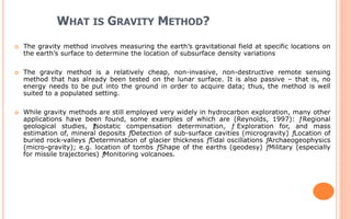
GLG 831 GEOPHYSICS_GRAVITY METHOD...pptx

MODULE 1: GRAVITY METHOD
Ugwuada ThankGod Chinemerem
Presenter
GLG 831: GRAVITY AND MAGNETIC METHOD

WHAT IS GRAVITY METHOD?
 The gravity method involves measuring the earth’s gravitational field at specific locations on
the earth’s surface to determine the location of subsurface density variations
 The gravity method is a relatively cheap, non-invasive, non-destructive remote sensing
method that has already been tested on the lunar surface. It is also passive – that is, no
energy needs to be put into the ground in order to acquire data; thus, the method is well
suited to a populated setting.
 While gravity methods are still employed very widely in hydrocarbon exploration, many other
applications have been found, some examples of which are (Reynolds, 1997): ƒRegional
geological studies, ƒ
Isostatic compensation determination, ƒ Exploration for, and mass
estimation of, mineral deposits ƒ
Detection of sub-surface cavities (microgravity) ƒ
Location of
buried rock-valleys ƒ
Determination of glacier thickness ƒ
Tidal oscillations ƒ
Archaeogeophysics
(micro-gravity); e.g. location of tombs ƒShape of the earths (geodesy) ƒMilitary (especially
for missile trajectories) ƒ
Monitoring volcanoes.

INERTIAL AND GRAVITATIONAL MASS
There are two kinds of mass define by the m in their equations:
inertial (F=ma) and gravitational ( g=Gm/r2 ).
Should the two mass (m) be the same ?
But we now know that the two mass kinds are the same (relativity).
A detail is that force, momentum, and velocity are vectors in 3-space.
Inertial mass is define as m = F/a. This mass can be measured by applying a
force to an object and measuring its acceleration. This mass is thus a measure
of the inertia of an object. And, inertia is the FACT that masses remain at rest or
in straight-line constant velocity motion UNLESS acted upon by an unbalanced
force. And a force is defined as a change in an object velocity vector
(momentum: p=m.v).
Gravitational mass is defined as m = g(r).r2 / G. This mass can be measured
by measuring the gravity field at a distance r and knowing the value of big-G.
This mass is thus a measure of the gravitational acceleration field made by ALL
objects (mass).
3

4
Gravitational force law and Inertial force Law
1 2
2 1
1 2
2 2
1
1 2 1
2 2
2
2 1 2
2 2
( ) ( )
( ) ( )
( ) ( )
on
on
m m
m m
m m m
F r G Newtons kg
r s
m m
g r G F m g
r s
m m
g r G F m g
r s

  
  
•The two Forces (F) is the magnitude of the force applied by
mass 1 on mass 2 AND the force of mass 2 on mass 1.
•The direction of the two force is equal and opposite in
direction.
•This unbalanced force will cause each mass to accelerate in
inverse proportion to its mass: a = F/m.
•The little mass accelerates much more than the big mass,
but the forces magnitudes are the same!
So when I drop a ball, the ball accelerates
down at 9.8 m/s.2…yes.
And, the earth accelerates upwards towards
the balls mass….yes.
Why don’t we notice the earth’s upward
acceleration?

BASIC THEORY
 The basis on which the gravity method depends is encapsulated in two laws
derived by Newton, namely his Universal Law of gravitation, and his Second
Law of Motion.
 The Universal Law of gravitation, states every particle in universe attracts
every other particle with a force that is directly proportional to the product of
their masses and inversely proportional to the square of the distance between
them
(Equation 1)
 where the gravitational constant, G = 6.67 x 10-11 Nm2 kg-2
 NB: Force of gravity is measured in Newton's (N)
E M
Fe
Fm
FG =
M1 . m2
r 2
G

BASIC THEORY
• Newton’s law of motion states that a force (F) is equal to mass (m) times
acceleration (Equation 2). If the acceleration is in a vertical direction, then it is due
to gravity (g).
(Equation 2)
Force (F) = mass (m) × acceleration (g)
F = M X G
• Equations 1 and 2 can be combined to obtain another simple relationship:
• This shows that the magnitude of acceleration due to gravity on Earth (g) is
directly proportional to the mass (M) of the Earth and inversely proportional to the
square of the Earth’s radius (R).

DERIVATION OF THE GRAVITATIONAL CONSTANT (G)

• The normal value of g at the Earth’s surface is 980 cm/s2 . However, In
honour of Galileo, the c.g.s. unit of acceleration due to gravity (1 cm/s2 ) is
Gal.
•Furthermore, Modern gravity meters (gravimeters) can measure extremely
small variations in acceleration due to gravity, typically 1 part in 109 . The
sensitivity of modern instruments is about ten parts per million. Such small
numbers have resulted in sub-units being used such as the:
milliGal (1 mGal = 10-3 Gal);
microGal (1 μGal = 10-6 Gal); and
1 gravity unit = 1 g.u. =0.1 mGal [10 gu =1 mGal]

GRAVITY TOOLS/ EQUIPMENT
• There are two kinds of gravity meters. An absolute gravimeter which
measures the actual value of g by measuring the speed of a falling mass using a
laser beam, and can reach precisions of 0.01to 0.001 mGal (miliGals, or 1/1000
Gal).
• A second type of gravity meter is the Relative gravimeter which measures
relative changes in g between two locations. This instrument uses a mass on the
end of a spring that stretches where g is stronger. This kind of a meter can
measure g with a precision of 0.01 mGal in about 5 minutes.
•A relative gravity measurement is also made at the nearest absolute gravity
station, one of a network of worldwide gravity base stations and are thereby tied
to the absolute gravity network.
• The common gravimeters on the market are the Worden gravimeter, the
Scintrex and the La Coste Romberg gravimeter.

MEASURING GRAVITY WITH A GRAVIMETER
11
In a simple sense, a gravimeter measures gravitational variations by using Hooke’s Law of elasticity that states
that the force required to extend a spring is
F = k . dx where k is the spring stiffness and dx is a small displacement of the spring from equilibrium
position.
So, as the force of gravity applied to the mass (m) varies as one moves the gravimeer around a survey, the
mass position changes (dx) proportional to the spring stiffness (k).
Note: we are only measuring relative variations, not the absolute value of gravity.

HOOK’S LAW EXPLAINING THE PRINCIPLE OF THE
GRAVIMETER
 Stating parameters
F = mg, (Eqn 1)
And, F ~ e (Eqn 2)
Removing the proportionality sign and adding equality, then
introducing a constant, k. where have that.
F = K (L2 – L1) (Eqn 3)
Substituting (Eqn 1) into (Eqn 3), we have that:
Mg = K (L2 – L1) (Eqn 4)
Making (g) the subject of Eqn 4; g = K (L2 – L1) / m; g = k/m (L2/L1 -
1)

MEASURING GRAVITY REDUX
13
In practice, measuring gravitational variations
requires a very precise instrument that costs
>40,000 dollars.
1. The temperature must be keep stable to
<1° C using thermistors and heaters.
2. The beam must be very accurately
engineered so that the change in force
associated with the change in the spring-
beam angle is compensated.
A modern instrument can measure
changes in gravity to one part in a million
(i.e., 1 inch height variation!).

GRAVITY TOOLS/ EQUIPMENT CONT.
A B
(A) Image of an Absolute Gravimeter (B) Image of the La coste Romberg gravimeter, which is the
most popularly used Relative gravimeter

CALCULATING GRAVITY FOR GENERAL SHAPES
15
Problem: how to calculate gravity field between a point mass (m2) and a general
mass distribution on left side (i.e., earth, asteroid)?
Easy, divide the general shape into little squares (2-d) or cubes (3-d) and label them
(I and J) and then add up the vector forces applied by all the little cubes on mass
m2.

CALCULATING GRAVITY OF PERFECT SPHERES
16
When an object’s geometry can be approximated
as a sphere, we integrate (add-up) the sphere’s
gravity using spherical shells that extend over a
small radial distance.
In doing this integration, we find that the
symmetry of the sphere makes the sphere’s
gravity field to be the same as if ALL the mass was
concentrated at the center of the sphere!!
One caveat: the ability to treat a sphere’s mass
distribution as a point is true ONLY IF the ms mass is
outside the radius of the sphere.
This theorem found by Newton greatly simplifies the
mathematics by treating the Me spherical mass as a
point!
Easy to apply to solar system as all the masses are near
spherical. On the other hand, it is the Earth’s non-
spherical ellipsoidal shape that makes the moon recede
from the earth about 3.8 cm/yr and the earths rotation to
slow by 0.002 s a day.

CALCULATE GRAVITY DIRECTLY ABOVE A SPHERICAL MASS ANOMALY
17
5 2
1 10 /
mGal m s


The gravity signal directly above a sphere whose center is at
100 m depth and has a density contrast of 0.3 Mg/m3 is
+1.048e-6 m/s2 .
But, let us convert that answer to Mgal units.
+1.048e-6 m/s2 . 1 Mgal/(10-5 m/s2 ) = 0.1 Mgal
That is an large enough signal to be measured with a
decent gravimeter.

DENSITIES OF ROCKS AND LIQUIDS
18
Notice we are not using the MKS mass units of
kilo-grams (kg) for density.
Mass is being reckoned in mega-grams which is
a thousand (103 ) grams.
Note that in general the substances density
increase as follows: liquids, unconsolidated
sediments, sediments, igneous/metamorphic
rocks, minerals/ores.
Density is defined by the Greek letter rho as:
mass
volume
 

DATA ACQUISITION
• Gravity data acquisition is a relatively simple task that can be performed by one
person. However. Two people are usually necessary to determine the location of
the gravity stations.
• Surveys are conducted by taking gravity readings at regular intervals along a
traverse that crosses the expected location of the target
•To make accurate measurements, the instrument must be level (aligned with the
vector of the Earth’s gravity field), in a place quiet enough to avoid vibrations
(trucks rumbling by and earthquakes are a problem!), and given sufficient time to
be in thermal and mechanical equilibrium (avoiding sharp changes in
temperature that effect the instrument’s metal parts, etc.).
• However, in order to take into account the expected drift of the instrument, one
station must be located and has to be reoccupied every half to 1 hr or so to
obtain the natural drift of the instrument.

DATA ACQUISITION
• These repeated readings are performed because even the most stable gravity
meter will have their readings drift with time due to elastic creep within the
meters springs
•The Instrument drift is usually linear and less than 0.01 mGal/hour
• From the drift curve, a base reading corresponding to the time a particular
gravity station was measured is obtained by subtracting the base reading from
the station reading.

CALCULATING GRAVITY AT DIFFERENT POINTS ON SURFACE
22
To calculate the gravity effect of the
irregular body above at point P1 , the body
is divided into small squares (parcels) and
the many gravity vectors from all the
parcels are added up to get the total
gravity. Do the same analysis to get the
gravity at the other points.
An important detail. The gravity field is a vector quantity
(has magnitude and direction). When measuring the
gravity of the above situation, both the ‘pull of rest of
Earth’ and the ‘total pull of excess mass of body’ are
measured. Note that with respect to point P, the Earth and
the ‘body’ pull at different directions. When can ignore this
detail, because the Earth’s pull is so much greater, and just
assume we are measuring the ‘vertical component of Fb
‘ .

DATA PROCESSING AND CORRECTION/REDUCTION
• Gravimeters do not give direct measurements of gravity. Rather, a meter
reading is taken which is then multiplied by an instrumental calibration factor to
produce a value of observed gravity (gobs). The correction process is known as
gravity data reduction or reduction to the geoid.
• However, to successfully interpret gravity data, one must remove all known
gravitational effects not related to the subsurface density changes.
• Each reading has to be corrected for elevation, the influence of tides, latitude
and, if significant local topography exists, a topographic correction.
• Which brings us to the various kinds of Gravity data correction:

DATA PROCESSING AND CORRECTION/REDUCTION
LATITUDE CORRECTION
DRIFT CORRECTION
BOUGUER CORRECTION
TIDAL CORRECTION

TIDAL CORRECTION
• The Tidal correction accounts for the gravity effect of sun,
moon and large planets.
• Just as the water in the oceans responds to gravitational
pull of the Moon, and to a lesser extent of the Sun, so too
does the solid earth. ET give rise to a change in gravity of up
to three g.u. with a minimum period of about 12 hours.
•However, Repeated measurements at the same stations
permit estimation of the necessary correction for tidal effects
over short intervals, in addition to determination of the
instrumental drift for a gravimeter.

LATITUDE CORRECTION
• Correction subtracted from gobs (Gravity Observed) that
accounts for Earth's elliptical shape and rotation. The gravity
value that would be observed if Earth were a perfect (no
geologic or topographic complexities), rotating ellipsoid is
referred to as the normal gravity
• The earth is not a sphere, but a flattened spheroid with an
equatorial radius of 6,378km and a poplar radius of 6,356km
(21km different). Thus, the gravity is LESS at the equator
because it is FARTHER AWAY from the earth’s center of
mass.

LATITUDE CORRECTION CONT.
• The earth is a non-inertial reference frame because it is a
rotating body that spins once per day. At the equation any
object has a rotational velocity of 456 m/s. where as at the
poles the rotational velocity is zero! Physics requires that a
rotational reference frame has non-intertial forces such as
the outward such as the outward directed centrifugal force.
This outward force is in opposite direction to gravity force at
equator, thus reduce gravity force at equator as compared to
poles
• In other words gravity varies from 9.78 m/s2 at the equator
to 9.83 m/s

LATITUDINAL GRAVITY CORRECTIONS
28
2 2 3 6
1 2 3 1 2 3
( ) (1 sin sin 2 ), 9.78031, 5.3024 , 5.900 .
g e e
        
 
     
Gravity varies from 9.78 m/s2 at the equator (lat=0°) to 9.83 m/s2 at the poles (lat: north = +90°; south = -90°). This
is a huge change: a 0.052 m/s2 variation equals 5200 mgals! This is much larger than other gravitational effects.
The gravity varies with latitude for two reasons:
• The Earth is not a sphere, but a flattened spheroid with an equatorial radius of 6,378 km and a polar radius of
6,356 km (21 km different). Thus, the gravity is LESS at the equator because it is FARTHER AWAY from the
Earth’s center of mass.
• The Earth is a non-inertial reference frame because it is a rotating body that spins once per day. At the equator
any object has a rotational velocity of 465 m/s, whereas at the poles the rotational velocity is zero! Physics
requires that a rotational reference frame has non-inertial (fictitious) forces such as the outward directed
centrifugal force. The centrifugal force is the force that any mass rotating with the planet ‘feels’ in response to
the centripetal force that the planet’s gravity field provides to continually curve an object’s path on the earth
intoa circular path. Recall Newton’s first law says that all masses go in a straight line in a INTERTIAL reference
frame unless acted on by an unbalanced force (it is gravity that provides the unbalanced force as a centripetal
acceleration).
The International gravity formula that describes latitudinal (Ѳ) gravity variations in m/s2 units is:
An approximate latitudinal equation when
survey is small.

DRIFT CORRECTION
• This correction is intended to remove the changes caused by the
instrument itself. If the gravimeter would be at one place and take
periodical readings, the readings would not be the same.
• These are partly due to the creep of the measuring system of the
gravimeter, but partly also from the real variations — tidal
distortion of the solid Earth, changes of the ground water level,
etc.
• The drift is usually estimated from repeated readings on the base
station. The measured data are then interpolated, e.g. by a third
order polynomial, and a corrections for profile readings are found.

BOUGUER CORRECTION
• The Bouguer correction is a first-order correction to account for the excess
mass underlying observation points located at elevations higher than the
elevation datum (sea level or the geoid). Conversely, it accounts for a mass
deficiency at observation points located below the elevation datum. The form of
the Bouguer gravity anomaly, gb, is given by.
• where r is the average density of the rocks underlying the survey area.
•Terrain corrected bouguer gravity (gt ) - The terrain correction accounts for
variations in the observed gravitational acceleration caused by variations in
topography near each observation point. Because of the assumptions made
during the Bouguer Slab correction, the terrain correction is positive regardless of
whether the local topography consists of a mountain or a valley. The form of the
Terrain corrected, Bouguer gravity anomaly, gt , is given by:

BOUGUER CORRECTION CONT.
• where TC is the value of the computed terrain correction.

TOPOGRAPHIC CORRECTIONS
32
The free-air correction using sea-level as a datum is 0.3086 Mgal/m. If gravity is measured above one’s
datum the effect is added and if gravity is measured below one’s datum the effect is subtracted. Why did
we define the sign of the correction this way?
The Bouguer correction uses the infinite sheet gravity equation to approximate the gravity of the material
above or below sea-level. The relevant quantities are the thickness of the sheet (h), the sheets density,
and the sign of h (positive if above base station negative if below base station).
Combining the free-air and Bouguer gravity
effects gives Eqn. 8.11

ALL TOGETHER: ADDING OR SUBTRACTING THE GRAVITY
CORRECTIONS
33
It is very important to keep physical track of the sign of the corrections; if you do not, you will get the
wrong answer. Remember, we are correcting the measured gravity data to remove unwanted effects.
The free-air effect is added if you are above sea-level and is subtracted if you are below sea-level.
The Bouguer effect is subtracted if you are above sea-level (+h) and added if you are below sea-level (-h).
Total Bouguer correction : Bouguer = observed – latitude +/- free-air +/- Bouguer
Total correct to Free-air: Free-air = observed – latitude +/- free-air
The sign of the free-air and Bouguer correction depends on whether the measurements was made above
or below ones datum.

DATA INTERPRETATION
• In common practice, gravity and other potential field data are acquired along a
series of parallel profiles. Thus the data can be viewed and interpreted either as
profiles or, in two directions, as a map of isoanomaly contours.
• While machine contouring is very common for large data-sets, Presentation
and analysis of data in profile form has some specific advantages.
• Furthermore, Profile interpretation is theoretically valid if the anomaly sources
strike perpendicular to the profile and are two-dimensional (2-D).
• The objective of gravity interpretation is to deduce from the various
characteristics (in particular the amplitude, shape, and sharpness) of the
anomaly the location and form of the subsurface structure which produces the
gravity disturb.
•For this purpose, the data have to be analyzed by suitable interpretation
techniques.

DATA INTERPRETATION: AMBIGUITY IN GRAVITY
INTERPRETATION
• There are two characteristics of the gravity field which make a unique
interpretation almost impossible. The first is that the measured value of g, and,
therefore, also the reduced anomaly, AgB, at any station represents the
superimposed effect of many mass distributions at various depths.
• The second, and more serious, difficulty in gravity interpretation is that of
determining the 'source' from the 'effect', which is the inverse problem of the
potential. However, For a given distribution of gravity anomaly on (or above) the
earth's surface, an infinite number of mass distributions can be found which would
produce the same anomaly

DATA INTERPRETATION: AMBIGUITY IN GRAVITY
INTERPRETATION
The Figure shows how a given gravity anomaly could be explained by any of the
alternative mass distributions (cases 1-3) showing a fixed density contrast, Ap, with
respect to the surrounding material. The figure also illustrates another type of
ambiguity arising from lack of information about the density contrast. If we assume
that the anomaly results from a body of spherical shape, various interpretations of
the size (i.e., volume, V) of the sphere are possible, although the anomalous mass
(product VAp) can be determined uniquely. This type of ambiguity cannot be
resolved unless Ap is reliably known.

DATA INTERPRETATION: ISOLATION OF ANOMALIES
• Regional anomaly represents large-scale variations in the gravity or magnetic
field caused by broad geological features, while, Residual anomaly represents
local or more specific changes in the subsurface, such as the presence of mineral
deposits, fault lines, or other geological structures.
• However it is important to note that The separation of the residual anomaly of a
potential field distribution is a critical problem which controls the accuracy of the
interpretation process
Image showing the residual and regional anomaly on a Graphical method of separation of
the regional and local anomalies

DATA INTERPRETATION: ISOLATION OF ANOMALIES
• In a gravity map of a small area, the regional trend may appear as a uniform
variation represented by nearly parallel, evenly spaced contours. A local anomaly,
which ordinarily would be indicated by closed contours, appears as a 'nose' on the
regional anomaly field.
• The anomaly separation procedure may consist of the removal of the regional
effect by either of two methods: (1) graphical smoothing, either on the contour
map or on profiles; (2) an analytical process applied to an array of values,
usually on a regular grid.
• In the graphical approach, the value of the visually smoothed regional field on the
profile can be subtracted from the original Bouguer anomaly at the point to give the
'residual' anomaly
•The analytical approach is based on suitably averaging the anomaly data at equal
distance around a station to obtain the regional (smoothed) value and subtracting
this from the Bouguer value of the station to get the residual.

GRAVITY ANOMALIES OF A SPHERE A CYLINDER
39
The y-axis is the gravity anomaly (mgal) and the x-axis is distance from the center of the
sphere/cylinder (m). These graphs are cross-section through these 3-d objects. The cylinder extends to
+/- infinite in and out of the page. This is why, for the same depth object and mass anomaly, the
cylinder and sphere anomalies are different.
Important: Note that the peak amplitude reduces and the anomalies ‘half-width’ widens as the
anomaly is placed deeper. This is just a consequence of gravity being an ‘inverse square law’.

GRAVITY ANOMALIES OF DIPPING NARROW MASS SHEETS
40
Note three gravity effects:
As the depth to the top of the
anomalies increases the peak
amplitude of the anomaly
decreases.
As the sheet anomaly dips to one side,
the anomaly’s peak value moves to
that side.
As the sheet anomaly dips to one side,
the anomaly has a long-tail on that
side, and a short tail on the other
side.
From these effects, we can determine
the dip of the sheet anomaly.
What is the sign of the mass anomaly?

GRAVITY OF INFINITE HORIZONTAL SHEET
41
The gravity anomaly of an infinite horizontal sheet at depth d and width t provides an interesting
rendezvous with infinity. First, note that the sheet depth d is NOT in the equation. Second, even though
the mass sheet anomaly extends to infinity, the gravity is finite because of the ‘inverse square law’. Third,
the gravity effect is the same everywhere as demonstrated above where it can be seen that the gravity at
points P1 and P2 are the same. Thus, an infinite sheet anomaly makes the gravity everywhere change by
the same values as given by Eqn. 8.6. Therefore, one cannot detect an infinite mass sheet. But, we will use
this concept to calculate the Bouguer gravity correction.
Bouguer gravity reduction equation
Why is gravity not infinite for a 2-d infinite sheet?

GRAVITY EFFECTS OF HALF-SHEETS
42
Note two effects:
1. The deeper sheet has a smaller
peak anomaly.
2. The deeper sheet has a wider
anomaly half-width.
What happens if the mass anomaly
sign is reversed ?
Figure (a) shows a stratigraphic section with different layer
densities that has be offset by a vertical fault.
Figure (b) shows the layer densities changed into density
contrasts so that we can easily calculate the total gravity
anomaly associated with the variable vertical distribution of
density. From this the relative motion of the fault can be
determined. What is it ?

DATA INTERPRETATION: ENHANCEMENT OF ANOMALIES
• In a gravity map of a small area, the regional trend may appear as a uniform
variation represented by nearly parallel, evenly spaced contours. A local anomaly,
which ordinarily would be indicated by closed contours, appears as a 'nose' on the
regional anomaly field.
• The anomaly separation procedure may consist of the removal of the regional
effect by either of two methods: (1) graphical smoothing, either on the contour
map or on profiles; (2) an analytical process applied to an array of values,
usually on a regular grid.
• In the graphical approach, the value of the visually smoothed regional field on the
profile can be subtracted from the original Bouguer anomaly at the point to give the
'residual' anomaly
•The analytical approach is based on suitably averaging the anomaly data at equal
distance around a station to obtain the regional (smoothed) value and subtracting
this from the Bouguer value of the station to get the residual.

ESTIMATES OF DEPTH AND ANOMALOUS MASS
• In general the sharpness of an anomaly is an index of the depth of the causative
source.
• If some simplified shape for the causative body can be postulated, simple depth
rules in terms of 'half-width' or some other measure of the anomaly gradient can
provide unambiguous estimates of depth.
• It is also good to note that There are no simple depth rules for finite bodies of non-
spherical shape. In addition, for finite horizontal and vertical cylinders there are no
analytical formulas (expressions in closed form) for calculating their gravity effects.
• Also The magnitude of a gravity anomaly is a direct measure of mass, and the
total anomalous mass can be uniquely determined without any assumption
whatsoever about the shape, density, and depth of the anomalous body. The basis
of the calculation is a Gaussian surface integration of the residual anomaly (i.e.,
Bouguer minus regional) over the area of measurement. The formula for the total
anomalous mass is

• Where Ag is the mean anomaly (g.u.) within a small area element AS (m2 ) and 2
denotes the summation of the product AgXAS over the whole area of perceptible
anomalies.

Horizontal variation in gravity due to a sphere and a horizontal cylinder, both
of radius R and density contrast (Ap=p2-p1). The maximum anomaly occurs at
x=0 and falls to its half-value at x=x1/o

Form of the gravity anomaly across a vertical fault. Over the fault trace the
total change in gravity (Agmax) falls to its half-value. The horizontal distance,
xp over which the anomaly changes from 0.5Agmax to 0.25Agmax is a
measure of the depth, z

DEPTH/HALF-WIDTH RULES FOR
DIFFERENT GEOMETRY MASS ANOMALIES
48
Note systematic variations
between the depth to bodies
and the half-width of the gravity
profiles.
(a) Sphere.
(b) Horizontal cylinder.
(c) Steeply dipping sheet.
For the Irregular body, the peak
anomaly and maximum
slope value are required.

HANDS-ON GRAVITY DATA REDUCTION
(PRACTICAL EXAMPLE)
• The table shows data collected along a north–south gravity profile. Distances
are measured from the south end of the profile, whose latitude is 51°12’ 24’’ N.
The calibration constant Gravity Surveying 151 of the Worden gravimeter used
on the survey is 3.792gu per dial unit. Before, during and after the survey,
readings (marked BS) were taken at a base station where the value of gravity is
9811442.2gu. This was done in order to monitor instrumental drift and to allow
the absolute value of gravity to be determined at each observation point.
•Use a density of 2.70Mgm-3 (2.70 g/cc) for the Bouguer correction

STATION TIME DIST. (m) ELEV.(m) READING
BS 805 2935.2
1 835 0 84.26 2946.3
2 844 20 86.85 2941
3 855 40 89.43 2935.7
4 903 60 93.08 2930.4
1 918 2946.5
BS 940 2934.7
1 1009 2946.3
5 1024 80 100.37 2926.6
6 1033 100 100.91 2927.9
7 1044 120 103.22 2920
8 1053 140 107.35 2915.1
1 1111 2911.5
BS 1145 2907.2
1 1214 2904
9 1232 160 110.1 2946.5
10 1242 180 114.89 2935.2
11 1300 200 118.96 2946.2
1 1315 2946.3
BS 1350 2935.5
Hence:
Calibration factor = 3.792 g.u = 0.3792 mgal;
Absolute gravity at Base station = 9811442.2gu = 981144.22mgal

PERFORMING DRIFT CORRECTIONS.
BS GRAVITY
READING, 2935.5
2933.5
2934
2934.5
2935
2935.5
2936
805 940 1145 1350
Gravity
Reading
Gravity Drift Curve

BOUGUER ANOMALY CURVE.
-25.00000
-24.00000
-23.00000
-22.00000
-21.00000
-20.00000
-19.00000
-18.00000
-17.00000
-16.00000
-15.00000
0 50 100 150 200 250
Bouguer
Anomaly
Axis Title
Station Distance meters

CALCULATING DEPTH TO SUBSURFACE BODY
-25.00000
-24.00000
-23.00000
-22.00000
-21.00000
-20.00000
-19.00000
-18.00000
-17.00000
-16.00000
-15.00000
0 50 100 150 200 250
Bouguer
Anomaly
Axis Title
Station Distance meters
X
Y

CHALLENGES AND LIMITATION OF THE GRAVITY METHOD
Interpretation Complexity: Interpreting gravity data requires a good
understanding of geology. Different geological structures can produce
similar gravity anomalies, making it challenging to differentiate between
them without additional information.
Depth Ambiguity: Gravity data primarily reflects variations in density
beneath the Earth's surface. However, it doesn't provide a direct
measure of depth. Ambiguity in depth interpretation can arise, especially
when dealing with multiple subsurface layers.
Environmental Interference: Local variations in Earth's density due to
factors such as changes in topography, vegetation, and cultural features
(buildings, roads) can interfere with gravity measurements. Correcting for
these environmental effects can be complex.

CHALLENGES AND LIMITATION OF THE GRAVITY METHOD
CONT.
Cost and Logistics: Conducting gravity surveys can be expensive,
especially in remote or challenging terrains. The logistics involved in
deploying equipment and collecting data across large areas can pose
practical challenges.
Weather Sensitivity: Gravity measurements can be affected by weather
conditions, such as atmospheric pressure changes. Corrections for these
variations are necessary for accurate results.

LEARNING OUTCOME
 I am able to explain the working principles behind the gravimeter
using hook’s law of elastic materials
 I am bale to apply all the various gravity data reduction techniques
into a known raw gravity data.
 I am able to determine using the appropriate formula the depth to a
subsurface body
 I have understood and able to interpret a gravity anomaly
 I am able to subtract a residual anomaly out of a regional anomaly
 I am able to state some of the challenges and limitation of the gravity
method
 I am able to state the most important application for the gravity
method

 I am able to explain the principles of gravity using the 2 laws of
Newton
LEARNING OUTCOME

SIMPLE PENDULUM PRACTICAL ASSIGNMENT
Simple pendulum experiment done in 2 various locations with the aim to determine the absolute
gravity in the location
Mass of the pendulum (m) = 35g
Length of thread (L) = 0.30m
No of Oscillation (Os) = 20
Time = t
Period (T) = t/Os
g (Gravity) = 4π2L/T2
Π = 3.142
First
Experiment
Second
Experiment
Third
experiment
Average
Time 21.76 21.65 21.38 21.60
Latitude 6 50’ 40’’ N
Longitude 7 22’ 53.53’’ S
Elevation 468m
LOCATION 1
First
Experiment
Second
Experiment
Third
experiment
Average
Time 21.80 21.88 21.90 21.86
Longitude 6 52’ 40’’ N
Latitude 7 24’ 53.53’’ S
LOCATION 2

SIMPLE PENDULUM CALCULATIONS
• Location 1
T = 21.60/20 = 1.08s
g = 4 x (3.142)^2 x 0.30/ (1.08)^2
g = 11.85/1.1664
g = 10.16 m/s^2
• Location 2
T = 21.86/20 = 1.093s
g = 4 x (3.142)^2 x 0.30/ (1.093)^2
g = 11.85/1.195
g = 9.91 m/s^2

INTERNATIONAL GRAVITY FOMULAR
Formula: g = 9.780327 x (1 +0.0053024 x sin^2 (lat) – 0.0000058 x sin^2 (2 x lat)) – 0.000003086 X
elevation
• Location 1
Lat (Radians) = 0.119460
Substitute the value of the ,lat to the formula;
9.780327 x (1 +0.0053024 x sin^2 (0.119460) – 0.0000058 x sin^2 (2 x 0.119460)) – 0.000003086 X
468
g = 9.762 m/s^2
• Location 2
Lat (Radians) = 0.11987
Substitute the value of the ,lat to the formula;
9.780327 x (1 +0.0053024 x sin^2 (0.11987) – 0.0000058 x sin^2 (2 x 0.11987)) – 0.000003086 X 437
g = 9.763 m/s^2

RESULTS AND CORRECTION OF GRAVITY DATA GOTTEN FROM 42˚ N
QUESTIONS 1 (a)
Meter reading at CLS lobby (base) mGal = 380.10
Meter Conversion Factor, 1 meter unit is (mGal) = 0.09520
Gravity at base station (CLS lobby) (mGal) = 980680.00
Density for Bouguer Correction (g/cc) = 2.67

313
313.5
314
314.5
315
315.5
0 100 200 300 400 500 600 700
Bouguer Anomaly mgal
Bouguer Anomaly mgal
GRAVITY ANOMALY GRAPH

QUESTION 1 (c)
The gravity anomaly associated with a shear zone is not symmetric, it suggests that the mass
distribution causing the anomaly is not uniform or symmetrical. The lack of symmetry in the
gravity anomaly implies variations in the density or thickness of the material within the shear
zone or its surroundings. This could be indicative of a more complex geological structure like
Adjacent Geological Features, Multiple Shear Zones or Faults, etc.

ANSWER: To find the maximum gravity anomaly, we need to analyze the behavior of this function.
The maximum will occur where the derivative with respect to x equals zero.
Analyzing the terms inside the brackets, as x approaches ℎ, the second term dominates due to the
smaller value in the denominator. Thus, the gravity anomaly will be maximized near x=h.
In words, we expect to find the maximum gravity anomaly due to this pair of anomalous masses
near the horizontal location x=h, which is the horizontal distance between the centers of the two
cylinders.
QUESTION 2

SOLUTION ASSIGNMENT 2
 Parameters:
 Gravitational constant (G) = 6.6743 × 10^-11 m^3 kg^-1 s^-2
 Density of surrounding rock (ρ_rock) = 2.4 × 10^3 kg/m^3
 Density of lava tube (ρ_lava) = 3.0 × 10^3 kg/m^3
 Radius of lava tube (r) = 20 m
 Depth to center of lava tube (h) = 40 m

 Gravitational Attraction of Rock:
g_rock = (G . ρ_rock . π . h . r^2) / (2 . ρ_rock . π . r^2 . h) = G .
ρ_rock / 2
 Gravitational Attraction of Lava Tube:
g_lava = (G . ρ_lava . π . h . r^2) / (2 . ρ_lava . π . r^2 . h) = G .
ρ_lava / 2
 Change in Observed Gravity (Δg):
Δg = g_lava - g_rock = (G . ρ_lava / 2) - (G . ρ_rock / 2) = G .
(ρ_lava - ρ_rock) / 2
Δg ≈ 1.889 × 10^-7 m/s² (or 18.89 micro gals)

Free-air Gravity (g_free_air):
NB: As the free-air correction accounts for the mass deficit above the station due to its elevation, it
won't be affected by the presence of the lava tube. Therefore, g_free_air remains the same as
g_rock:
g_free_air ≈ 3.337 × 10^-11 m/s² (or 0.033 microgals)
Bouguer Anomaly (Δg_Bouguer):
Δg_Bouguer = Δg - g_free_air = 1.889 × 10^-7 m/s² - 3.337 × 10^-11 m/s² ≈ 1.889 × 10^-7 m/s² (or
18.89 microgals)
Interpretation
The presence of the denser lava tube creates a positive change in observed gravity (Δg) of
approximately 18.89 microgals compared to the old site. This indicates an attraction towards the
lava tube.
Since the free-air correction is independent of subsurface features, the free-air gravity remains
practically unchanged at the new site.
The Bouguer anomaly also shows a positive value of around 18.89 microgals, confirming the
presence of a denser mass (lava tube) below the new station.

GLG 831 GEOPHYSICS_GRAVITY METHOD...pptx

More Related Content

What's hot

Similar to GLG 831 GEOPHYSICS_GRAVITY METHOD...pptx

Recently uploaded

GLG 831 GEOPHYSICS_GRAVITY METHOD...pptx