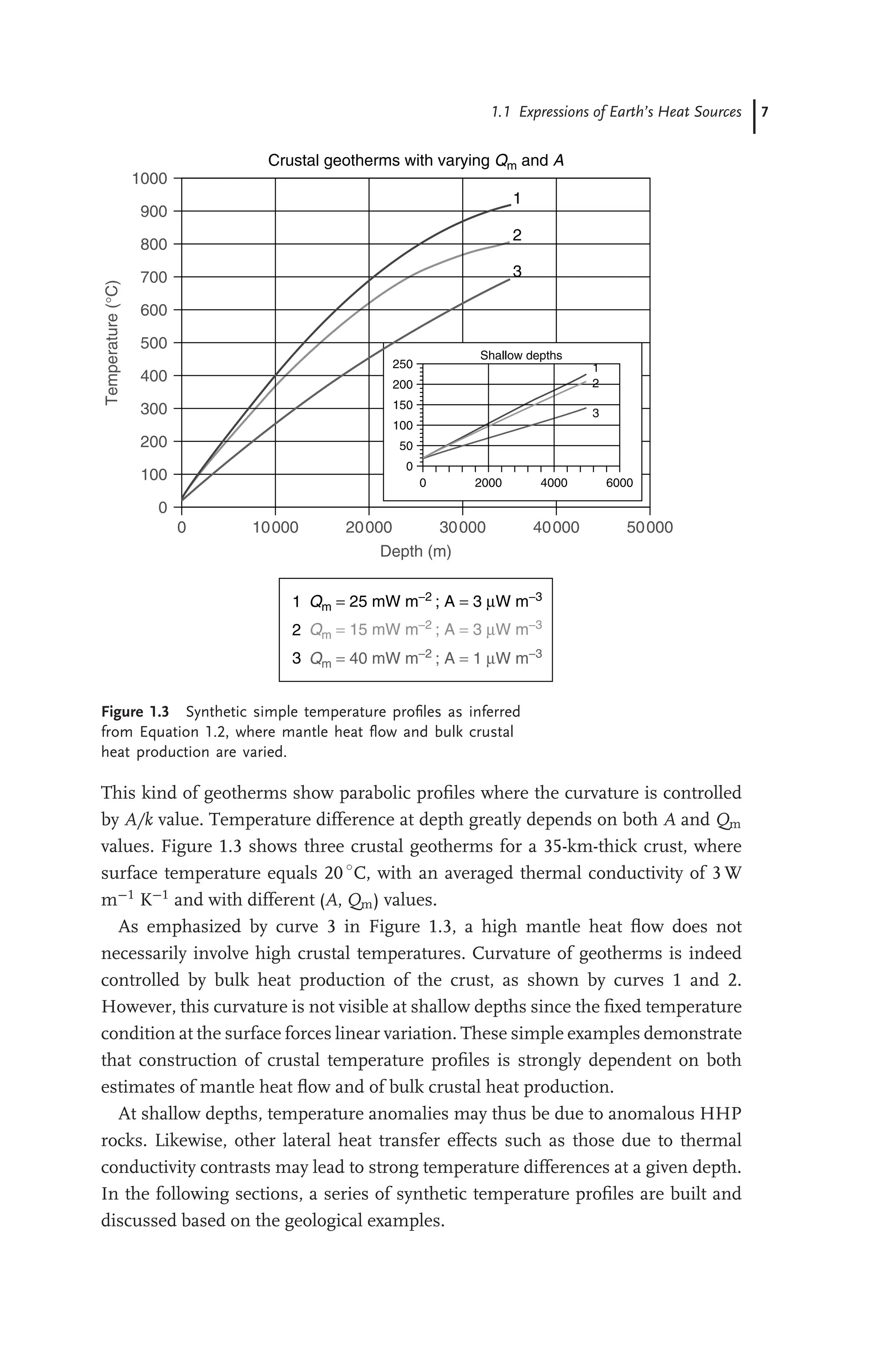
Geothermal Energy Systems Exploration Development And Utilization 1st Edition Ernst Huenges
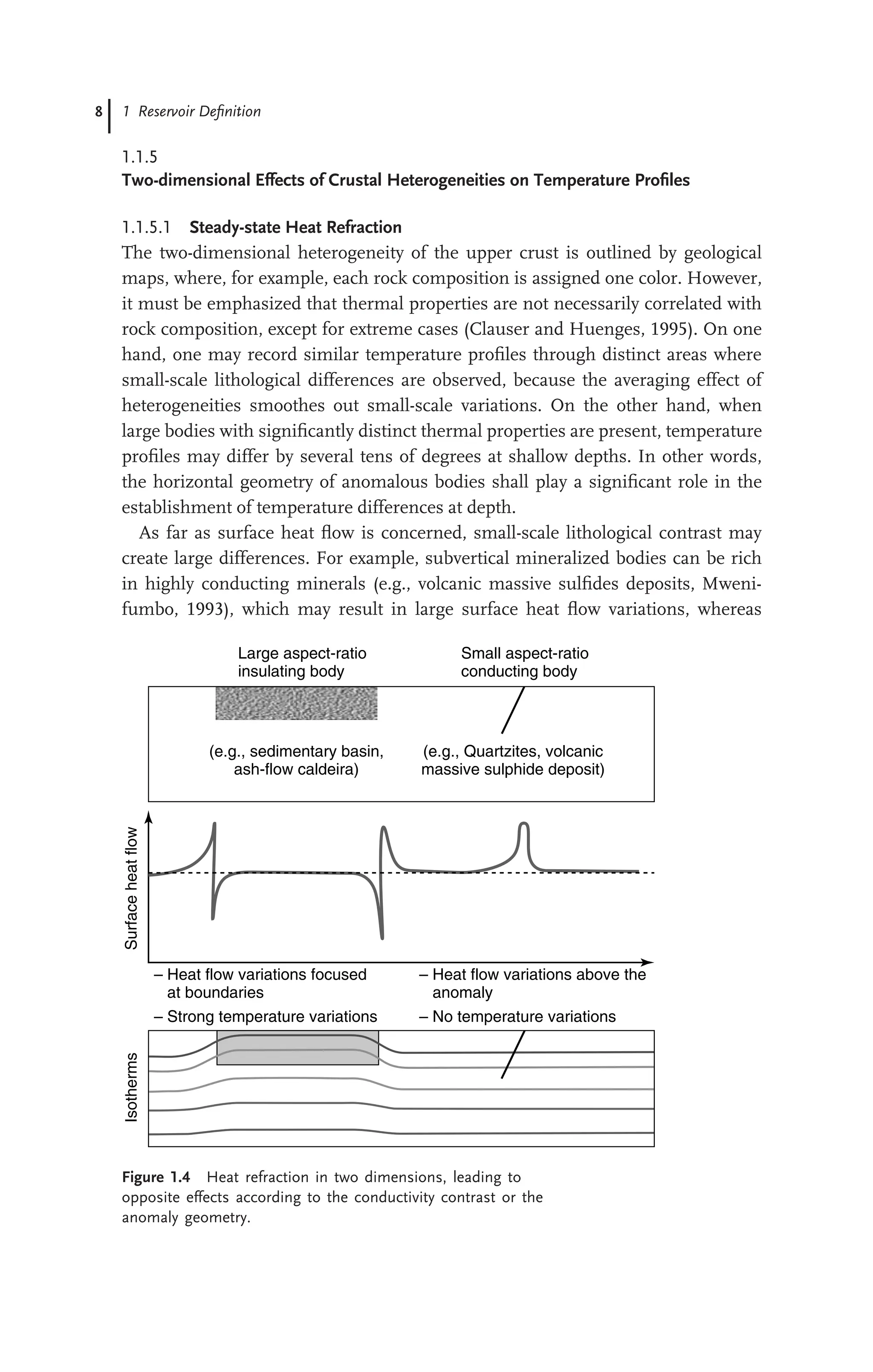
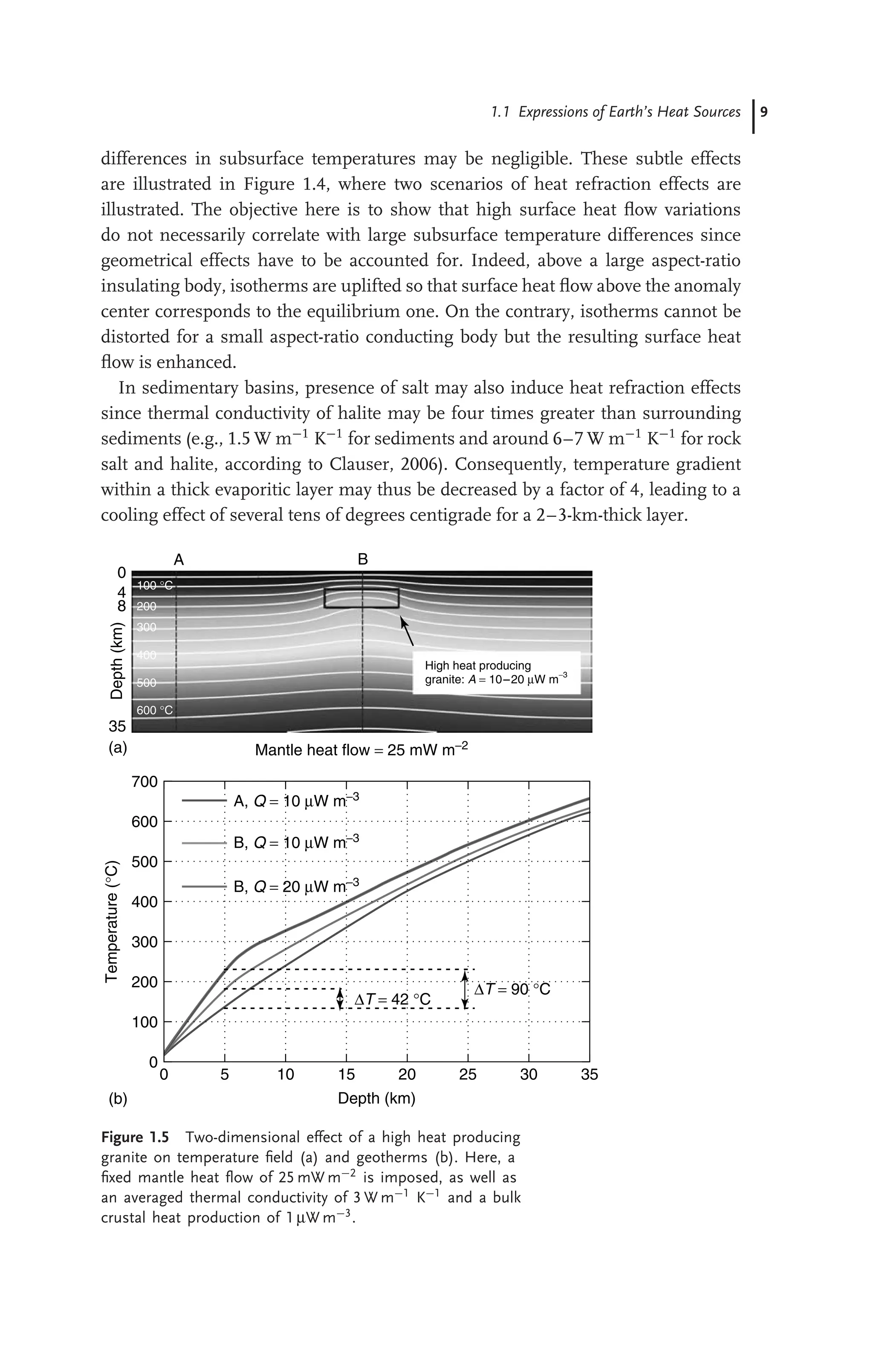
Geothermal Energy Systems Exploration Development And Utilization 1st Edition Ernst Huenges
Geothermal Energy Systems Exploration Development And Utilization 1st Edition Ernst Huenges