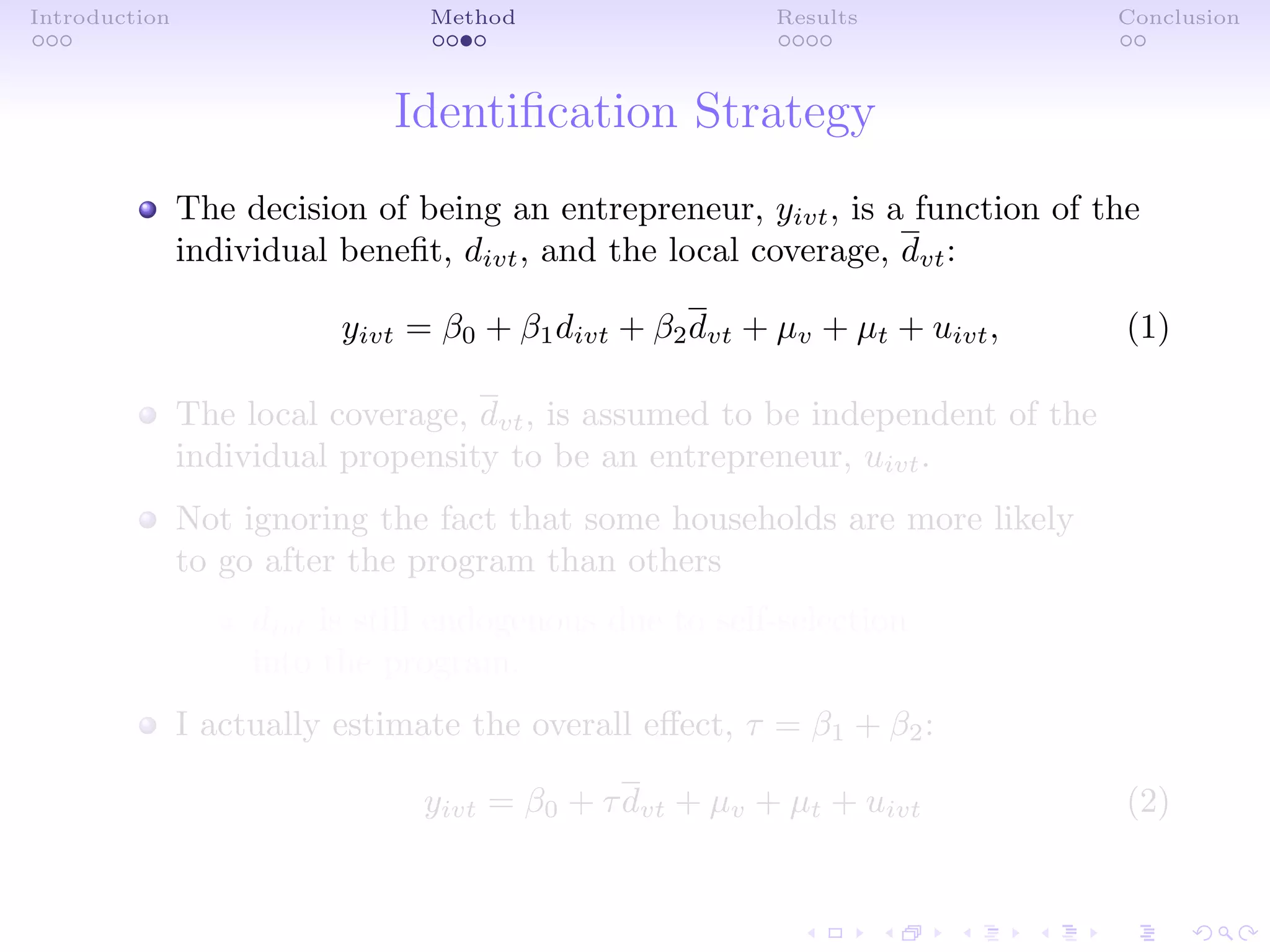
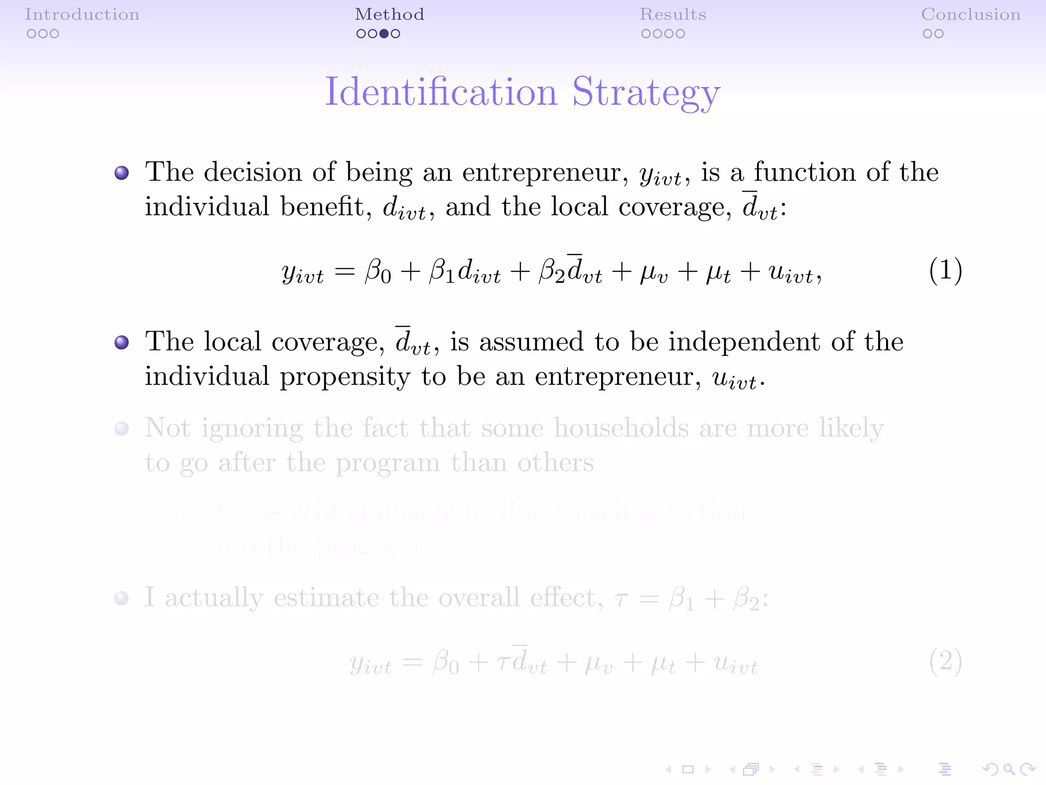
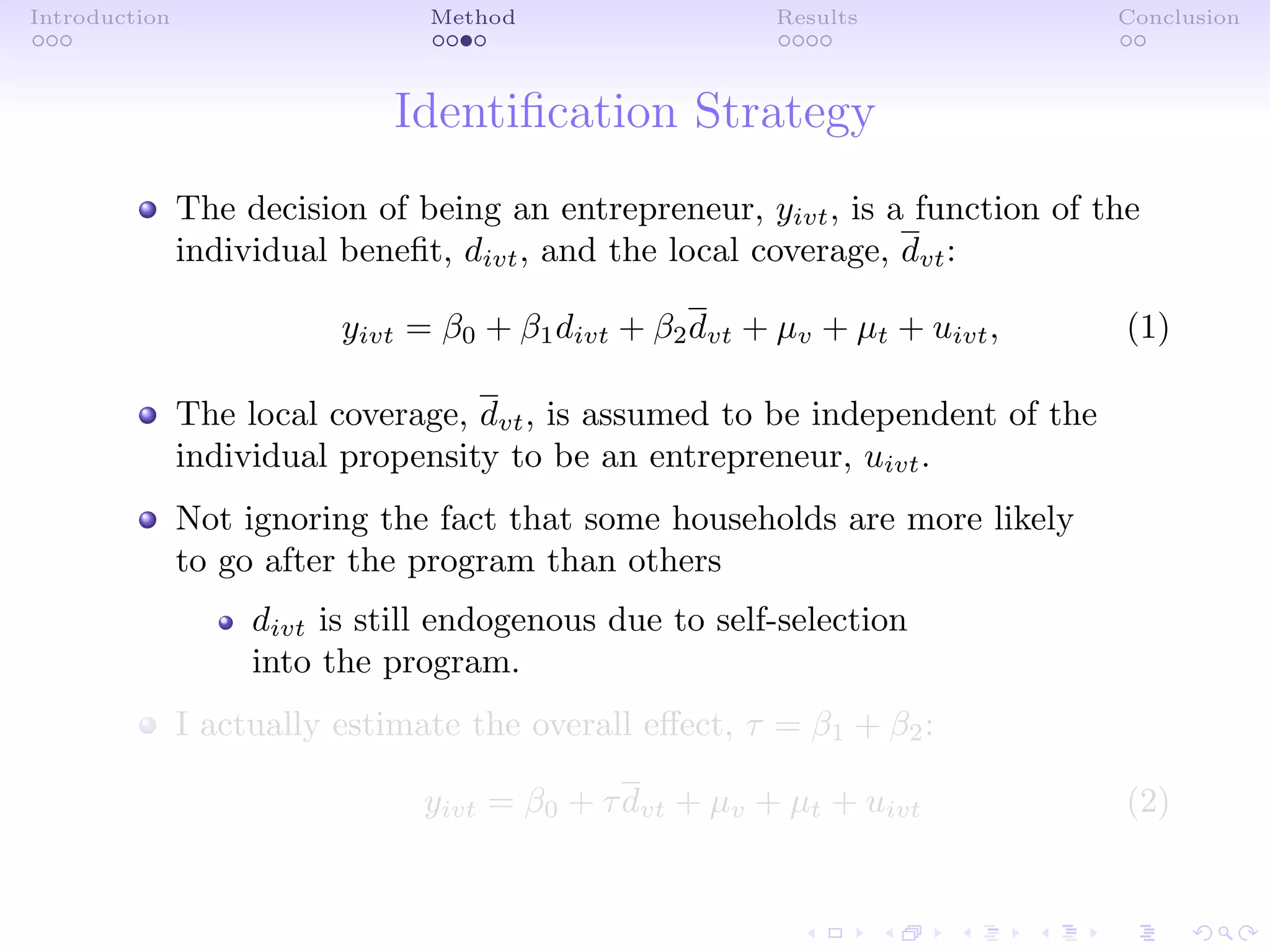
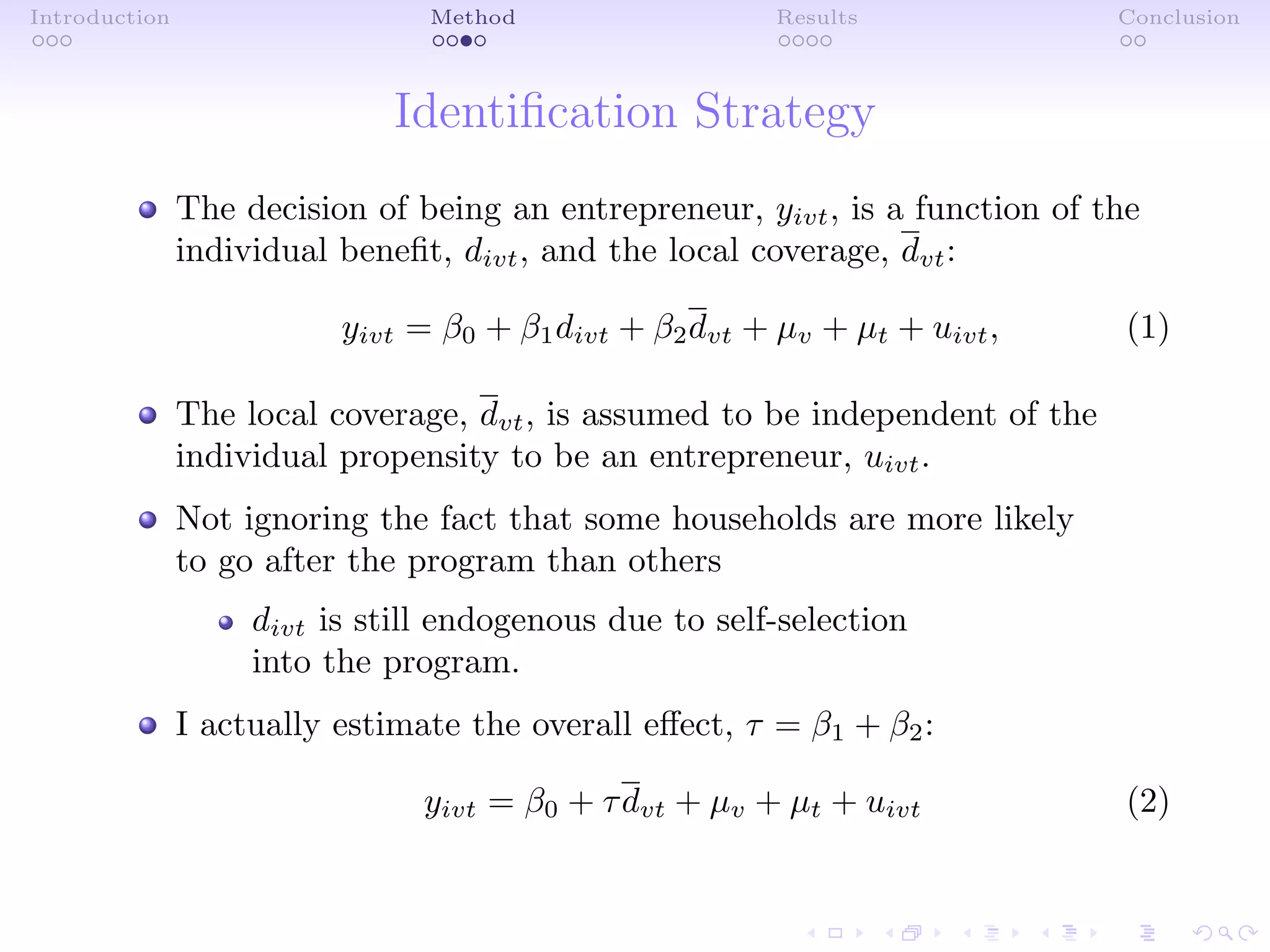
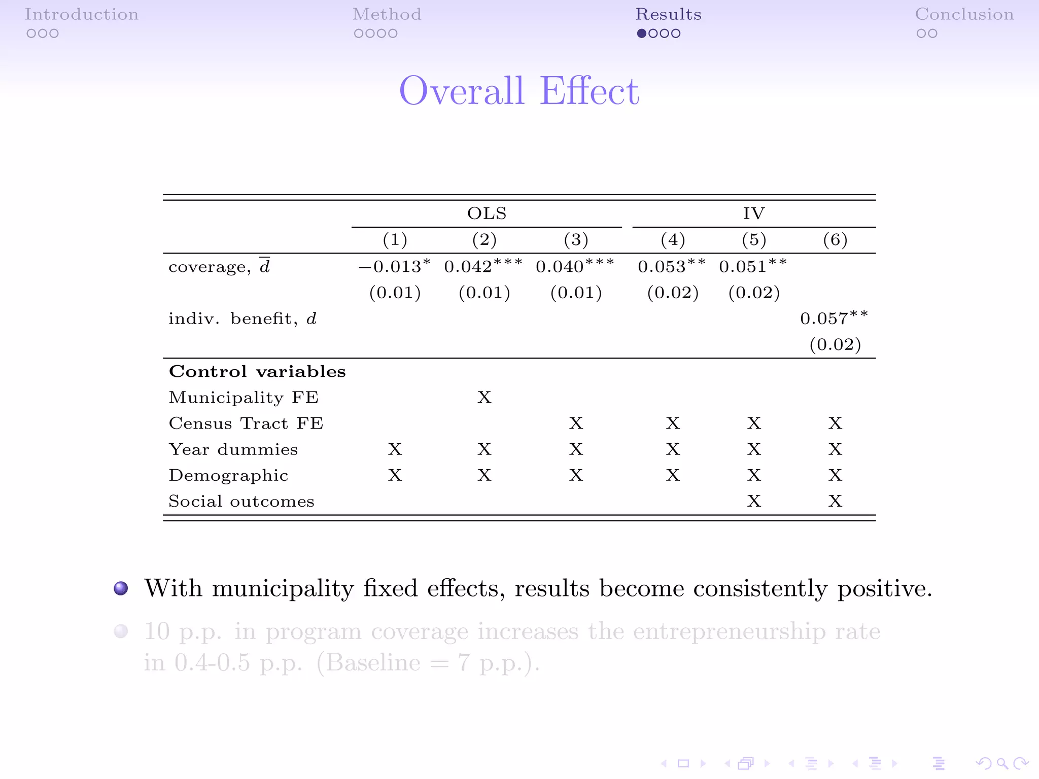
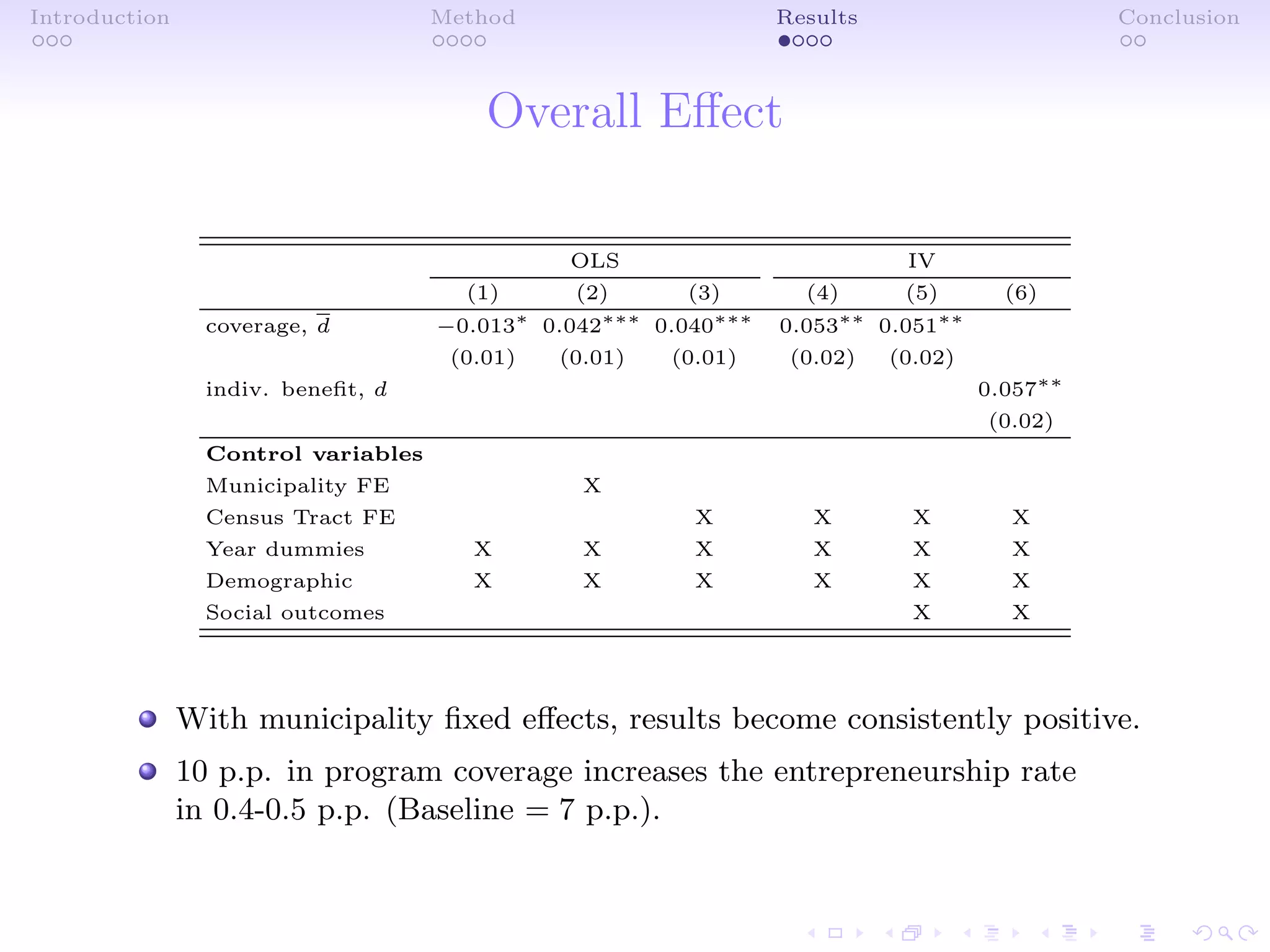
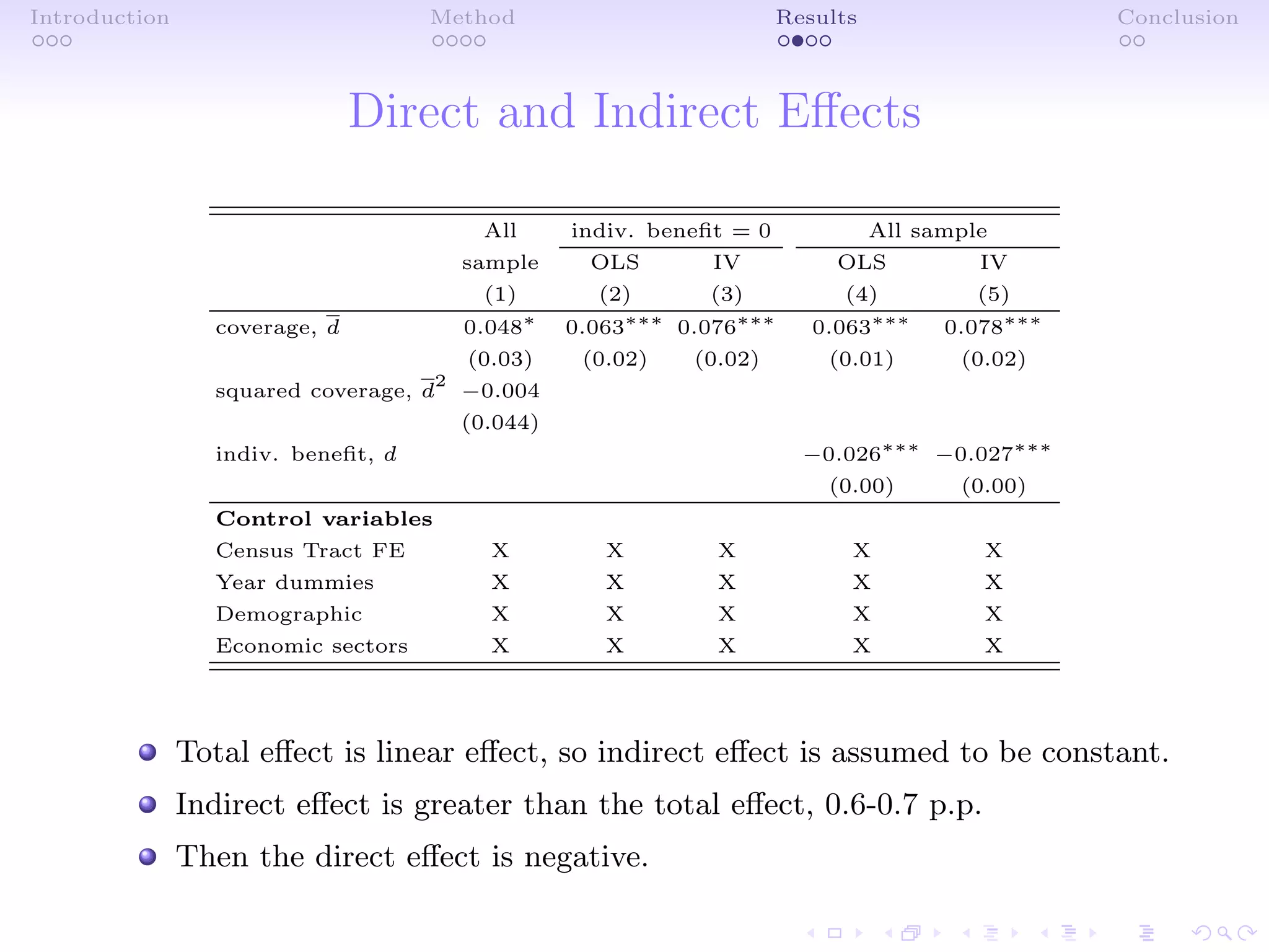
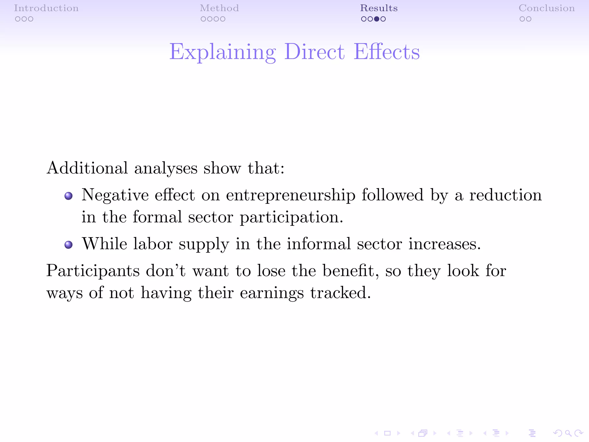
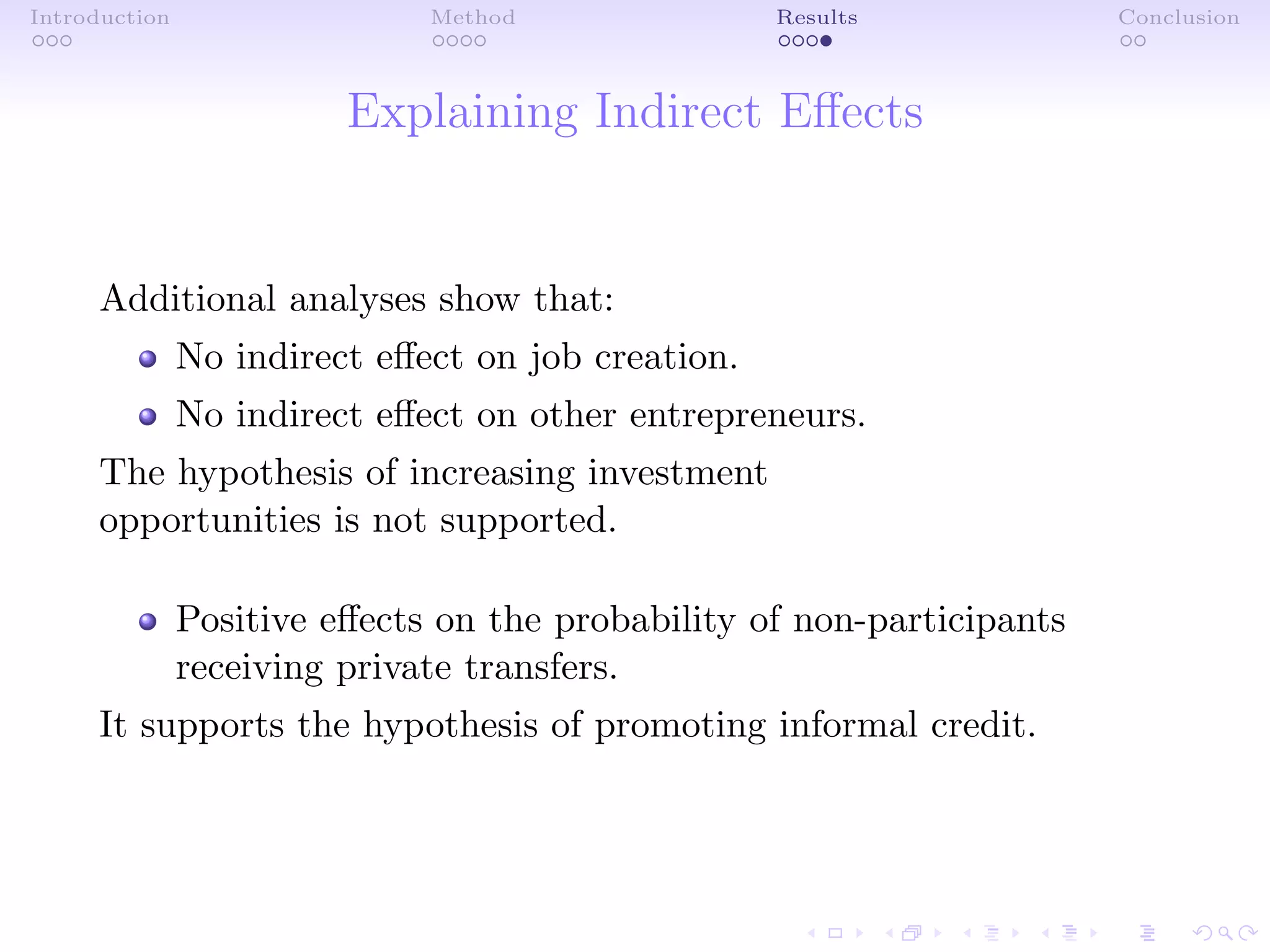
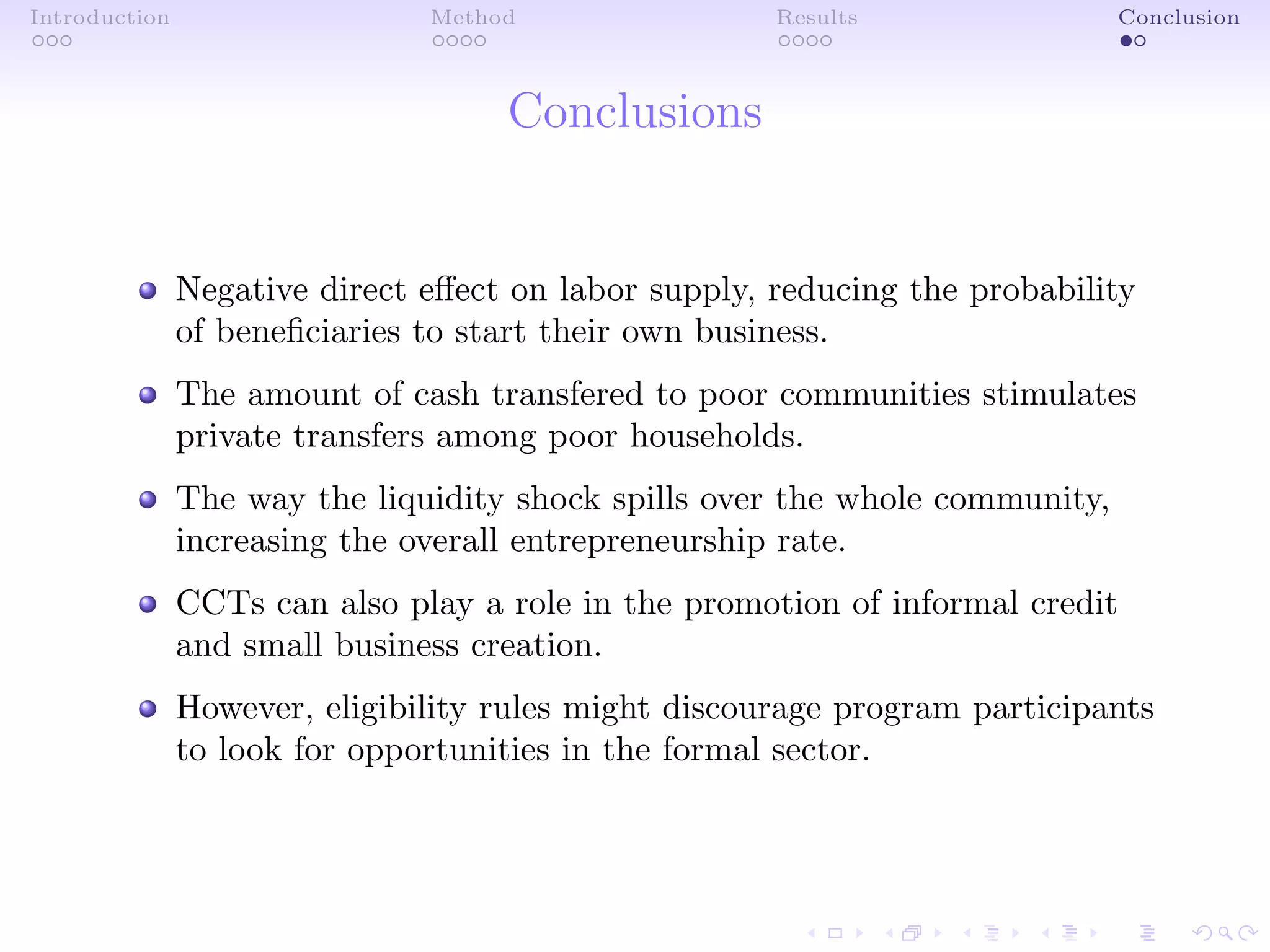
This document examines the impact of Brazil's Bolsa Família conditional cash transfer program on entrepreneurship in low-educated households. It highlights both direct effects on participants and indirect social effects, such as increased aggregate demand and informal credit availability. The findings indicate that greater program coverage correlates with increased entrepreneurship rates among participants.

1. Introduction Method Results Conclusion
Direct and Indirect Effects of
Cash Transfer on Entrepreneurship
Rafael P. Ribas
University of Illinois
GDN 14th Annual Global Development Conference,
June 20, 2013

2. Introduction Method Results Conclusion
Introduction
Capital is essential for starting a business.
Limited access to credit may lessen entrepreneurial
activity in developing countries.
The role of a liquidity shock in supporting
entrepreneurship among poor households.
Large-scale Conditional Cash Transfer (CCT) program
in Brazil, Bolsa Fam´ılia.
Conditional on school attendance and health care.
Small but steady income to poor households.
No rule over business investment or labor supply.

3. Introduction Method Results Conclusion
Introduction
Capital is essential for starting a business.
Limited access to credit may lessen entrepreneurial
activity in developing countries.
The role of a liquidity shock in supporting
entrepreneurship among poor households.
Large-scale Conditional Cash Transfer (CCT) program
in Brazil, Bolsa Fam´ılia.
Conditional on school attendance and health care.
Small but steady income to poor households.
No rule over business investment or labor supply.

4. Introduction Method Results Conclusion
Introduction
Capital is essential for starting a business.
Limited access to credit may lessen entrepreneurial
activity in developing countries.
The role of a liquidity shock in supporting
entrepreneurship among poor households.
Large-scale Conditional Cash Transfer (CCT) program
in Brazil, Bolsa Fam´ılia.
Conditional on school attendance and health care.
Small but steady income to poor households.
No rule over business investment or labor supply.

5. Introduction Method Results Conclusion
Introduction
Capital is essential for starting a business.
Limited access to credit may lessen entrepreneurial
activity in developing countries.
The role of a liquidity shock in supporting
entrepreneurship among poor households.
Large-scale Conditional Cash Transfer (CCT) program
in Brazil, Bolsa Fam´ılia.
Conditional on school attendance and health care.
Small but steady income to poor households.
No rule over business investment or labor supply.

6. Introduction Method Results Conclusion
Introduction
Capital is essential for starting a business.
Limited access to credit may lessen entrepreneurial
activity in developing countries.
The role of a liquidity shock in supporting
entrepreneurship among poor households.
Large-scale Conditional Cash Transfer (CCT) program
in Brazil, Bolsa Fam´ılia.
Conditional on school attendance and health care.
Small but steady income to poor households.
No rule over business investment or labor supply.

7. Introduction Method Results Conclusion
Introduction
Capital is essential for starting a business.
Limited access to credit may lessen entrepreneurial
activity in developing countries.
The role of a liquidity shock in supporting
entrepreneurship among poor households.
Large-scale Conditional Cash Transfer (CCT) program
in Brazil, Bolsa Fam´ılia.
Conditional on school attendance and health care.
Small but steady income to poor households.
No rule over business investment or labor supply.

8. Introduction Method Results Conclusion
Introduction
The impacts often interpreted as individual responses of
participants (direct effects),
I investigate not only the individual effect on participants,
but also the social effects.
There are two possible indirect effects:
1 Shifting the aggregate demand and
increasing investment opportunities.
2 Stimulating informal credit and private transfers.

9. Introduction Method Results Conclusion
Introduction
The impacts often interpreted as individual responses of
participants (direct effects), ignoring local spill-overs
(indirect effects).
I investigate not only the individual effect on participants,
but also the social effects.
There are two possible indirect effects:
1 Shifting the aggregate demand and
increasing investment opportunities.
2 Stimulating informal credit and private transfers.

10. Introduction Method Results Conclusion
Introduction
The impacts often interpreted as individual responses of
participants (direct effects), ignoring local spill-overs
(indirect effects).
I investigate not only the individual effect on participants,
but also the social effects.
There are two possible indirect effects:
1 Shifting the aggregate demand and
increasing investment opportunities.
2 Stimulating informal credit and private transfers.

11. Introduction Method Results Conclusion
Introduction
The impacts often interpreted as individual responses of
participants (direct effects), ignoring local spill-overs
(indirect effects).
I investigate not only the individual effect on participants,
but also the social effects.
There are two possible indirect effects:
1 Shifting the aggregate demand and
increasing investment opportunities.
2 Stimulating informal credit and private transfers.

12. Introduction Method Results Conclusion
Introduction
The impacts often interpreted as individual responses of
participants (direct effects), ignoring local spill-overs
(indirect effects).
I investigate not only the individual effect on participants,
but also the social effects.
There are two possible indirect effects:
1 Shifting the aggregate demand and
increasing investment opportunities.
2 Stimulating informal credit and private transfers.

13. Introduction Method Results Conclusion
Introduction
The impacts often interpreted as individual responses of
participants (direct effects), ignoring local spill-overs
(indirect effects).
I investigate not only the individual effect on participants,
but also the social effects.
There are two possible indirect effects:
1 Shifting the aggregate demand and
increasing investment opportunities.
2 Stimulating informal credit and private transfers.

14. Introduction Method Results Conclusion
Introduction
0
.1
.2
.3
.4
.5
.6
shareofbeneficiaries
0
.05
.1
.15
.2
.25probabilityoftransfering
1 2 3 4 5 6 7 8 9 10
Income Decile
CCT beneficiaries
non−beneficiaries
share of beneficiaries
Participants are more likely to make transfers to other households.
With more cash flowing, the individual intervention becomes social.

15. Introduction Method Results Conclusion
Introduction
0
.1
.2
.3
.4
.5
.6
shareofbeneficiaries
0
.05
.1
.15
.2
.25probabilityoftransfering
1 2 3 4 5 6 7 8 9 10
Income Decile
CCT beneficiaries
non−beneficiaries
share of beneficiaries
Participants are more likely to make transfers to other households.
With more cash flowing, the individual intervention becomes social.

16. Introduction Method Results Conclusion
Data
National Household Survey (PNAD) from 2001, 2004, 2006.
It is a cross-sectional survey, but with a
panel of neighborhoods (census tracts).
Low-educated men between 25 and 45 years,
living in urban areas.
Entrepreneurs are those either self-employed
or small business owners.
Also required that they contribute to social security.
Informal workers’ earnings cannot be tracked.

17. Introduction Method Results Conclusion
Data
National Household Survey (PNAD) from 2001, 2004, 2006.
It is a cross-sectional survey, but with a
panel of neighborhoods (census tracts).
Low-educated men between 25 and 45 years,
living in urban areas.
Entrepreneurs are those either self-employed
or small business owners.
Also required that they contribute to social security.
Informal workers’ earnings cannot be tracked.

18. Introduction Method Results Conclusion
Data
National Household Survey (PNAD) from 2001, 2004, 2006.
It is a cross-sectional survey, but with a
panel of neighborhoods (census tracts).
Low-educated men between 25 and 45 years,
living in urban areas.
Entrepreneurs are those either self-employed
or small business owners.
Also required that they contribute to social security.
Informal workers’ earnings cannot be tracked.

19. Introduction Method Results Conclusion
Data
National Household Survey (PNAD) from 2001, 2004, 2006.
It is a cross-sectional survey, but with a
panel of neighborhoods (census tracts).
Low-educated men between 25 and 45 years,
living in urban areas.
Entrepreneurs are those either self-employed
or small business owners.
Also required that they contribute to social security.
Informal workers’ earnings cannot be tracked.

20. Introduction Method Results Conclusion
Data
National Household Survey (PNAD) from 2001, 2004, 2006.
It is a cross-sectional survey, but with a
panel of neighborhoods (census tracts).
Low-educated men between 25 and 45 years,
living in urban areas.
Entrepreneurs are those either self-employed
or small business owners.
Also required that they contribute to social security.
Informal workers’ earnings cannot be tracked.

21. Introduction Method Results Conclusion
Identification Strategy
The identification assumption is inspired by the program design.
Each municipality (city or village) has a maximum number of
benefits to be offered, given by the 2000-2001 poverty rate.
R2 = 0.768
0
.2
.4
.6
.8
1
CCTcoverage
0 .2 .4 .6 .8 1
poverty headcount
2004 coverage vs. 2000 poverty
R2 = 0.916
0
.2
.4
.6
.8
1
CCTcoverage 0 .2 .4 .6 .8 1
poverty headcount
2006 coverage vs. 2000 poverty
2000 Census and Official Record
R2 = 0.742
0
.2
.4
.6
.8
1
CCTcoverage
0 .2 .4 .6 .8 1
poverty headcount
2004 coverage vs. 2001 poverty
R2 = 0.801
0
.2
.4
.6
.8
1
CCTcoverage
0 .2 .4 .6 .8 1
poverty headcount
2006 coverage vs. 2001 poverty
R2 = 0.767
0
.2
.4
.6
.8
1
CCTcoverage
0 .2 .4 .6 .8 1
poverty headcount
2006 coverage vs. 2004 poverty
National Household Survey

22. Introduction Method Results Conclusion
Identification Strategy
The identification assumption is inspired by the program design.
The growth of coverage mostly driven by the previous poverty
rate, rather than the increasing demand from poor households.
R2 = 0.768
0
.2
.4
.6
.8
1
CCTcoverage
0 .2 .4 .6 .8 1
poverty headcount
2004 coverage vs. 2000 poverty
R2 = 0.916
0
.2
.4
.6
.8
1
CCTcoverage 0 .2 .4 .6 .8 1
poverty headcount
2006 coverage vs. 2000 poverty
2000 Census and Official Record
R2 = 0.742
0
.2
.4
.6
.8
1
CCTcoverage
0 .2 .4 .6 .8 1
poverty headcount
2004 coverage vs. 2001 poverty
R2 = 0.801
0
.2
.4
.6
.8
1
CCTcoverage
0 .2 .4 .6 .8 1
poverty headcount
2006 coverage vs. 2001 poverty
R2 = 0.767
0
.2
.4
.6
.8
1
CCTcoverage
0 .2 .4 .6 .8 1
poverty headcount
2006 coverage vs. 2004 poverty
National Household Survey

23. Introduction Method Results Conclusion
Identification Strategy
The decision of being an entrepreneur, yivt, is a function of the
individual benefit, divt, and the local coverage, dvt:
yivt = β0 + β1divt + β2dvt + µv + µt + uivt, (1)
The local coverage, dvt, is assumed to be independent of the
individual propensity to be an entrepreneur, uivt.
Not ignoring the fact that some households are more likely
to go after the program than others
divt is still endogenous due to self-selection
into the program.
I actually estimate the overall effect, τ = β1 + β2:
yivt = β0 + τdvt + µv + µt + uivt (2)

24. Introduction Method Results Conclusion
Identification Strategy
The decision of being an entrepreneur, yivt, is a function of the
individual benefit, divt, and the local coverage, dvt:
yivt = β0 + β1divt + β2dvt + µv + µt + uivt, (1)
The local coverage, dvt, is assumed to be independent of the
individual propensity to be an entrepreneur, uivt.
Not ignoring the fact that some households are more likely
to go after the program than others
divt is still endogenous due to self-selection
into the program.
I actually estimate the overall effect, τ = β1 + β2:
yivt = β0 + τdvt + µv + µt + uivt (2)

25. Introduction Method Results Conclusion
Identification Strategy
The decision of being an entrepreneur, yivt, is a function of the
individual benefit, divt, and the local coverage, dvt:
yivt = β0 + β1divt + β2dvt + µv + µt + uivt, (1)
The local coverage, dvt, is assumed to be independent of the
individual propensity to be an entrepreneur, uivt.
Not ignoring the fact that some households are more likely
to go after the program than others
divt is still endogenous due to self-selection
into the program.
I actually estimate the overall effect, τ = β1 + β2:
yivt = β0 + τdvt + µv + µt + uivt (2)

26. Introduction Method Results Conclusion
Identification Strategy
The decision of being an entrepreneur, yivt, is a function of the
individual benefit, divt, and the local coverage, dvt:
yivt = β0 + β1divt + β2dvt + µv + µt + uivt, (1)
The local coverage, dvt, is assumed to be independent of the
individual propensity to be an entrepreneur, uivt.
Not ignoring the fact that some households are more likely
to go after the program than others
divt is still endogenous due to self-selection
into the program.
I actually estimate the overall effect, τ = β1 + β2:
yivt = β0 + τdvt + µv + µt + uivt (2)

27. Introduction Method Results Conclusion
Separating Direct and Indirect Effects
If the indirect effect, β2, is different for participants
and non-participants, then the overall effect, τ, must be
nonlinear.
Then the sample of non-participants is used
to estimate the indirect effect.
The direct effect is the biased estimate minus expected bias:
˜β1 = ˆβ1 − ˆτ(d=0) − ˆβ2 .
All coefficients are estimated using seemingly unrelated
regressions (SUR).

28. Introduction Method Results Conclusion
Separating Direct and Indirect Effects
If the indirect effect, β2, is different for participants
and non-participants, then the overall effect, τ, must be
nonlinear.
Then the sample of non-participants is used
to estimate the indirect effect.
The direct effect is the biased estimate minus expected bias:
˜β1 = ˆβ1 − ˆτ(d=0) − ˆβ2 .
All coefficients are estimated using seemingly unrelated
regressions (SUR).

29. Introduction Method Results Conclusion
Separating Direct and Indirect Effects
If the indirect effect, β2, is different for participants
and non-participants, then the overall effect, τ, must be
nonlinear.
Then the sample of non-participants is used
to estimate the indirect effect.
The direct effect is the biased estimate minus expected bias:
˜β1 = ˆβ1 − ˆτ(d=0) − ˆβ2 .
All coefficients are estimated using seemingly unrelated
regressions (SUR).

30. Introduction Method Results Conclusion
Separating Direct and Indirect Effects
If the indirect effect, β2, is different for participants
and non-participants, then the overall effect, τ, must be
nonlinear.
Then the sample of non-participants is used
to estimate the indirect effect.
The direct effect is the biased estimate minus expected bias:
˜β1 = ˆβ1 − ˆτ(d=0) − ˆβ2 .
All coefficients are estimated using seemingly unrelated
regressions (SUR).

31. Introduction Method Results Conclusion
Overall Effect
OLS IV
(1) (2) (3) (4) (5) (6)
coverage, d −0.013∗
0.042∗∗∗
0.040∗∗∗
0.053∗∗
0.051∗∗
(0.01) (0.01) (0.01) (0.02) (0.02)
indiv. benefit, d 0.057∗∗
(0.02)
Control variables
Municipality FE X
Census Tract FE X X X X
Year dummies X X X X X X
Demographic X X X X X X
Social outcomes X X
With municipality fixed effects, results become consistently positive.
10 p.p. in program coverage increases the entrepreneurship rate
in 0.4-0.5 p.p. (Baseline = 7 p.p.).

32. Introduction Method Results Conclusion
Overall Effect
OLS IV
(1) (2) (3) (4) (5) (6)
coverage, d −0.013∗
0.042∗∗∗
0.040∗∗∗
0.053∗∗
0.051∗∗
(0.01) (0.01) (0.01) (0.02) (0.02)
indiv. benefit, d 0.057∗∗
(0.02)
Control variables
Municipality FE X
Census Tract FE X X X X
Year dummies X X X X X X
Demographic X X X X X X
Social outcomes X X
With municipality fixed effects, results become consistently positive.
10 p.p. in program coverage increases the entrepreneurship rate
in 0.4-0.5 p.p. (Baseline = 7 p.p.).

33. Introduction Method Results Conclusion
Direct and Indirect Effects
All indiv. benefit = 0 All sample
sample OLS IV OLS IV
(1) (2) (3) (4) (5)
coverage, d 0.048∗
0.063∗∗∗
0.076∗∗∗
0.063∗∗∗
0.078∗∗∗
(0.03) (0.02) (0.02) (0.01) (0.02)
squared coverage, d
2
−0.004
(0.044)
indiv. benefit, d −0.026∗∗∗
−0.027∗∗∗
(0.00) (0.00)
Control variables
Census Tract FE X X X X X
Year dummies X X X X X
Demographic X X X X X
Economic sectors X X X X X
Total effect is linear effect, so indirect effect is assumed to be constant.
Indirect effect is greater than the total effect, 0.6-0.7 p.p.
Then the direct effect is negative.

34. Introduction Method Results Conclusion
Direct and Indirect Effects
All indiv. benefit = 0 All sample
sample OLS IV OLS IV
(1) (2) (3) (4) (5)
coverage, d 0.048∗
0.063∗∗∗
0.076∗∗∗
0.063∗∗∗
0.078∗∗∗
(0.03) (0.02) (0.02) (0.01) (0.02)
squared coverage, d
2
−0.004
(0.044)
indiv. benefit, d −0.026∗∗∗
−0.027∗∗∗
(0.00) (0.00)
Control variables
Census Tract FE X X X X X
Year dummies X X X X X
Demographic X X X X X
Economic sectors X X X X X
Total effect is linear effect, so indirect effect is assumed to be constant.
Indirect effect is greater than the total effect, 0.6-0.7 p.p.
Then the direct effect is negative.

35. Introduction Method Results Conclusion
Explaining Direct Effects
Additional analyses show that:
Negative effect on entrepreneurship followed by a reduction
in the formal sector participation.
While labor supply in the informal sector increases.

36. Introduction Method Results Conclusion
Explaining Direct Effects
Additional analyses show that:
Negative effect on entrepreneurship followed by a reduction
in the formal sector participation.
While labor supply in the informal sector increases.

37. Introduction Method Results Conclusion
Explaining Direct Effects
Additional analyses show that:
Negative effect on entrepreneurship followed by a reduction
in the formal sector participation.
While labor supply in the informal sector increases.

38. Introduction Method Results Conclusion
Explaining Direct Effects
Additional analyses show that:
Negative effect on entrepreneurship followed by a reduction
in the formal sector participation.
While labor supply in the informal sector increases.
Participants don’t want to lose the benefit, so they look for
ways of not having their earnings tracked.

39. Introduction Method Results Conclusion
Explaining Indirect Effects
Additional analyses show that:
No indirect effect on job creation.
No indirect effect on other entrepreneurs.
Positive effects on the probability of non-participants
receiving private transfers.

40. Introduction Method Results Conclusion
Explaining Indirect Effects
Additional analyses show that:
No indirect effect on job creation.
No indirect effect on other entrepreneurs.
Positive effects on the probability of non-participants
receiving private transfers.

41. Introduction Method Results Conclusion
Explaining Indirect Effects
Additional analyses show that:
No indirect effect on job creation.
No indirect effect on other entrepreneurs.
The hypothesis of increasing investment
opportunities is not supported.
Positive effects on the probability of non-participants
receiving private transfers.

42. Introduction Method Results Conclusion
Explaining Indirect Effects
Additional analyses show that:
No indirect effect on job creation.
No indirect effect on other entrepreneurs.
The hypothesis of increasing investment
opportunities is not supported.
Positive effects on the probability of non-participants
receiving private transfers.
It supports the hypothesis of promoting informal credit.

43. Introduction Method Results Conclusion
Conclusions
Negative direct effect on labor supply, reducing the probability
of beneficiaries to start their own business.
The amount of cash transfered to poor communities stimulates
private transfers among poor households.
The way the liquidity shock spills over the whole community,
increasing the overall entrepreneurship rate.
CCTs can also play a role in the promotion of informal credit
and small business creation.
However, eligibility rules might discourage program participants
to look for opportunities in the formal sector.

44. Introduction Method Results Conclusion
Conclusions
Negative direct effect on labor supply, reducing the probability
of beneficiaries to start their own business.
The amount of cash transfered to poor communities stimulates
private transfers among poor households.
The way the liquidity shock spills over the whole community,
increasing the overall entrepreneurship rate.
CCTs can also play a role in the promotion of informal credit
and small business creation.
However, eligibility rules might discourage program participants
to look for opportunities in the formal sector.

45. Introduction Method Results Conclusion
Conclusions
Negative direct effect on labor supply, reducing the probability
of beneficiaries to start their own business.
The amount of cash transfered to poor communities stimulates
private transfers among poor households.
The way the liquidity shock spills over the whole community,
increasing the overall entrepreneurship rate.
CCTs can also play a role in the promotion of informal credit
and small business creation.
However, eligibility rules might discourage program participants
to look for opportunities in the formal sector.

46. Introduction Method Results Conclusion
Conclusions
Negative direct effect on labor supply, reducing the probability
of beneficiaries to start their own business.
The amount of cash transfered to poor communities stimulates
private transfers among poor households.
The way the liquidity shock spills over the whole community,
increasing the overall entrepreneurship rate.
CCTs can also play a role in the promotion of informal credit
and small business creation.
However, eligibility rules might discourage program participants
to look for opportunities in the formal sector.

47. Introduction Method Results Conclusion
Thank you for your attention
Rafael P. Ribas
rpribas.rs@gmail.com
http://publish.illinois.edu/ribas1