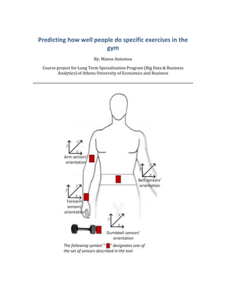
The document summarizes research on using predictive modeling to predict how well people perform specific exercises at the gym based on data from wearable sensors. It describes applying classification tree and random forest models to a dataset containing sensor data from participants performing bicep curls. Classification trees work by recursively splitting the data into partitions to predict the exercise class, while random forests create many classification trees and have the trees vote to make predictions. The models were able to accurately predict the exercise class based on the sensor data.
Deep Learning - Hype, Reality and Applications in ManufacturingAdam Cook
This is the slide deck for the introductory webinar for our "Artificial Intelligence in Manufacturing" webinar and workshop series within the SME Virtual Network.
The video for this slide deck is located here: https://www.youtube.com/watch?v=orrVqOnFqds
To learn more about the SME Virtual Network and our events, please visit the following links:
https://www.facebook.com/smevirtual/
https://www.linkedin.com/company/smevirtual/
How to implement artificial intelligence solutionsCarlos Toxtli
In this presentation, we show how a novice can learn artificial intelligence and implement the basic principles in real-world solutions. There is an easy quick start guide.
Artificial intelligence in practice- part-1GMR Group
Summary is made in 5 parts-
This is Part -1
Cyber-solutions to real-world business problems Artificial Intelligence in Practice is a fascinating look into how companies use AI and machine learning to solve problems. Presenting 50 case studies of actual situations, this book demonstrates practical applications to issues faced by businesses around the globe.
• The rapidly evolving field of artificial intelligence has expanded beyond research labs and computer science departments and made its way into the mainstream business environment.
• Artificial intelligence and machine learning are cited as the most important modern business trends to drive success.
• It is used in areas ranging from banking and finance to social media and marketing.
• This technology continues to provide innovative solutions to businesses of all sizes, sectors and industries.
• This engaging and topical book explores a wide range of cases illustrating how businesses use AI to boost performance, drive efficiency, analyse market preferences and many others.
• This detailed examination provides an overview of each company, describes the specific problem and explains how AI facilitates resolution.
• Each case study provides a comprehensive overview, including some technical details as well as key learning summaries:
o Understand how specific business problems are addressed by innovative machine learning methods Explore how current artificial intelligence applications improve performance and increase efficiency in various situations
o Expand your knowledge of recent AI advancements in technology
o Gain insight on the future of AI and its increasing role in business and industry
o Artificial Intelligence in Practice: How 50 Successful Companies Used Artificial Intelligence to Solve Problems is an insightful and informative exploration of the trans-formative power of technology in 21st century commerce
I made this presentation in my 7th semester of B.Tech as per academic curriculum.
Took help from several videos from youtube and studied some IBM publications.
Cognitive Era is at the dawn. It does not make machines intelligent but instead it allows them to develop cognisance and learn by themselves as we humans do.
I am fascinated and looking forward to contribute my existence in this great thought of almighty came into human mind.
Guys! You could get a nice introduction from this presentation and explain it to others and even it could be used for your academic homework.
Goodluck! GODSPEED!
As we move forward into the digital age, One of the modern innovations we’ve seen is the creation of Machine Learning. This incredible form of artificial intelligence is already being used in various industries and professions. For Example, Image and Speech Recognition, Medical Diagnosis, Prediction, Classification, Learning Associations, Statistical Arbitrage, Extraction, Regression. Today we’re looking at all these Machine Learning Applications in today’s modern world.
AI in Healthcare: How to Implement Medical Imaging Using Machine Learning?Skyl.ai
About the webinar
According to a report “The Digital Universe Driving Data Growth in Healthcare,” published by EMC with research and analysis from IDC, Hospitals are producing 50 petabytes of data per year. Almost 90% of this data is comprised of medical imaging i.e. digital images from scans like MRIs or CTs. More than 97% of this data goes unanalyzed or unused.
The top healthcare institutions across the globe are adopting AI in medical imaging to increase speed and imaging accuracy, monitor data in real-time, and eliminate the need for humans to do time-consuming and complex tasks. This has been enabling doctors to optimize treatment approaches, speed of care, and interconnected health conditions.
Through this webinar, you will understand how AI can be used to automate routine processes and procedures and help radiologists to identify patterns, and help in treating patients with critical conditions quickly.
What you will learn:
- How healthcare institutions are leveraging AI to augment decision making, prevent medical errors, and reduce costs in medical imaging
- Discuss the approach to automate machine learning workflow, creating and deploying models in hours, not weeks or months
- Demo: How to detect pneumonia from chest x-rays using AI within a few minutes using skyl.ai
For many, it's a nebulous term that invokes images of huge server farms humming away. Or perhaps you think of receiving some kind of personalized advertisement from a retailer. But big data is so much deeper and broader than that. Read this post to know more http://www.lanterninstitute.ca
AI & Cognitive Computing are some of the most popular business an technical words out there. It is critical to get the basic understanding of Cognitive Computing, which helps us appreciate the technical possibilities and business benefits of the technology.
Data Science has become one of the most demanded jobs of the 21st century. It has become a buzzword that almost everyone talks about these days. But what is Data Science? In this article, we will demystify Data Science, the role of a Data Scientist and have a look at the tools required to master Data Science.
1. Predicting how well people do specific exercises in the
gym
By: Manos Antoniou
Course project for Long Term Specialization Program (Big Data & Business
Analytics) of Athens University of Economics and Business
2. 1
TABLE OF CONTENTS
Introduction………………………………………………..Page 01
Human Activity Recognition…………………………Page 01
Predictive modeling…………………………………….Page 02
Data Analysis Environment…………………………..Page 03
Dataset Description……………………………………..Page 04
Data Cleaning/Exploratory Analysis……………..Page 04
Predictive Modelling (Classification Trees)……Page 06
Predictive Modelling (Random Forest)………….Page 08
Modelling in R……………………………………………..Page 11
R Code & Output………………………………………….Page 12
Results & Conclusions…………………………………..Page 17
Bibliography………………………………………………..Page 18
Introduction
The main scope of this course project is to investigate if & how we can predict the
manner in which people did some specific exercise in the gym, by using
wearable device (with sensors). In order to investigate this, predictive modelling
methods have been applied. A successful prediction will help people have less
injuries and better work-out routines, without the need of constant presence of a
fitness instructor.
HAR(Human Activity Recognition)
Human Activity Recognition (HAR) has emerged as a key research area in the last
years and is gaining increasing attention by the pervasive computing research,
especially for the development of context-aware systems.
New era of computing
Computers are becoming more pervasive, as they are embedded in our phones,
music players, cameras, in clothing, in buildings, cars, and in all kinds of everyday
objects which do not resemble our long-established image of a desktop PC with a
screen, keyboard and mouse. How should we interact and live with many computers
that are small, and sometimes hidden so that we cannot even see them? In which
ways can they make our lives better? The vision of ubiquitous computing is that,
eventually, computers will disappear and become part of our environment, fading
into the background of our everyday lives. Ideally, there will be more computers,
invisibly enhancing our surroundings, but we will be less aware of them,
concentrating on our tasks instead of the technology. As designers of ubiquitous
computing technologies, we are challenged to find new ways to interact with this
new generation of computers, and new uses for them. One way of making computers
3. 2
disappear is to reduce the amount of explicit interaction that is needed to
communicate with them, and instead increase the amount of implicit interaction.
Sensors
Human activities are so diverse that there does not exist one single type of sensor
that could recognize all of them. For example, while physical motion can be well-
recognized by inertial sensors, other activities, such as talking, reading, chewing, or
physiological states of the user, can be better recognized with other, sometimes
dedicated sensors. Making sensors less obtrusive, more robust, easier to use,
washable, even attractive, are other challenges which are addressed.
Wearable devices
Using devices such as Jawbone Up, Nike Fuel Band, and Fitbit it is now possible to
collect a large amount of data about human activity relatively inexpensively. These
type of devices are part of the quantified self movement – a group of enthusiasts
who take measurements about themselves regularly to improve their health, to find
patterns in their behavior, or because they are tech geeks. One thing that people
regularly do is quantify how much of a particular activity they do, but they rarely
quantify how well they do it.
Predictive modeling
From telecoms to finance, e-commerce to government, predictive models are being
utilized across various sectors to tackle all kinds of business problems. For
thousands of years, people have had the desire to (or claimed they could) predict
the future. This desire to foresee what lies down the road is a common one among
individuals, each of us wanting to know what our lives will be like one day.
Naturally, companies also possess this desire, wanting to know whether certain
products or services they plan on releasing will be successful, whether their
customer base will expand or shrink based on a strategic decision, or whether their
investments will pan out as desired. Thankfully, the rise of the digital era has
partially enabled this, (with the help of databases and the power of analytics), taking
shape in the form of predictive modeling.
Predictive modeling, by definition, is the analysis of current and historical facts to
make predictions about future events. Several techniques – according to the nature
of the business problem and current conditions – can be used when conducting
predictive modeling. These include regression techniques, time series models,
decision trees, and machine learning methods, among others.
The phases of predictive modeling are rather straightforward, and involve activities
aimed at ensuring a look into the past through the analysis of various data points
will in fact help predict the future:
4. 3
Telecom companies, use predictive modeling to predict customer demand for
voice or data services by predicting churn.
Financial Institutions & Banks use predictive modeling techniques to estimate the
potential value of a given customer over their entire lifetime or estimate the
likelihood of a loan being defaulted on by looking at several variables.
Marketeers and Advertisers, use predictive modeling to identify the most
appropriate individuals to target for each specific campaign that will be launched.
E-commerce sites such as Amazon or Netflix, use “recommendations” systems to
determine the next best offer to their customers. Netflix declared that from 1999 to
2006, revenues generated directly from the practice of analyzing customer behavior
and creating customized offerings increased from $5 million to $1 billion dollars.
Almost all of us use spam e-mail filtering. Predictive modeling techniques are used
extensively in helping to determine which e-mails are more likely to be junk. We
may not be aware, but Google, Microsoft, Apple e.t.c are using spam filters on their
products.
Health Care Institutes improving care services. New York City Health and Hospital
Corporation uses predictive modeling to predict disease related risks for each of its
members.
Government is predicting equipment failure. The US Army has created several
predictive models for the purpose of estimating how and when the various
equipment it has on hand will fail.
Data Analysis Enviroment
All data analysis was conducted with R. It is a programming language and software
environment for statistical computing and graphics. The R language is widely used
among statisticians and data miners for developing statistical software and data
analysis. R is a GNU project. The source code for the R software environment is
written primarily in C, Fortran, and R.It is freely available under the GNU General
Public License, and pre-compiled binary versions are provided for various operating
systems.
5. 4
Dataset Description
The dataset was collected from accelerometers on the belt, forearm, arm, and
dumbbell of six young health participants. They were asked to perform one set of 10
repetitions of the Unilateral Dumbbell Biceps Curl in five different fashions:
• Exactly according to the specification (Class A)
• Throwing the elbows to the front (Class B)
• Lifting the dumbbell only halfway (Class C)
• Lowering the dumbbell only halfway (Class D)
• Throwing the hips to the front (Class E)
Class A corresponds to the specified execution of the exercise, while the other 4
classes correspond to common mistakes. Participants were supervised by an
experienced weight lifter to make sure the execution complied to the manner they
were supposed to simulate. The exercises were performed by six male participants
aged between 20-28 years, with little weight lifting experience. All participants
could easily simulate the mistakes in a safe and controlled manner by using a
relatively light dumbbell (1.25kg).
The challenge is to predict the manner in which they did the exercise. We want to
investigate "how well" an activity was performed by the wearer. It potentially
provides useful information for a large variety of applications, such as sports
training.
This dataset is licensed under the Creative Commons license (CC BY-SA). Read more:
http://groupware.les.inf.puc-rio.br/har#ixzz3dWHkhIUo
Data Cleaning/Exploratory Analysis
The following script is used to import the dataset.
# Load all R Libraries that will be required for all the analysis
library(ggplot2)
library(ElemStatLearn)
library(caret)
library(randomForest)
library(rattle)
library(rpart.plot)
# Check if file exists on working directory and if not, it downloads it
and
# saves it as data.csv
if (!file.exists("data.csv")) {
6. 5
fileUrl <- "http://groupware.les.inf.puc-rio.br/static/WLE/Wear
ableComputing_weight_lifting_exercises_biceps_curl_variations.csv"
download.file(fileUrl, destfile="./data.csv")
}
# Insert the dataset in R enviroment by converting all null values
# to missing values (NA's)
data <- read.csv("data.csv", header = TRUE, sep = ",", quote = """, na
.strings=c("NA",""))
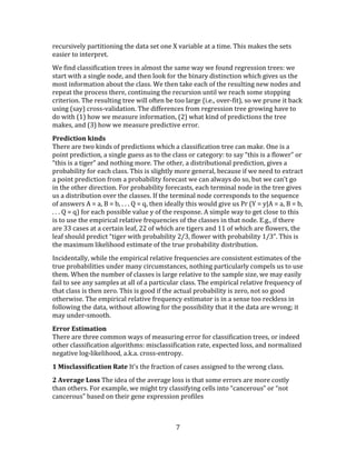
There are 39242 observations and 159 variables in the dataset. It is important to
check if all variables are useful or if we can ignore some, in order to produce a more
accurate prediction model.
Firstly, we can ignore the first 6 variables as they don't include any actual measure
data. Then it's very important to have a look on how many missing values each
column has. It appears that 100 variables consist of more than 98%
missing values. On the other hand, the remaining 59 have almost none. It is clear
that we have to ignore all 100 variables with the missing values and the first 6
variables. So the final "processed" dataset will consist of 53 variables. The
following script includes the appropriate R code
# Create a dataframe with the sum of missing values per column
data.na <- as.data.frame(apply(X=data,2,FUN=function(x) length(which(is
.na(x)))))
names(data.na) <- "Missing Values"
# Keep the columns that contain Non-missing values (NA's)
data1 <- data[,colSums(is.na(data)) < 2]
# Delete the first 7 columns, because they are not important for the pr
edictive
# modelling
data1 <- data1[,7:59]
# Exclude remaining rows that contains missing data
data1 <- na.omit(data1)
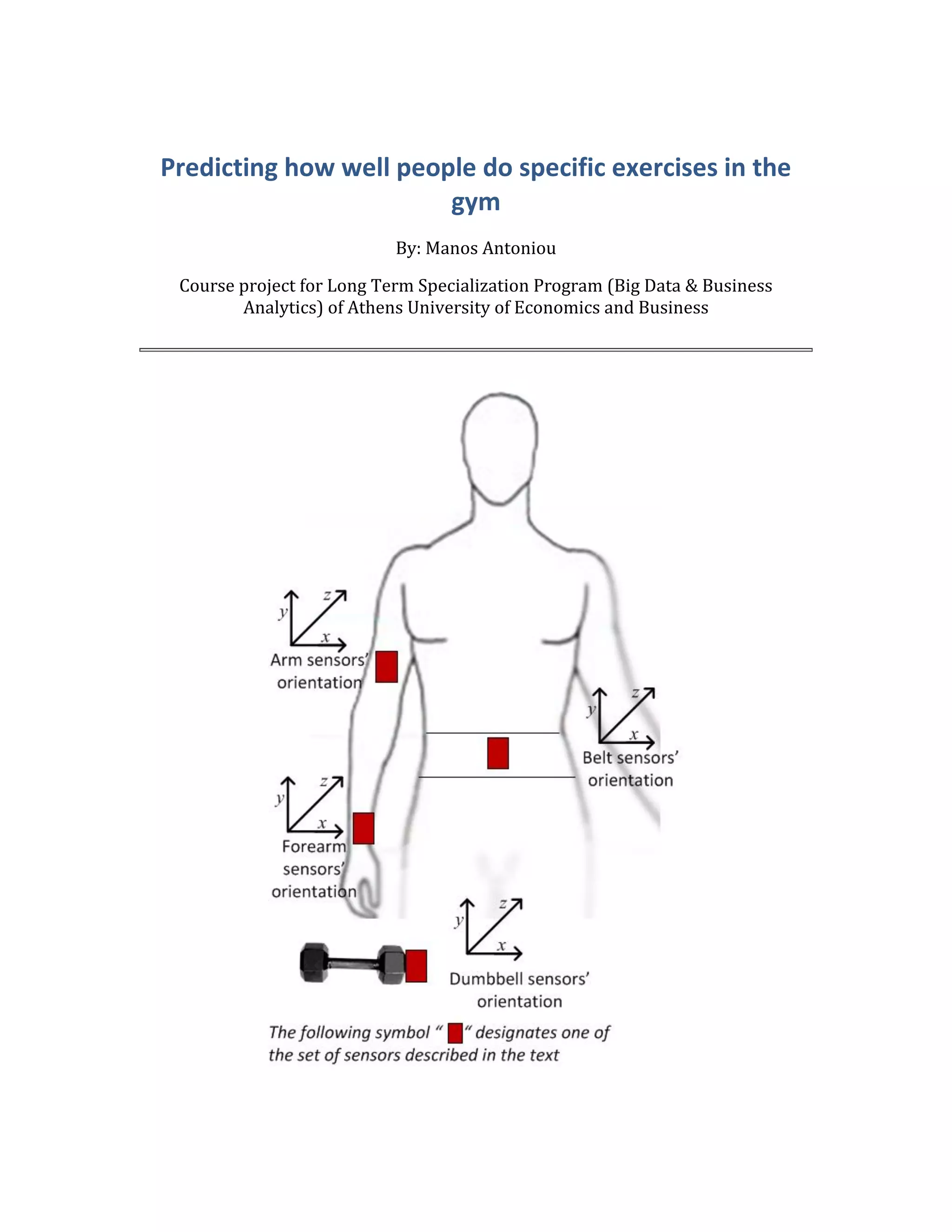
So the final dataset consists of 39241 observations and 53 variables. It is also
important to check how many observations of each class outcome exist. There are
more than 11000 observations with class "A" as outcome and around 6500-7500
observations for each of the rest classes (B,C,D,E) which is not bad (enough cases
from each class).
7. 6
Predictive Modelling
Two different approaches were used for developing the prediction algorithm. The
first one is classification trees and the second is random forest.
Classification Trees
Classification trees are machine-learning methods for constructing prediction
models from data. The models are obtained by recursively partitioning the data
space and fitting a simple prediction model within each partition. As a result, the
partitioning can be represented graphically as a decision tree. Classification trees
are designed for dependent variables that take a finite number of un-ordered values,
with prediction error measured in terms of misclassification cost.
How it works
In a classification problem, we have a training sample of n observations on a class
variable Y that takes values 1, 2, ... , k, and p predictor variables, X1,..., Xp. Our goal is
to find a model for predicting the values of Y from new X values. In theory, the
solution is simply a partition of the X space into k disjoint sets, A1, A2,..., Ak, such
that the predicted value of Y is j if X belongs to Aj , for j = 1, 2,..., k.
If the X variables take ordered values, two classical solutions are linear discriminant
analysis and nearest neighbor classification. These methods yield sets Aj with
piecewise linear and nonlinear, respectively, boundaries that are not easy to
interpret if p is large. Classification tree methods yield rectangular sets Aj by
8. 7
recursively partitioning the data set one X variable at a time. This makes the sets
easier to interpret.
We find classification trees in almost the same way we found regression trees: we
start with a single node, and then look for the binary distinction which gives us the
most information about the class. We then take each of the resulting new nodes and
repeat the process there, continuing the recursion until we reach some stopping
criterion. The resulting tree will often be too large (i.e., over-fit), so we prune it back
using (say) cross-validation. The differences from regression tree growing have to
do with (1) how we measure information, (2) what kind of predictions the tree
makes, and (3) how we measure predictive error.
Prediction kinds
There are two kinds of predictions which a classification tree can make. One is a
point prediction, a single guess as to the class or category: to say “this is a flower” or
“this is a tiger” and nothing more. The other, a distributional prediction, gives a
probability for each class. This is slightly more general, because if we need to extract
a point prediction from a probability forecast we can always do so, but we can’t go
in the other direction. For probability forecasts, each terminal node in the tree gives
us a distribution over the classes. If the terminal node corresponds to the sequence
of answers A = a, B = b, . . . Q = q, then ideally this would give us Pr (Y = y|A = a, B = b,
. . . Q = q) for each possible value y of the response. A simple way to get close to this
is to use the empirical relative frequencies of the classes in that node. E.g., if there
are 33 cases at a certain leaf, 22 of which are tigers and 11 of which are flowers, the
leaf should predict “tiger with probability 2/3, flower with probability 1/3”. This is
the maximum likelihood estimate of the true probability distribution.
Incidentally, while the empirical relative frequencies are consistent estimates of the
true probabilities under many circumstances, nothing particularly compels us to use
them. When the number of classes is large relative to the sample size, we may easily
fail to see any samples at all of a particular class. The empirical relative frequency of
that class is then zero. This is good if the actual probability is zero, not so good
otherwise. The empirical relative frequency estimator is in a sense too reckless in
following the data, without allowing for the possibility that it the data are wrong; it
may under-smooth.
Error Estimation
There are three common ways of measuring error for classification trees, or indeed
other classification algorithms: misclassification rate, expected loss, and normalized
negative log-likelihood, a.k.a. cross-entropy.
1 Misclassification Rate It’s the fraction of cases assigned to the wrong class.
2 Average Loss The idea of the average loss is that some errors are more costly
than others. For example, we might try classifying cells into “cancerous” or “not
cancerous” based on their gene expression profiles
9. 8
3 Likelihood and Cross-Entropy The normalized negative log-likelihood is a way
of looking not just at whether the model made the wrong call, but whether it made
the wrong call with confidence or tentatively. (“Often wrong, never in doubt” is not a
good idea.)
The following decision tree appeared on the New York Times, during the 2008
elections campaign in USA. It features Barack Obama running against Hilary Clinton
for the democratic party presidential campaign. It is trying to decide what would be
a prediction rule whether a county would vote for each of the candidates.
Random Forests
Random Forests, on the other hand, grows many classification trees. To classify a
new object from an input vector, put the input vector down each of the trees in the
forest. Each tree gives a classification, and we say the tree "votes" for that class. The
10. 9
forest chooses the classification having the most votes (over all the trees in the
forest).
How random forests work Most of the options depend on two data objects
generated by random forests. When the training set for the current tree is drawn by
sampling with replacement, about one-third of the cases are left out of the sample.
This oob (out-of-bag) data is used to get a running unbiased estimate of the
classification error as trees are added to the forest. It is also used to get estimates of
variable importance.
After each tree is built, all of the data are run down the tree, and proximities are
computed for each pair of cases. If two cases occupy the same terminal node, their
proximity is increased by one. At the end of the run, the proximities are normalized
by dividing by the number of trees. Proximities are used in replacing missing data,
locating outliers, and producing illuminating low-dimensional views of the data.
Features of Random Forests:
• It is unexcelled in accuracy among current algorithms.
• It runs efficiently on large databases.
• It can handle thousands of input variables without variable deletion.
• It gives estimates of what variables are important in the classification.
• It generates an internal unbiased estimate of the generalization error as the
forest building progresses.
• It has an effective method for estimating missing data and maintains accuracy
when a large proportion of the data are missing.
• It has methods for balancing error in class population unbalanced data sets.
• Generated forests can be saved for future use on other data.
• Prototypes are computed that give information about the relation between the
variables and the classification.
• It computes proximities between pairs of cases that can be used in clustering,
locating outliers, or (by scaling) give interesting views of the data.
• The capabilities of the above can be extended to unlabeled data, leading to
unsupervised clustering, data views and outlier detection.
• It offers an experimental method for detecting variable interactions.
11. 10
Remarks
Random forests does not overfit. You can run as many trees as you want. It is fast.
Running on a data set with 50,000 cases and 100 variables, it produced 100 trees in
11 minutes on a 800MHz machine. For large data sets the major memory
requirement is the storage of the data itself, and three integer arrays with the same
dimensions as the data. If proximities are calculated, storage requirements grow as
the number of cases times the number of trees.
The out-of-bag (oob) error estimate
In random forests, there is no need for cross-validation or a separate test set to get
an unbiased estimate of the test set error. It is estimated internally, during the run,
as follows: Each tree is constructed using a different bootstrap sample from the
original data. About one-third of the cases are left out of the bootstrap sample and
not used in the construction of the kth tree. Put each case left out in the construction
of the kth tree down the kth tree to get a classification. In this way, a test set
classification is obtained for each case in about one-third of the trees. At the end of
the run, take j to be the class that got most of the votes every time case n was oob.
The proportion of times that j is not equal to the true class of n averaged over all
cases is the oob error estimate. This has proven to be unbiased in many tests.
Variable importance
In every tree grown in the forest, put down the oob cases and count the number of
votes cast for the correct class. Now randomly permute the values of variable m in
the oob cases and put these cases down the tree. Subtract the number of votes for
the correct class in the variable-m-permuted oob data from the number of votes for
the correct class in the untouched oob data. The average of this number over all
trees in the forest is the raw importance score for variable m. If the values of this
score from tree to tree are independent, then the standard error can be computed
by a standard computation. The correlations of these scores between trees have
been computed for a number of data sets and proved to be quite low, therefore we
compute standard errors in the classical way, divide the raw score by its standard
error to get a z-score, and assign a significance level to the z-score assuming
normality. If the number of variables is very large, forests can be run once with all
the variables, then run again using only the most important variables from the first
run. For each case, consider all the trees for which it is oob. Subtract the percentage
of votes for the correct class in the variable-m-permuted oob data from the
percentage of votes for the correct class in the untouched oob data. This is the local
importance score for variable m for this case, and is used in the graphics program
RAFT.
Gini importance
Every time a split of a node is made on variable m the gini impurity criterion for the
two descendant nodes is less than the parent node. Adding up the gini decreases for
each individual variable over all trees in the forest gives a fast variable importance
that is often very consistent with the permutation importance measure.
12. 11
Interactions
The operating definition of interaction used is that variables m and k interact if a
split on one variable, say m, in a tree makes a split on k either systematically less
possible or more possible. The implementation used is based on the gini values g(m)
for each tree in the forest. These are ranked for each tree and for each two variables,
the absolute difference of their ranks are averaged over all trees. This number is
also computed under the hypothesis that the two variables are independent of each
other and the latter subtracted from the former. A large positive number implies
that a split on one variable inhibits a split on the other and conversely. This is an
experimental procedure whose conclusions need to be regarded with caution. It has
been tested on only a few data sets.
Proximities
These are one of the most useful tools in random forests. The proximities originally
formed a NxN matrix. After a tree is grown, put all of the data, both training and oob,
down the tree. If cases k and n are in the same terminal node increase their
proximity by one. At the end, normalize the proximities by dividing by the number
of trees.
Users noted that with large data sets, they could not fit an NxN matrix into fast
memory. A modification reduced the required memory size to NxT where T is the
number of trees in the forest. To speed up the computation-intensive scaling and
iterative missing value replacement, the user is given the option of retaining only
the nrnn largest proximities to each case.
When a test set is present, the proximities of each case in the test set with each case
in the training set can also be computed. The amount of additional computing is
moderate.
The following image represents the random forest process.
Modelling
Before starting applying predictive modelling algorithms it's important to split the
data into training and testing data sets. The training dataset will be the dataset that
we will use to apply all algorithms in order to achieve a good prediction model. The
13. 12
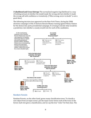
testing dataset will be used only once, in order to test the prediction model that
we've build on the training dataset. It is mandatory, as it is common to build a good
prediction model on a dataset (low in the sample error) but the same model
performs poorly on new data (out of sample error). This is known as over-fitting.
# set seed (in order all results to be fully reproducible) and create a
75-25 %
# partition for our data based on class variable
set.seed(1)
inTrain = createDataPartition(data1$classe, p = 3/4)[[1]]
# Assign the 75% of observations to training data
training1 = data1[inTrain,]
# Assign the remaining 25 % of observations to testing data
testing1 = data1[-inTrain,]
The fist prediction model was build by using the classification/Decision Trees
algorithm. In particular rpart method of the caret package was used in R. Then we
plotted the decision tree.
# Set seed (in order all results to be fully reproducible) and apply a
prediction
#Model with all variables
set.seed(1)
model.all <- train(classe ~ ., method="rpart", data = training1)
# Plot the Classification/Decision Tree
fancyRpartPlot(model.all$finalModel)
14. 13
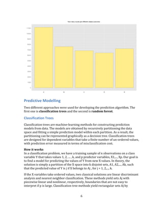
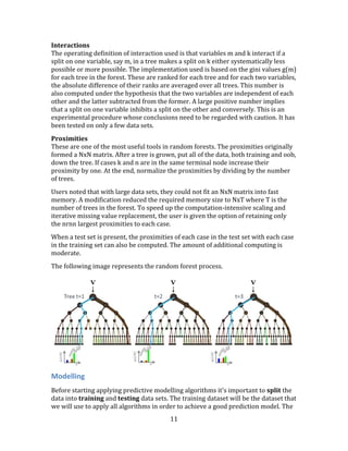
In order to check the accuracy rate of the model, we print the confusion Matrix. The
accuracy rate (around 50%) is low, so a further investigation is necessary. It is a
good idea to try a new algorithm on the training data.
# Apply the prediction
prediction <- predict(model.all, newdata= training1)
# Check the accuracy of the prediction model by printing the confusion
matrix.
print(confusionMatrix(prediction, training1$classe), digits=4)
## Confusion Matrix and Statistics
##
## Reference
## Prediction A B C D E
## A 7600 2375 2373 2122 762
## B 137 1898 156 893 740
## C 612 1422 2604 1809 1495
## D 0 0 0 0 0
## E 20 0 0 0 2414
##
## Overall Statistics
##
## Accuracy : 0.4932
## 95% CI : (0.4875, 0.4989)
## No Information Rate : 0.2844
## P-Value [Acc > NIR] : < 2.2e-16
15. 14
##
## Kappa : 0.3379
## Mcnemar's Test P-Value : NA
##
## Statistics by Class:
##
## Class: A Class: B Class: C Class: D Class: E
## Sensitivity 0.9081 0.33327 0.50731 0.0000 0.44613
## Specificity 0.6377 0.91886 0.78032 1.0000 0.99917
## Pos Pred Value 0.4989 0.49634 0.32788 NaN 0.99178
## Neg Pred Value 0.9458 0.85173 0.88232 0.8361 0.88899
## Prevalence 0.2844 0.19350 0.17440 0.1639 0.18385
## Detection Rate 0.2582 0.06449 0.08848 0.0000 0.08202
## Detection Prevalence 0.5175 0.12993 0.26984 0.0000 0.08270
## Balanced Accuracy 0.7729 0.62607 0.64381 0.5000 0.72265
Now we apply the random forest algorithm (with randomForest package in R) in
order to build our prediction model for the training dataset. The "in the sample
error" is almost 0%, which is great but it may indicates over-fitting. It is important
to check the out of sample error as well.
# Set seed (in order all results to be fully reproducible) and apply th
e random
# forest algorithm in the training dataset
set.seed(1)
modrf <- randomForest(classe ~. , data=training1)
# Create the prediction vector for the class in the training dataset
predictionsrf1 <- predict(modrf, training1, type = "class")
# Check the accuracy of the prediction model by printing the confusion
matrix.
confusionMatrix(predictionsrf1, training1$classe)
## Confusion Matrix and Statistics
##
## Reference
## Prediction A B C D E
## A 8369 0 0 0 0
## B 0 5695 0 0 0
## C 0 0 5133 0 0
## D 0 0 0 4824 0
## E 0 0 0 0 5411
##
## Overall Statistics
##
## Accuracy : 1
## 95% CI : (0.9999, 1)
## No Information Rate : 0.2844
## P-Value [Acc > NIR] : < 2.2e-16
16. 15
##
## Kappa : 1
## Mcnemar's Test P-Value : NA
##
## Statistics by Class:
##
## Class: A Class: B Class: C Class: D Class: E
## Sensitivity 1.0000 1.0000 1.0000 1.0000 1.0000
## Specificity 1.0000 1.0000 1.0000 1.0000 1.0000
## Pos Pred Value 1.0000 1.0000 1.0000 1.0000 1.0000
## Neg Pred Value 1.0000 1.0000 1.0000 1.0000 1.0000
## Prevalence 0.2844 0.1935 0.1744 0.1639 0.1838
## Detection Rate 0.2844 0.1935 0.1744 0.1639 0.1838
## Detection Prevalence 0.2844 0.1935 0.1744 0.1639 0.1838
## Balanced Accuracy 1.0000 1.0000 1.0000 1.0000 1.0000
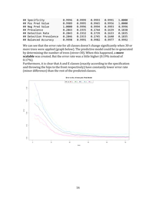
The average "out of sample error" is around 0.17%. The 95% confidence interval
for error rate is between 0.28% and 0.1%.
# Create the prediction vector for the class in the testing dataset
predictionsrf <- predict(modrf, testing1, type = "class")
# Check the accuracy of the prediction model by printing the confusion
matrix.
confusionMatrix(predictionsrf, testing1$classe)
## Confusion Matrix and Statistics
##
## Reference
## Prediction A B C D E
## A 2789 3 0 0 0
## B 0 1895 1 0 0
## C 0 0 1706 6 0
## D 0 0 4 1602 3
## E 0 0 0 0 1800
##
## Overall Statistics
##
## Accuracy : 0.9983
## 95% CI : (0.9972, 0.999)
## No Information Rate : 0.2843
## P-Value [Acc > NIR] : < 2.2e-16
##
## Kappa : 0.9978
## Mcnemar's Test P-Value : NA
##
## Statistics by Class:
##
## Class: A Class: B Class: C Class: D Class: E
## Sensitivity 1.0000 0.9984 0.9971 0.9963 0.9983
17. 16
## Specificity 0.9996 0.9999 0.9993 0.9991 1.0000
## Pos Pred Value 0.9989 0.9995 0.9965 0.9956 1.0000
## Neg Pred Value 1.0000 0.9996 0.9994 0.9993 0.9996
## Prevalence 0.2843 0.1935 0.1744 0.1639 0.1838
## Detection Rate 0.2843 0.1932 0.1739 0.1633 0.1835
## Detection Prevalence 0.2846 0.1933 0.1745 0.1640 0.1835
## Balanced Accuracy 0.9998 0.9991 0.9982 0.9977 0.9992
We can see that the error rate for all classes doesn't change significantly when 30 or
more trees were applied (graph below). The predictive model could be re-generated
by determining the number of trees (ntree=30). When this happened, a more
scalable was created. But the error rate was a little higher (0.19% instead of
0.17%).
Furthermore, it is clear that A and E classes (exactly according to the specification
and throwing the hips to the front respectively) have constantly lower error rate
(minor difference) than the rest of the predicted classes.
18. 17
Results & Conclusions
In Conclusion, after attempting with 2 different ways to build a model to predict the
the manner in which they did the exercise we concluded that the random forest
algorithm is the best one to use. This prediction model has an out of sample
error of 0.17% which is very good for our case. It is important here, to indicate that
the acceptability of the error rate depends on the problem itself.
For example, an error rate of 99.8% (just 0.2% accuracy rate) for a targeted on-line
advertisements campaign may be very good since the random accuracy rate is e.g.
0.1%. That will double the chances for a successful conversion.
On the other hand, an error rate of 99.9% may be unacceptable for predicting a
rare disease that actually occurs on 0.1% of the total population.
Furthermore, in our analysis, if we need a more scalable algorithm we have to
choose the 2nd random forest algorithm we created, which produces a little higher
error rate (0.19% versus 0.17%) but it is easier to produce and implement (only 30
trees were used).
19. 18
Bibliography
• Velloso, E.; Bulling, A.; Gellersen, H.; Ugulino, W.; Fuks, H. Qualitative Activity
Recognition of Weight Lifting Exercises. Proceedings of 4th International
Conference in Cooperation with SIGCHI (Augmented Human '13) . Stuttgart,
Germany: ACM SIGCHI, 2013. http://groupware.les.inf.puc-rio.br/har
• Qualitative Activity Recognition of Weight Lifting Exercises (source of original
dataset) http://groupware.les.inf.puc-
rio.br/static/WLE/WearableComputing_weight_lifting_exercises_biceps_curl_v
ariations.csv
• R Development Core Team, R: a language and environment for statistical
computing. R Foundation for Statistical Computing. http://www.r-project.org/
• Random forest package in R language http://cran.r-
project.org/web/packages/randomForest/index.html
• Caret package in R language http://cran.r-
project.org/web/packages/caret/index.html
• Forte Consultancy paper on predictive modelling
https://forteconsultancy.wordpress.com/2010/05/17/wondering-what-lies-
ahead-the-power-of-predictive-modeling/
• Classification and regression trees, by Wei-Yin Loh
http://www.stat.wisc.edu/~loh/treeprogs/guide/wires11.pdf
• Breiman, Leo, Jerome Friedman, R. Olshen and C. Stone (1984). Classification
and Regression Trees. Belmont, California: Wadsworth
• Mitchell, Tom M. (1997). Machine Learning. New York: McGraw-Hill
• Random Forests, Leo Breiman and Adele Cutler
https://www.stat.berkeley.edu/~breiman/RandomForests/cc_home.htm
• Huynh, Duy Tam Gilles Human Activity Recognition with Wearable Sensors,
PhD Thesis, Darmstadt, Germany.
• Decision Trees on Wikipedia
http://en.wikipedia.org/wiki/Decision_tree_learning
• Random Forests in Wikipedia http://en.wikipedia.org/wiki/Random_forest