This study used a machine learning technique called Generalized Factorization Method (GFM) combined with Non-negative Matrix Factorization (NMF) to analyze diffusion tensor imaging (DTI) data from 47 schizophrenia patients and 36 healthy controls. The goal was to determine if schizophrenia is a heterogeneous disorder with distinct patterns of white matter abnormalities. GFM identified 8 "biclusters" of schizophrenia patients that shared similar reductions in fractional anisotropy (FA) values in specific white matter regions. These biclusters mapped onto 4 general patterns of low FA, each associated with different clinical features. The study suggests schizophrenia comprises distinct subtypes that can be differentiated by white matter anomalies linked to symptom profiles.

1. Decomposition of brain diffusion imaging data uncovers latent
schizophrenias with distinct patterns of white matter anisotropy
Javier Arnedo a
, Daniel Mamah b
, David A. Baranger b
, Michael P. Harms b
, Deanna M. Barch b,c
,
Dragan M. Svrakic b
, Gabriel A. de Erausquin d
, C. Robert Cloninger b,e
, Igor Zwir a,b,
⁎
a
Department of Computer Science and Artificial Intelligence, University of Granada, Spain
b
Department of Psychiatry, Washington University School of Medicine, St. Louis, MO, USA
c
Department of Psychology and Department of Anatomy & Neurobiology Washington University, St. Louis, MO, USA
d
Roskamp Laboratory of Brain Development, Modulation and Repair, Department of Psychiatry and Behavioral Neurosciences (GAE), University of South Florida, Tampa, FL, USA
e
Department of Genetics (CRC), Washington University School of Medicine, St. Louis, MO, USA
a b s t r a c ta r t i c l e i n f o
Article history:
Received 9 December 2014
Accepted 28 June 2015
Available online 4 July 2015
Keywords:
Schizophrenias
White matter
Fractional anisotropy
Positive and negative symptoms
Biclusters
Generalized factorization
Non-negative Matrix Factorization
Model-based clustering
Consensus clustering
Fuzzy clustering
Possibilistic clustering
Relational clustering
Conceptual clustering
Fractional anisotropy (FA) analysis of diffusion tensor-images (DTI) has yielded inconsistent abnormalities in
schizophrenia (SZ). Inconsistencies may arise from averaging heterogeneous groups of patients. Here we inves-
tigate whether SZ is a heterogeneous group of disorders distinguished by distinct patterns of FA reductions. We
developed a Generalized Factorization Method (GFM) to identify biclusters (i.e., subsets of subjects associated
with a subset of particular characteristics, such as low FA in specific regions). GFM appropriately assembles a
collection of unsupervised techniques with Non-negative Matrix Factorization to generate biclusters, rather
than averaging across all subjects and all their characteristics. DTI tract-based spatial statistics images, which out-
put is the locally maximal FA projected onto the group white matter skeleton, were analyzed in 47 SZ and 36
healthy subjects, identifying 8 biclusters. The mean FA of the voxels of each bicluster was significantly different
from those of other SZ subjects or 36 healthy controls. The eight biclusters were organized into four more general
patterns of low FA in specific regions: 1) genu of corpus callosum (GCC), 2) fornix (FX) + external capsule (EC),
3) splenium of CC (SCC) + retrolenticular limb (RLIC) + posterior limb (PLIC) of the internal capsule, and 4) an-
terior limb of the internal capsule. These patterns were significantly associated with particular clinical features:
Pattern 1 (GCC) with bizarre behavior, pattern 2 (FX + EC) with prominent delusions, and pattern 3
(SCC + RLIC + PLIC) with negative symptoms including disorganized speech. The uncovered patterns suggest
that SZ is a heterogeneous group of disorders that can be distinguished by different patterns of FA reductions
associated with distinct clinical features.
© 2015 Elsevier Inc. All rights reserved.
Introduction
White matter lesions in the brain are generally associated with ab-
normal connectivity of brain regions in complex diseases such as schizo-
phrenia (SZ) (Lee et al., 2013; Liu et al., 2013; Skudlarski et al., 2013). It
has been reported that white matter abnormalities may suggest clues
relevant to the neurodevelopmental origin of these diseases (Huang
et al., 2011; Keller et al., 2007; Lee et al., 2013). To allow the investiga-
tion of white matter structural abnormalities in vivo, diffusion tensor
imaging (DTI) has been widely used; this magnetic resonance imaging
technique measures localized water diffusivity reflecting the geometric
properties and directionality of both the axonal membrane and myelin
in large white matter tracts of the brain (Mori, 2007). Fractional
anisotropy (FA) is a scalar measure often used in DTI, which describes
the directional dependence of diffusion (i.e., anisotropy); it is related
to axonal fiber density, axonal diameter and myelination in white
matter (Mori, 2007; Song et al., 2002). Unfortunately, DTI findings
in SZ have been inconsistent across studies (Alba-Ferrara and de
Erausquin, 2013; Kubicki et al., 2007). Specifically, studies have either
reported no white matter FA differences between controls and patients
with SZ (Foong et al., 2002; Suddath et al., 1990; Wible et al., 1995),
minimal regional FA abnormalities (Lee et al., 2013; Liu et al., 2013;
Skudlarski et al., 2013), or widespread FA abnormalities (Douaud
et al., 2007; Lim et al., 1999; Minami et al., 2003).
The inconsistencies in SZ studies may arise from averaging heteroge-
neous groups of patients with varying FA abnormalities (Fig. 1). Identi-
fication of relevant changes in FA is particularly challenging when
subjects vary extensively in their clinical features and severity, which
are likely to have complex relations with different brain structures
and functions (Blanchard and Cohen, 2006; Holliday et al., 2009).
Regional differences can be missed due to the fuzziness of the data,
NeuroImage 120 (2015) 43–54
⁎ Corresponding author at: Washington University School of Medicine, Barnes-Jewish
Hospital (south), Renard Building 4940 Children's Place, Room 2202, Campus Box 8134,
St. Louis, MO 63110, USA.
E-mail address: zwiri@psychiatry.wustl.edu (I. Zwir).
http://dx.doi.org/10.1016/j.neuroimage.2015.06.083
1053-8119/© 2015 Elsevier Inc. All rights reserved.
Contents lists available at ScienceDirect
NeuroImage
journal homepage: www.elsevier.com/locate/ynimg

2. particularly when the abnormality is mild (Alba-Ferrara and de
Erausquin, 2013).
To characterize the heterogeneity of structural brain abnormalities in
SZ, we devised an unsupervised machine learning approach that decom-
poses a collection of FA images from patients with SZ into local partitions
or biclusters (Cichocki, 2009; Pascual-Montano et al., 2006b; Tamayo
et al., 2007). These biclusters are composed of co-differentiated white
matter FA sets of voxels (i.e., voxels with low FA values) shared by
subsets of subjects. Biclustering captures local and intrinsic relationships
between subsets of observations (subjects) sharing subsets of descrip-
tive features (voxels) instead of relationships between all subjects and
all their descriptive features. These relationships can be weakened
when all features are used in a single global model of data, as is typically
done by clustering methods.
Our approach combines the advantages of a number of complemen-
tary clustering strategies into a Generalized Factorization Method (GFM,
Supplementary Fig. 1) and has been previously widely applied in differ-
ent biomedical problems (Harari et al., 2010; Romero-Zaliz et al., 2008b;
Zwir et al., 2005b). Non-negative Matrix Factorization (NMF) algo-
rithms have also been utilized in facial recognition (Lee and Seung,
1999), gene expression (Tamayo et al., 2007), and several other bio-
medical problems (Cichocki, 2009). More recently, we successfully
applied a composite GFM–NMF to uncover eight different subtypes of
SZ by dissecting genome wide association studies into biclusters com-
posed of distinct sets of genetic variants and clinical symptoms of SZ
patients (Arnedo et al., 2013, 2014).
In the current study, we applied the GFM–NMF methodology to
examine a sample of SZ patients and healthy controls whose
diffusion-weighted brain images were processed using Tract Based
Spatial Statistics (TBSS) (Smith et al., 2006). We refer to the output
of TBSS, which is the locally maximal FA projected onto the group
white matter skeleton, as an FA-TBSS image. We searched for
biclusters reflecting different FA patterns that can be shared by dis-
tinct subsets of SZ patients. Then we evaluated the significance of
each bicluster by comparing the differential FA within a bicluster
with that exhibited by healthy controls, as well as with that shown
in other individuals with SZ who were not present in the bicluster.
We then analyzed the anatomical location of DTI abnormalities iden-
tified in the biclusters. In the final step, we cross-correlated the un-
covered biclusters with collected descriptions of clinical features of
the patients including positive and negative symptoms scores as de-
fined by the Scale for the Assessment of Positive Symptoms (SAPS)
and the Scale for the Assessment of Negative Symptoms (SANS)
(Andreasen, 1984).
The method illustrated here is able to agnostically decompose FA-
TBSS images and to distinguish subsets of SZ patients using white
matter FA patterns, just as we decomposed SZ into subtypes with com-
plex relations between sets of genotypes and sets of clinical phenotypes
(Arnedo et al., 2014). These abnormalities may suggest distinct etiolo-
gies in patients diagnosed with SZ, characterized by different brain
areas leading to distinct symptoms and clinical outcomes. The software
is available upon request from the authors.
a) b)
c) d)
Fig. 1. Synthetic example of global and local tensor identification in patients. (a) Synthetic 2nd order tensor representation of TBSS images (i.e., x and y dimensions from subjects with
different local abnormalities. (b) Voxelgrams corresponding to a 3rd order tensor representation of TBSS images in (a) (i.e., x, y, and subject dimensions). (c) Averaged values of all tensors
in (a). (d) Voxelgram corresponding to (c).
44 J. Arnedo et al. / NeuroImage 120 (2015) 43–54

3. Methods
Study sample
The participants included in the study were drawn from a popula-
tion of volunteers for studies of brain structure and function at the
Conte Center for the Neuroscience of Mental Disorders at Washington
University Medical School, St. Louis. All participants gave written
informed consent for participation following a complete description of
the risks and benefits of the study.
Participants consisted of 47 individuals (mean age = 37.2 yrs; SD =
8.5) who met DSM-IV (American_Psychiatric_Association, 1994)
criteria for SZ, and outpatients at the time of study. Diagnosis was
ascertained by consensus between a research psychiatrist, who con-
ducted a semi-structured interview, and a trained research assistant
who used the Structured Clinical Interview for DSM-IV Axis I Disorders
(First et al., 2002). Participants were excluded if they: (1) met DSM-IV
criteria for substance abuse or dependence within the past 6 months;
(2) had a clinically unstable or severe medical condition, or a medical
condition that would confound the assessment of psychiatric diagnosis
(e.g., hypothyroidism); (3) had a history of head injury with neurolog-
ical sequelae or loss of consciousness; or (4) met DSM-IV criteria for
mental retardation (mild or greater in severity). Participants include
16 females and 31 males. Ethnically, they included 1 Asian, 26 Blacks/
African Americans, 19 Caucasians, and 1 multiracial. Five participants
were left handed, and the rest were right handed.
Control participants consisted of 36 individuals (mean age =
36.9 yrs; SD = 9.1) who did not meet criteria for DSM-IV schizophrenia,
bipolar disorder, or major depression. Other exclusion criteria were the
same as for the SZ subjects. Control participants included 19 females
and 17 males. Ethnically, they included 24 Blacks/African Americans
and 12 Caucasians. Two control participants were left handed, and 34
were right handed.
Clinical measures
The presence and severity of positive (psychotic) symptoms was
assessed using the Scale for the Assessment of Positive Symptoms
(SAPS)(Andreasen, 1984). Negative symptoms were assessed using the
Scale for the Assessment of Negative Symptoms (SANS) (Andreasen,
1984).
Image acquisition and pre-processing
Magnetic resonance (MR) scans were obtained using a 3 T Siemens
Tim Trio scanner with a 12-channel head coil. Structural images were
acquired using a sagittal magnetization-prepared radiofrequency rapid
gradient-echo 3D T1-weighted sequence (TR = 2400 ms, TE =
3.16 ms, flip angle = 8°, voxel size = 1 mm isotropic). Two DTI scans
(each ~ 5 min) were acquired in an oblique–axial plane with a single
shot echo-planar imaging (EPI) sequence with TR = 8000 ms, TE =
86 ms, FOV 224 × 224 mm2
, 2 mm isotropic voxels (112 matrix with
64 slices of 2 mm), phase encoding in the A–P direction, 6/8 partial
Fourier, and a parallel acceleration factor in the phase direction of 2
(GRAPPA = 2). Each DTI scan consisted of 30 volumes acquired
with non-collinear diffusion-sensitizing directions at a b-value of
800 s/mm2
and five interspersed volumes acquired without diffusion
weighting (b-value = 0 s/mm2
).
Data from the two DTI scans was concatenated and then pre-
processed using FMRIB Software Library (FSL) version 4.1 (Nacsa et al.,
2004). Briefly, within a given subject, a reference b = 0 volume was
brain-extracted (Smith, 2002) and the diffusion-weighted volumes
were registered to this reference to correct for movement and eddy
current distortion (using FSL's ‘eddy_correct’). A diffusion tensor was
derived at each voxel using a standard least-squares fitting (FSL's ‘dtifit’)
to provide voxel-wise calculations of fractional anisotropy (FA). As a
quality control mechanism, the residual error between the calculated
tensor model fit and original data was computed for each slice and vol-
ume. Volumes containing slices with poor model fits were removed
from the data, and the diffusion tensor and FA were recomputed with-
out the problematic volumes. This is an effective mechanism to identify
and remove volumes with artifacts due to motion or other scanner
anomalies (e.g., signal loss due to the table vibration artifact discussed
in Gallichan et al. (2010).
DTI data analysis: Tract Based Spatial Statistics (TBSS)
TBSS was carried out using FSL 4.1 (Smith et al., 2006). All partici-
pants' FA data were projected onto a mean FA image using the non-
linear registration tool FNIRT to register to the FMRIB58_FA standard
brain template. The registered data was thinned to create a mean FA
skeleton restricted to voxels with the highest FA at the center of the
major WM tracts. Following visual assessment of the optimal threshold
value, the skeleton was thresholded at the recommended level of FA =
0.2 in order to remove confounding low-FA voxels, which may be caused
by partial volume effects of gray matter or cerebrospinal fluid. Each
participant's aligned FA data were projected onto the skeleton by searching
the maximum FA value in a region perpendicular to the skeleton (FA-TBSS
image). This projection was performed for every subject.
Rationale of the Generalized Factorization Method (GFM) and the Non-
negative Matrix Factorization method (NMF)
Our GFM was designed and successfully applied to identify structur-
al patterns or clusters (substructures) that characterize complex objects
embedded in databases (Cordon et al., 2002; Romero-Zaliz et al., 2008a;
Ruspini and Zwir, 2002; Zwir et al., 2005a). Unfortunately, solving these
kinds of complex problems cannot be resolved by a single clustering
method but only by utilizing and combining the advantages of many
of them, as we implemented in GFM and summarized below (Supple-
mentary Fig. 1, see Supplementary Methods). NMF algorithms find an
approximate factoring of the data: M ~ WK × HK, where both decompo-
sition matrices have only positive entries (Arnedo et al., 2013; Lee and
Seung, 1999; Pascual-Montano et al., 2006b; Tamayo et al., 2007) (see
Supplementary methods). WK is an n × K matrix that defines the sub-
matrix decomposition model whose columns specify how much each
of the subjects contributes to each of the k sub-matrices. HK is a k × m
matrix whose entries represent the FA values in the k sub-matrices for
each of the m voxels. Biclusters composed of distinct subsets of
features/attributes shared by subsets of observations are derived from
each sub-matrix. We integrated the GFM and NMF (GMF–NMF) to
identify biclusters that can handle sparse, fuzzy and different data
granularity (Cichocki, 2009).
The GFM–NMF method: identifying biclusters in FA-TBSS images
This method distinguishes four main processes (Fig. 2) where FA-
TBSS images from different subjects were appropriately encoded, and
multiple biclusters were determined and evaluated based on quality
measures (sensitivity, generality) to select an optimal descriptive set.
During selection, niches (group of observations of sufficient similarity
in the search space) are defined to run selection locally and provide di-
verse but still optimal biclusters. Finally, biclusters were topologically
organized and decoded into NIfTI 3D images.
Codification of the image database
Flattening each subject's FA-TBSS image produced a vector (e.g.
[voxels × subject], Fig. 2) (Cichocki, 2009). These vectors were included
as rows in matrix M using oro.nifti package, R version 2.15.1, where each
row corresponded to a subject and each column to a tagged voxel
(e.g., voxel_ID). Here, 126,586 voxels were present in the TBSS skeleton,
and those cells corresponding to voxels outside the TBSS skeleton were
45J. Arnedo et al. / NeuroImage 120 (2015) 43–54

4. removed from the matrix. The tagging order was used for posterior
reconstruction of the images (see step 4). (Note that the coordinates
(x, y, z) of the voxels in the RX × Y × Z
space are not necessary for the
comparison of their FA values and for reconstructing images from
matrices in this particular problem.) For convenience, we utilized trans-
posed (MT
) and normalize matrix M by scaling each column in the [0, 1]
interval Eq. (1):
a0
x;y;z ¼ 1−
ax;y;z−Min ax;:;z
À Á
Max ax;:;z
À Á
−Min ax;:;z
À Á ; ∀ax;y;z∈M: ð1Þ
Here the assumption is that we were interested in identifying voxels
with low values relative to the rest of the patients rather than in finding
voxels with the global lowest FA values. Therefore, we reversed the
ordering so that low FA values produced entries near 1. This approach
facilitates the search of biclusters by NMF methods, which tend to
favor groupings of high values.
Factorization of the image database
Decomposition of the matrix M into sub-matrices Mk = 1, …, K using the
Fuzzy NMF (NMF) implementation of the NMF method with default
Fig. 2. The GFM–NMF method: identifying biclusters in FA-TBSS images. The method consists of four main steps: (1) codification of the image database; (2) factorization of the image
database; (3) optimization and organization of the factorized image database; and (4) folding the optimal biclusters into NIfTI 3D images for visualization.
46 J. Arnedo et al. / NeuroImage 120 (2015) 43–54

5. parameters as described in Arnedo et al. (2013), where K corresponds to the
maximum numbers of possible sub-matrices (i.e., clusters). For K = 2 to
√ n, where n is the number of subjects in the sample, apply FNMF to M
recurrently and calculate the corresponding HK and WK matrices. 40 dif-
ferent initializations of the FNMF parameters were run before selecting
the best results for a given K (see Sampling in Supplementary methods),
which are normally enough runs to achieve internally robust sub-
matrices (Arnedo et al., 2013; Pascual-Montano et al., 2006a,b).
Identification of biclusters from FNMF factorizations. Select the most rep-
resentative columns and rows in the HK and WK matrices, respectively,
for each one of the k-factors (sub-matrices) independently. Sorting
the rows in WK for each column in descending order and selecting
those rows that are higher than a given threshold achieves this (see
below). Analogously, repeat the process for the HK matrix to select the
columns. The set of selected rows (voxels) and columns (subjects) for
each factor define a bicluster Bk, with k = [1, …, K].
The threshold (Eq. (2)) for factor k in the matrix HK is defined in the
unit interval [0–1] and calculated as:
Threshold ¼ max Hkð Þ Ã 1−δð Þ ð2Þ
with δ being the degree of fuzzinesss of the bicluster (same criterion
was used for selecting rows in W_K). Here, a default δ = 0.35 was uti-
lized, which is consistent with the typical 70–30% ± 5% partition of
the holdout (2-fold crossvalidation) sampling method (Mitchell,
1997) (see sensitivity analysis of this parameter in Supplementary
methods).
Elimination of redundant biclusters. Because FNMF identifies biclusters in
partitions with different number of clusters K, it is possible that the
same bicluster can be generated more than one time. Biclusters with a
high degree of overlap are considered once. The degree of overlap
between two biclusters was assessed by calculating the pairwise proba-
bility of intersection among them based on the hypergeometric distri-
bution (PIhyp, Eq. (3)) (Tavazoie et al., 1999; Zwir et al., 2005a):
PIhyp Bi; Bj
À Á
¼ 1−
Xp−1
q¼0
h
q
g−h
n−q
=
g
h
; h ¼ Bij j; n ¼ Bj
; p
¼ Bi∩Bj ð3Þ
where p observations(subjects)/features(voxels) belong to bicluster Bi
with size h, and also belong to a bicluster Bj of size n; and g is the total
number of observations. Therefore, the lower the PIhyp, the higher the
overlapping and the better co-cluster coincidence. Here, a default
PIhyp b 1E−03 was utilized (Arnedo et al., 2013; Tavazoie et al., 1999;
Zwir et al., 2005b). Biclusters harboring b10% of the total number of
subjects were not considered to avoid a trend to obtain singleton
biclusters.
Optimization and organization of the factorized image database
Evaluation of biclusters. Biclusters were characterized by two objectives:
specificity and generality. Specificity is defined as the frequency
of voxels displaying low FA values in a bicluster relative to the entire
FA-TBSS image (Eq. (4)):
Specificity Bið Þ ¼
# voxels ∈Bi
# total voxels
ð4Þ
where voxels in Bi correspond a subset of low FA values (Eq. (1)) shared
by a particular subset of subjects, and total voxels correspond to the
entire voxels in an FA-TBSS image (Eq. (4)). Here the assumption is
that our data are sparse, and thus, large number of voxels may produce
associations with diverse brain regions (suggesting low specificity),
whereas a small number of voxels tend to be concentrated in a single
or a few cohesive locations (suggesting high specificity) (Arnedo et al.,
2014; Cordon et al., 2002; Ruspini and Zwir, 2002; Zwir et al., 2005a).
Generality is defined in the same fashion but with respect to the
subjects in a bicluster (Eq. (5)):
Generality Bið Þ ¼
# subjects ∈Bi
# total subjects
ð5Þ
where subjects in Bi share particular subsets of voxels with low FA
values. Here the assumption is that biclusters generated with a small
maximum number of clusters K (low granularity) tend to include a
large number of subjects, and thus, they are likely to share a more
heterogeneous set of features (voxels with low FA values) than a small-
er group of subjects from a bicluster generated when using a large K
value (high granularity) (Arnedo et al., 2014; Cordon et al., 2002;
Ruspini and Zwir, 2002; Zwir et al., 2005a, see sensitivity analysis of
parameters in Supplementary methods).
Another indirect objective considered for the evaluation of biclusters
is the generation of diverse patterns that completely describe objects
(patients). Therefore, our approach evaluates the specificity and gener-
ality objectives described above in a local niche (Deb, 2001a,b; Ruspini
and Zwir, 2002; Zwir et al., 2005a). Both specificity and generality
measurements are based on counting objects within a bicluster without
distinguishing among them (e.g., # subjects). However, diversity differ-
entiates which objects are within a bicluster, and thus, biclusters
harboring distinct objects are allocated in different niches. These niches
are calculated using Jaccard's metric between biclusters (Romero-Zaliz
et al., 2008a,b) (i.e., inclusion of subjects, Eq. (6)):
Niching Bi; Bj
À Á
¼
S Bið Þ ∩S Bj
À Á
S Bið Þ ∪S Bj
À Á Nγ ð6Þ
where Bi and Bj were the two different biclusters, the S functional re-
trieves the subjects in the biclusters in a particular niche, and γ (0.7 or
70%) is size of the niche determined by the degree of overlapping/inter-
section between biclusters. Here the assumption is that the niches are
equivalence classes dictated by the degree of overlapping/inclusion
between subjects in the biclusters.
Selection of optimal biclusters using multiobjective and multimodal optimi-
zation techniques. Optimal biclusters were obtained as a tradeoff
between two opposing objectives: sensitivity and generality (Arnedo
et al., 2014; Deb, 2001a,b; Ruspini and Zwir, 2002; Zwir et al., 2005a).
A Pareto-optimization strategy searches for solutions that are non-
dominated in the sense that there was no other solution superior in all
objectives being selected (i.e., close to Minimum Description-Length
(MDL) (Rissanen, 1989)). The dominance relationship as a minimiza-
tion problem is defined as (Eq. (7)):
a≺b if f ∀i Oi að Þ≤Oi bð Þ ∃j Oj að Þ≤Oj bð Þ ð7Þ
where the Oi and Oj are either specificity or generality objectives.
Optimization of small sets of biclusters was exhaustively implemented,
whereas evaluation of large sets is approached by genetic algorithms, as
described in Harari et al. (2010) and Romero-Zaliz et al. (2008a,b).
MDL-like optimization approaches recommend the “best” model by op-
timizing the sum of the model accuracy and its size (single objective),
and encode the information into bits. Pareto-based optimization solves
the original multi-objective problem by treating the model-quality
criteria of accuracy and size as two separate quality measures, and is
more generic than MDL since it can cope with any kind of non-
commensurable model-quality criteria (Freitas, 2004; Ruspini and
Zwir, 2002; Zwir et al., 2005a).
Our approach applied the non-dominance relationship described
above locally. That is, it identifies all non-dominated optimal
biclusters that have no better solution (i.e., multiobjective) in a
47J. Arnedo et al. / NeuroImage 120 (2015) 43–54

6. niche (i.e., multimodality) or equivalence class defined based on the
non-dominance partial order (Deb, 2001a; Ruspini and Zwir, 2002;
Zwir et al., 2005a). Then, given two biclusters where one of them has
the same or even worst sensitivity and generality than the other but
correspond to different sets of subjects, both biclusters will be pre-
served because they are in different niches. Biclusters containing b10%
of the total number of subjects were not considered to avoid a trend
yielding singleton biclusters. Statistical significance was used as an in-
dependent validation measurement of the bicluster quality (see below).
Topological organization of optimal biclusters into hierarchies. Non-
dominated biclusters in each niche were top-down organized into
hierarchies (networks or sub-graphs) from the most general (i.e., the
bicluster containing the greatest number of subjects, see above) to the
most specific (i.e., the bicluster containing the smallest and most
cohesive set of voxels, as described above). Note that one bicluster can
belong to more than one niche based on the Niching function described
above, or hierarchies can be disjoint when mapping to independent sets
of subjects. Biclusters are renamed as Bi,j, where i corresponds to a par-
ticular hierarchy, and j to the order in such hierarchy (smallest j-value
indicates the most general and top level bicluster).
Folding the optimal biclusters into NIfTI 3D images for visualization
A new NIfTI 3D image was generated for each bicluster from its
corresponding matrix representation to visualize the location of specific
FA voxels on the FA-TBSS images using the oro.nifti package in R version
2.15.1. The tagging order (voxel_ID, see step (1)) used for encoding
FA-TBSS images was utilized in a reverse fashion.
Sensitivity analysis of parameters
Comparisons between algorithms (i.e., the bioNMF and the FNMF
biclustering methods) and evaluation of parameters, including initiali-
zation and stopping criteria, outlier detection, number of clusters, and
degree of fuzziness in the NMF methods are described in Supplementa-
ry Methods.
Sampling analysis
Sampling analysis was performed by leave-one-out and leave-one-
bicluster-out as described in Supplementary methods.
Statistical analysis
Statistical analysis was performed by using one-way ANOVA,
pairwise t-test and Bonferroni correction (R version 2.15.1) as described
in Supplementary methods.
Statistical analysis
Identification of biclusters was unbiased without a prior knowledge
of the anatomical location of voxels and/or the clinical symptoms of the
subjects. Using internal criteria in cluster evaluation is biased towards
algorithms that use the same cluster model (Bezdek, 1998). Therefore,
external evaluations based on criteria that were not used for clustering,
such as tests based on ANOVA and its F-statistic, are often added to the
cluster evaluation (Färber et al., 2010). To assess the statistical signifi-
cance of the findings, we compared the average FA in the set of voxels
of each bicluster with the average FA value in the same voxels of either
SZ subjects who were not included in the bicluster or healthy controls
by one-way ANOVA and pairwise t-test (R version 2.15.1) and applying
Bonferroni correction. Evaluation of global differences in FA between all
patients and all controls has been performed in the same fashion. One
factor ANOVA using GLM-univariate was used to test the interactions
of FA reduction and gender in each hierarchy by creating a new two-
level variable named “interact” (voxels × proportion of gender in a
bicluster). (Hierarchies were utilized to account for a larger number of
observations.) The obtained results cannot reject the null hypothesis
of a different proportion of a particular gender than that of the original
sample in each hierarchy (p-value N 0.1, after correction for multiple
test, B1,1 was omitted since it has only 5 members).
Results
Biclusters encode sets of voxels with FA reductions shared by subsets of
subjects with SZ
We first investigated decreased FA regions in a sample composed of
TBSS images from 47 SZ patients, which together did not exhibit signif-
icant differences from a similar sample composed of 36 images of
healthy controls (see Statistical analysis, Methods, p-value N 0.81). A
partition of the images corresponding to the patients with SZ using
GFM–NMF uncovered eight optimal local partitions or biclusters,
where each bicluster encoded a subset of subjects characterized by a
similar degree of FA reduction in a particular subset of voxels. This
method allowed any given subject and/or voxel to belong to more
than one bicluster or to none of them (see Methods). The mean FA of
the voxels in each of the eight biclusters significantly differed from the
mean FA for voxels in the same location in either the other SZ subjects
not included in that bicluster or from the healthy controls after correc-
tion for multiple comparisons (see Statistical analysis, Methods,
Table 1, Figs. 3–4). This suggests that the biclusters should separately
explain a large part of the variability in the population. In fact, 41 of
the 47 SZ subjects were included in at least one bicluster (Table 1),
which accounted for N95% of the FA variance across subjects (in the
population) and suggests a high degree of generality.
The biclusters varied in terms of their size, based on the associated
numbers of subjects and shared voxels. For example, one general
bicluster (i.e., one having high coverage) contained 21 subjects and
9744 voxels, while another specific bicluster (i.e., one having low cover-
age) contained only 5 subjects and 1322 voxels. While generality
implies a large coverage of the sample; specificity displays smaller but
more cohesively arranged and shared sets of FA voxels in the sample.
The latter two biclusters did not overlap, and thus were associated
with FA reductions in different brain regions, as expected. On the
other hand, another pair of biclusters containing 15 subjects with
5147 voxels and 5 subjects with 2637 voxels respectively, showed a
high degree of overlap, describing FA reductions in similar brain regions
but with distinct degrees of specificity and generality (Fuzzy clustering
(Bezdek, 1981)). These results suggests that the biclusters uncovered by
GFM vary and are optimal in terms of their specificity and generality, as
well as diversity, which is exemplified by the brain region described by
them (see Methods).
Topological organization of biclusters uncovers functionally meaningful
local regions of FA reduction
Because the identification of biclusters is not constrained by
predefined knowledge about the anatomical region of the voxels, any
grouping strategy may eventually identify sets of subjects sharing low
FA values in voxels scattered throughout the whole brain. To evaluate
the biological meaningfulness of FA reduction regions uncovered in
the biclusters, our method topologically organized the eight biclusters
into four main equivalence classes. The equivalence classes are defined
by the partial order imposed by the non-dominance relationship among
biclusters, that is, there is no better solution in both sensitivity and
generality within each class (see Methods). Although “equivalent”,
optimal biclusters within (and eventually across) these classes can be
ordered on the basis of the inclusion of their subjects (Jech, 2003;
Romero-Zaliz et al., 2008a; Zwir et al., 2005a,b) (see Methods, Table 1,
and Supplementary Fig. 2). This organization of the classes is termed
hierarchies, where biclusters located at the top and at the bottom of a
48 J. Arnedo et al. / NeuroImage 120 (2015) 43–54

7. hierarchy correspond to the most general and to the most specific
biclusters, respectively. Moreover, all biclusters in a hierarchy are opti-
mal in the sense that one bicluster is not worse (i.e., dominated) than
another in both the objectives of specificity and generality (i.e., see
multiobjective/multimodal optimization (Deb, 2001a,b; Zwir et al.,
2005a,b), Methods, Table 1). Disjoint hierarchies indicate diversity of
biclusters, and thus provide a distributed coverage and description of
the sample.
Re-mapping of FA reduction regions from biclusters onto the
original TBSS images, revealed that voxels with decreased FA tended
not to be scattered but to be confined to certain areas for each hier-
archy, and were localized to white matter tracts potentially relevant
to the pathophysiology of SZ (Fig. 5). The four identified hierarchies
mapped to different anatomical regions (see Fig. 1 in Huang et al.,
2011), Fig. 5).
The first hierarchy involved only one bicluster with decreased FA
primarily in the genu of the corpus callosum (GCC) (Table 1, Fig. 5a).
The second hierarchy included biclusters with patients involving FA
reductions primarily in the fornix (FX) and/or in the external capsule
(EC) (Table 1, Fig. 5b). The most general bicluster in this hierarchy
included patients with FA reduction in both FX and EC, whereas another
more specific bicluster in the same hierarchy differentiated a subset of
patients with FA reduction only in the FX. The third hierarchy included
biclusters with FA reductions in the retrolenticular limb of internal
Table 1
Hierarchies containing biclusters uncovered by the GFM–NMF and their statistical significance (biclusters in bold are specifically illustrated in Fig. 5, and all biclusters are hierarchically
shown in Supplementary Fig. 2).
Hierarchies⁎1/biclusters #Subjects #Voxels Anatomical location ANOVA F-test*2
Multiple comparison T-test*3
Controls Rest of patients
B1,1 5 1322 GCC 4.07E−04 5.40E−04 2.90E−04
B2,1 15 5147 FX, EC 1.17E−07 7.20E−05 5.40E−08
B2,2 7 3379 FX 2.63E−05 1.80E−04 1.40E−05
B2,3 5 2637 FX 1.92E−03 4.90E−03 1.30E−03
B3,14,1 21 9744 ALIC, PLIC 5.89E−09 1.50E−04 2.50E−09
B3,2 9 2569 SCC, PLIC, RLIC 1.13E−07 1.50E−05 5.20E−08
B3,3 6 974 SCC, PLIC, RLIC 7.05E−04 2.89E−03 4.40E−04
B4,2 11 1200 ALIC 1.01E−04 6.70E−04 6.80E−05
*1
Bi,j indicates bicluster j in the hierarchy i.
*2
F-test corresponds to the p-value derived from the cdf of F-statistic in the one-way ANOVA (R version 2.15.1, aov()).
*3
T-test corresponds to the p-value derived from pairwise comparisons of means by T-test corrected by Bonferroni (R version 2.15.1, pairwise.t.test()).
a) b)
c) d)
Fig. 3. Comparison of average FA values of four different biclusters. Box plots depict average FA values of four biclusters compared to identically located FA voxel values in SZ subjects who
were not included in each specific bicluster and in healthy controls. Calculations were performed by one-way ANOVA (R version 2.15.1, function aov(), Table 1). Biclusters are renamed as
Bi,j, where i corresponds to a particular hierarchy, and j to the order in such hierarchy (smallest j-value indicates the most general and top level bicluster). (a) Comparisons for bicluster B1,1.
(b) Comparisons for bicluster B2,3. (c) Comparisons for bicluster B3,3. (d) Comparisons for bicluster B4,2.
49J. Arnedo et al. / NeuroImage 120 (2015) 43–54

8. capsule (RLIC), and/or in the posterior limb of internal capsule (PLIC),
and/or in the splenium of the corpus callosum (SCC) (Table 1, Fig. 5c).
Remarkably, the FA reduction in the SCC was not prominent in the
most general bicluster of 21 subjects within this hierarchy; however,
the FA reduction in the SCC was prominent in a more specific bicluster
within the larger group of subjects. The fourth hierarchy partially
overlapped with the third, and shared their most general bicluster
(Supplementary Fig. 2). Despite this overlap, the most specific bicluster
in the fourth hierarchy was different from the rest of the patients and
the other biclusters (Table 1, Figs. 3–4), showing FA reductions in the
anterior limb of internal capsule (ALIC, Fig. 5d).
Post hoc analysis of the subjects identified by disjoint biclusters uncovers
distinct subsets of SZ patients with slightly different phenotypes
To evaluate associations of each hierarchy's FA reductions with clinical
features, we analyzed scores of SAPS and SANS items and domains (Sup-
plementary Table 1, Fig. 6). Subjects within the first hierarchy were more
likely to have certain bizarre behavior symptoms (i.e., social–sexual be-
havior, aggressive behavior), certain formal thought disorder symptoms
(i.e., derailment and pressured or distractible speech), and delusions of
reference (Supplementary Table 1, Fig. 6). These symptoms were
b)
c)
d)
a)
Fig. 4. Expanded comparison of average FA values of the four different biclusters described
in Fig. 3. Box plots depict average FA values of four biclusters compared to identically lo-
cated FA voxel values in all other SZ subjects, SZ subjects in the other biclusters, and
healthy controls. Calculations were performed using one-way ANOVA (R version 2.15.1,
function aov()). Biclusters are renamed as Bi,j, where i corresponds to a particular hierar-
chy, and j to the order in such hierarchy (smallest j-value indicates the most general
and top level bicluster). (a) Comparisons for bicluster B1,1 (ANOVA p-value b 1.39E−03).
03). (b) Comparisons for bicluster B2,3 (ANOVA p-value b 1.50E−03). (c) Comparisons
for bicluster B3,3 (ANOVA p-value b 1.42E−04). (d) Comparisons for bicluster B4,2
(ANOVA p-value b 7.48E−06). Remarkably, the average FA values of biclusters B1,1 and
B2,3 are higher – instead of lower – than the TBSS mean exhibited by the controls and
the rest of the patients when voxels of the fourth (d) bicluster are evaluated.
a)
b)
c)
d)
Fig. 5. Representation of low FA regions in white matter for different biclusters.
Figures depict axial, sagittal, and coronal slice representations (left to right panels) of
four biclusters mapping specific structural abnormalities (i.e., low FA), to regions on the
brain white matter tracts. The utilized convention is that the right side corresponds to
the right of the image. Gray pixels represent voxels included in the TBSS skeleton. Red
pixels represent voxels from the TBSS skeleton that were identified by the corresponding
biclusters (see Table 1). Biclusters are renamed as Bi,j, where i corresponds to a particular
hierarchy, and j to the order in such hierarchy (smallest j-value indicates the most general
and top level bicluster). (a) Representation of Bicluster B1,1. (b) Representation of Bicluster
B2,3. (c) Representation of Bicluster B3,3. (d) Representation of Bicluster B4,2.
50 J. Arnedo et al. / NeuroImage 120 (2015) 43–54

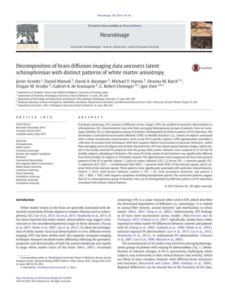
9. Fig. 6. Clinical relationships of biclusters. The bar plots show the averaged severity of positive (psychotic) symptoms (SAPS and SANS scales) for subjects included in bicluster B1,1 (blue bars), bicluster B2,3 (red bars), bicluster B3,3 (green bars), bicluster
B4,2 (purple bars), and the rest of the patient sample (light blue bars). Biclusters are renamed as Bi,j, where i corresponds to a particular hierarchy, and j to the order in such hierarchy (smallest j-value indicates the most general and top level bicluster).
Significant differences in means of items exhibited by subjects of a particular bicluster are indicated with an asterisk (detailed statistics are indicated in Supplementary Table 1). Three sets of symptoms were linked with particular biclusters: delusion,
bizarre behavior, and affective flattening or alogia symptoms were associated primarily with bicluster B2,3 (red brace), bicluster B1,1 (blue brace), and bicluster B3,3 (green brace), respectively. SAPS and SANS items are grouped by their corresponding
domains.
51J.Arnedoetal./NeuroImage120(2015)43–54

10. significantly associated with the bicluster exhibiting FA reduction in the
GCC at the item level (p-value b 5.00E−02, Supplementary Table 1)
and at the domain level (e.g., bizarre behavior, p-value b 1.88E−02
after correction for multiple tests, Supplementary Table 2).
The second hierarchy was significantly associated (Supplementary
Table 1, Fig. 6) with certain types of delusions (i.e., delusions of per-
secution, delusions of grandeur, delusions of control, mind reading
delusions, thought insertion, and thought withdrawal). Although
there was consistency across all clinical features in this hierarchy,
specific biclusters showing FA reduction only in the FX were associ-
ated with more symptoms at the item level than general biclusters
(p-value b 5.00E−02, Supplementary Table 1) and at the domain
level (e.g., delusions, p-value b 1.29E−02 after correction for multi-
ple tests, Supplementary Table 2). This was expected because fewer
individuals tend to have more features in common than larger sets
of individuals. Subjects in biclusters associated with the third hierar-
chy were more likely to have poverty of speech and carelessness in
their social and physical behavior (p-value b 5.00E−02, Supplemen-
tary Table 1, Fig. 6). Finally, the fourth hierarchy did not have signif-
icant associations with any symptoms after Bonferroni corrections.
Discussion
Studies of white matter using diffusion weighted MRI in SZ have
reported decreased FA in many regions, but increased FA in some tracts
has also been reported (Douaud et al., 2007; Kubicki et al., 2007). Find-
ings about the degrees of FA in the literature have also been inconsis-
tent. Recently, both a meta-review (Shepherd et al., 2012) and a large
meta-analysis (Haijma et al., 2013) failed to find consistent reductions
in white matter. White matter abnormalities in SZ may be progressive
(Whitford et al., 2007), and a lack of uniformity in the stage of the disor-
der assessed may also account for some of the variability across studies.
In the present work, we demonstrated that inconsistencies may also
arise from using analytic methods that perform comparisons between
averaged SZ and healthy control groups, which weakened possible dif-
ferential FA reductions (Fig. 1) (Alba-Ferrara and de Erausquin, 2013).
Lower FA values have been reported by most SZ studies and in most
white matter tracts (Cookey et al., 2014; Kubicki and Shenton, 2014).
Even though increased FA has been reported in some tracts in SZ
(Alba-Ferrara and de Erausquin, 2013), we decided to focus on low FA
as a measure of the disconnectivity of particular tracts and to test if dif-
ferences in FA were sufficient to uncover subsets of individual persons
with distinct subtypes of the disease. FA was a particularly attractive
measure because of it has high reliability (mean ICC = 0.70) and is
more reproducible than alternative diffusion measures, including
mean diffusivity, primary diffusivity and transverse diffusivity (Duan
et al., Epub ahead of print). Likewise, we selected TBSS as the approach
to analyze these group differences for two reasons: first, it is widely
used for this purpose, including comparisons between deficit and non-
deficit syndromes (Spalletta et al., 2015), studies in first episode pa-
tients (Alvarado-Alanis et al., 2015), comparisons with bipolar disorder
(Kumar et al., 2015), and assessment of the effects of medications
(Ozcelik-Eroglu et al., 2014); second, TBSS methods are sensitive to
longitudinal changes in brain white matter in neuropsychiatric
disorders (e.g., Poudel et al., 2015).
We introduced an unsupervised machine learning approach (Mitchell,
1997) here termed GFM–NMF that decomposes a collection of images
from different SZ patients into local partitions or biclusters (Madeira
and Oliveira, 2004). This approach constructively combines the strength
of different clustering algorithms (Supplementary Fig. 1) into a single
method (Fig. 2) that exhibits flexibility and robustness in terms of critical
parameters (e.g., number of clusters, degree of fuzziness) that often affect
and, in turn, conceal the discovery of realistic patterns. Using our method,
we identified several distinct patterns of FA reductions in SZ patients in a
purely data-driven and unbiased manner. These patterns encoded as
biclusters are optimal in terms of their specificity, sensitivity, and
diversity. FA in brain regions of each bicluster was significantly different
than those of the same regions in the rest of the subject sample and in
the controls. In addition, the derived biclusters remapped into 3rd order
tensors represented as NIfTI 3D images, revealing that the biclusters
were anatomically localized to white matter regions often associated
with SZ (Lee et al., 2013; Liu et al., 2013; Skudlarski et al., 2013).
We identified low FA voxels in specific biclusters corresponding to
discrete anatomical locations (i.e., GCC, SCC, FX, RLIC, PLIC, EC, and
ALIC), which have been previously implicated in the pathophysiology
of SZ. Biclusters in the first and second hierarchies are consistent
with published studies reporting lower FA values in the GCC and the
FX have been reported in first-episode SZ patients (Lee et al., 2013).
Abnormalities within the GCC reported in SZ are thought to affect
inter-hemispheric communications (Sivagnanasundaram et al., 2007),
whereas the FX is the major outflow pathway of the hippocampus
(Fitzsimmons et al., 2009). The subjects in biclusters associated with
decreased FA in the GCC were characterized primarily by disorganized
symptoms. In contrast, subjects associated with FA reduction in FX
were noted to have prominent delusions. Lastly, biclusters in the
third hierarchy were associated with abnormalities in the SCC, and a rel-
atively higher severity of negative symptoms. Correlations between
biclusters and clinical features may be a direct consequence of a role
of the specific white matter abnormalities in producing symptoms.
This may suggest distinct underlying etiologies in different patients
diagnosed with SZ. In other words, distinct classes of schizophrenia
can be characterized by abnormalities in different brain regions, just
as we have shown elsewhere that different classes of schizophrenia
can be distinguished by distinct sets of genes and distinct sets of clinical
features (Arnedo et al., 2014). Our studies thus suggest that uncovering
voxel-based biclusters in SZ show promise in reducing heterogeneity
that is usually concealed in groups of people with the diagnosis of SZ.
Our method pursuing local partitions of brain images provides sub-
stantial advantages over classical clustering approaches. Averaging
and comparing groups would be expected to miss real differences in
FA if reductions are localized in different locations in each patient
(Fig. 1). In contrast to classical clustering techniques, such as hierarchi-
cal clustering (Sokal and Michener, 1958) and k-means clustering
(Hartigan and Wong, 1979), we used biclustering techniques that do
not require patients in the same bicluster to perform similarly over all
voxels exhibiting FA reduction. Classical clustering methods derive a
global model whereas biclustering algorithms produce a local model
in which signals emerge only in relevant dimensions.
Moreover, our approach does not require any assumption about the
number of the patterns or biclusters. Establishing the optimal number of
biclusters is an unsolved computational problem since different features
emerge from different assumptions about this number (Bittner and
Smith, 2003; Fraley and Raftery, 1998; Fred and Jain, 2005; Latorre
Carmona et al., 2013). Our method uncovers optimal biclusters defined
in distinct granular partitions (e.g., multi-way/hierarchical tensor
decomposition (Cichocki, 2009)) defined based on a distinct number
of clusters without being exhaustive or redundant. Optimality was
defined as a trade-off among specificity, generality, and diversity of
the biclusters by multiobjective optimization.
We recently characterized different types of SZ by describing its
heterogeneous genotypic and phenotypic architecture (Arnedo et al.,
2014). Here, we confirmed such heterogeneity by uncovering distinct
brain abnormalities associated with different phenotypes. The limita-
tion of our approach is clearly dictated by the quality of the data, partic-
ularly in the phenotypic measurements. This problem is exacerbated in
psychiatric disorders due to the clinical condition of the patients at the
evaluation, the different scales and questionnaires utilized, and the
fuzziness intrinsic to the symptoms being evaluated. These constraints
often impede detection of significant relationships between brain
abnormalities and phenotypic symptoms. In contrast, our results show
that the uncovered biclusters are associated with different sets of
clinical features of SZ as well as having statistically significant FA
52 J. Arnedo et al. / NeuroImage 120 (2015) 43–54

11. reductions in particular anatomical regions with functions relevant to
the associated symptom patterns (Blanchard and Cohen, 2006;
Holliday et al., 2009). Specifically the first group of subjects in the hier-
archy displayed prominent bizarre behavior, the second group in the hi-
erarchy displayed prominent delusions, and the third displayed
prominent negative symptoms including disorganized speech (Supple-
mentary Table 1, Fig. 6).
Together, our purely data-driven approach uncovered biclusters
with statistically significant association between particular brain
regions and distinct clinical features. The statistically significant and
distinct clinical associations suggest that the biclusters are not a compu-
tational artifact. Therefore our results may provide clues about distinct
pathophysiological processes that produce different forms of SZ. Our
current method represents a novel approach to uncover latent patterns
of whole-brain structural connectivity from DTI-derived TBSS data, and
allows us to characterize complex relationships between different brain
structures and functions with distinct sets of behavioral and cognitive
features. This approach may be a pioneering contribution towards a
foundation for precise person-centered diagnosis and treatment of
psychotic disorders.
Acknowledgments
This work was supported in part by the Spanish Ministry of
Science and Technology TIN2009-13950, TIN2012-38805 including
FEDER funds, the R.L. Kirschstein National Research Award 5 T32
DA 7261-23 to I.Z.; the National Institutes of Health including grant
5K08MH077220 to G.AdeE; K08MH085948 to D.M., and the National
Institute of Mental Health MH066031 to D.M.B. G.A.deE is a Stephen
and Constance Lieber Inverstigator, and Sidney R. Baier Jr. Investiga-
tor, as well as Roksamp Chair of Biological Psychiatry at USF.
Financial disclosures
The authors report no financial relationships with commercial
interest.
Appendix A. Supplementary data
Supplementary data to this article can be found online at http://dx.
doi.org/10.1016/j.neuroimage.2015.06.083.
References
Alba-Ferrara, L.M., de Erausquin, G.A., 2013. What does anisotropy measure? Insights
from increased and decreased anisotropy in selective fiber tracts in schizophrenia.
Front. Integr. Neurosci. 7, 9.
Alvarado-Alanis, P., Leon-Ortiz, P., Reyes-Madrigal, F., Favila, R., Rodriguez-Mayoral, O.,
Nicolini, H., Azcarraga, M., Graff-Guerrero, A., Rowland, L.M., de la Fuente-Sandoval,
C., 2015. Abnormal white matter integrity in antipsychotic-naive first-episode
psychosis patients assessed by a DTI principal component analysis. Schizophr. Res.
162, 14–21.
American_Psychiatric_Association, 1994. Diagnostic and Statistical Manual of Mental
Disorders. American Psychiatric Publishing Inc., Washington, DC.
Andreasen, N.C., 1984. Scale for the Assessment of Positive Symptoms (SAPS). University
of Iowa, Iowa City.
Arnedo, J., del Val, C., de Erausquin, G.A., Romero-Zaliz, R., Svrakic, D., Cloninger, C.R., Zwir,
I., 2013. PGMRA: a web server for (phenotype × genotype) many-to-many relation
analysis in GWAS. Nucleic Acids Res. 75.
Arnedo, J., Romero-Zaliz, R., Zwir, I., Del Val, C., 2014. A multiobjective method for robust
identification of bacterial small non-coding RNAs. Bioinformatics 30, 2875–2882.
Bezdek, J.C., 1981. Pattern Recognition With Fuzzy Objective Function Algorithms. Plenum
Press.
Bezdek, J.C., 1998. Pattern analysis. In: Pedrycz, W., Bonissone, P.P., Ruspini, E.H. (Eds.),
Handbook of Fuzzy Computation. Institute of Physics, Bristol, pp. F6.1.1–F6.6.20.
Bittner, T., Smith, B., 2003. A theory of granular partitions. Foundations of Geographic
Information Sciencepp. 117–151.
Blanchard, J.J., Cohen, A.S., 2006. The structure of negative symptoms within schizophrenia:
implications for assessment. Schizophr. Bull. 32, 238–245.
Cichocki, A., 2009. Nonnegative Matrix and Tensor Factorizations: Applications to
Exploratory Multi-way Data Analysis and Blind Source Separation. John Wiley,
Chichester, U.K.
Cookey, J., Bernier, D., Tibbo, P.G., 2014. White matter changes in early phase schizophre-
nia and cannabis use: an update and systematic review of diffusion tensor imaging
studies. Schizophr. Res. 156, 137–142.
Cordon, O., Herrera, F., Zwir, I., 2002. Linguistic modeling by hierarchical systems of
linguistic rules. IEEE Trans. Fuzzy Syst. 10, 2–20.
Deb, K., 2001a. Multi-objective Optimization Using Evolutionary Algorithms. 1st ed. John
Wiley Sons, Chichester, New York.
Deb, K., 2001b. Nonlinear goal programming using multi-objective genetic algorithms.
J. Oper. Res. Soc. 52, 291–302.
Douaud, G., Smith, S., Jenkinson, M., Behrens, T., Johansen-Berg, H., Vickers, J., James, S.,
Voets, N., Watkins, K., Matthews, P.M., James, A., 2007. Anatomically related grey
and white matter abnormalities in adolescent-onset schizophrenia. Brain 130,
2375–2386.
Duan, F., Zhao, T., He, Y., Shu, N., 2015. Test–retest reliability of diffusion measures in
cerebral white matter: a multiband diffusion MRI study. J. Magn. Reson. Imaging
http://dx.doi.org/10.1002/jmri.24859 (Epub ahead of print).
Färber, I., Günnemann, S., Kriegel, H., Kröger, P., Müller, E., Schubert, E., Seidl, T., Zimek, A.,
2010. On using class-labels in evaluation of clusterings. In: SIGKDD A. (Ed.),
MultiClust: Discovering, Summarizing, and Using Multiple Clusterings.
First, M.B., S.R.L., Gibbon, M., Williams, J.B.W., 2002. Structured Clinical Interview for
DSM-IV Axis I Disorders, Research Version, Patient Edition (SCID-I/P). Biometrics
Research, New York State Psychiatric Institute, New York.
Fitzsimmons, J., Kubicki, M., Smith, K., Bushell, G., Estepar, R.S., Westin, C.F., Nestor, P.G.,
Niznikiewicz, M.A., Kikinis, R., McCarley, R.W., Shenton, M.E., 2009. Diffusion
tractography of the fornix in schizophrenia. Schizophr. Res. 107, 39–46.
Foong, J., Symms, M.R., Barker, G.J., Maier, M., Miller, D.H., Ron, M.A., 2002. Investigating
regional white matter in schizophrenia using diffusion tensor imaging. Neuroreport
13, 333–336.
Fraley, C., Raftery, A.E., 1998. How many clusters? Which clustering method? Answers via
model-based cluster analysis. Comput. J. 41, 578–588.
Fred, A.L., Jain, A.K., 2005. Combining multiple clusterings using evidence accumulation.
IEEE Trans. Pattern Anal. Mach. Intell. 27, 835–850.
Freitas, A.A., 2004. A critical review of multi-objective optimization in data mining: a
position paper. SIGKDD Explor. 6, 77–82.
Gallichan, D., Scholz, J., Bartsch, A., Behrens, T.E., Robson, M.D., Miller, K.L., 2010. Address-
ing a systematic vibration artifact in diffusion-weighted MRI. Hum. Brain Mapp. 31,
193–202.
Haijma, S.V., Van Haren, N., Cahn, W., Koolschijn, P.C., Hulshoff Pol, H.E., Kahn, R.S., 2013.
Brain volumes in schizophrenia: a meta-analysis in over 18,000 subjects. Schizophr.
Bull. 39, 1129–1138.
Harari, O., Park, S.Y., Huang, H., Groisman, E.A., Zwir, I., 2010. Defining the plasticity of
transcription factor binding sites by Deconstructing DNA consensus sequences:
the PhoP-binding sites among gamma/enterobacteria. PLoS Comput. Biol. 6,
e1000862.
Hartigan, J., Wong, M., 1979. Algorithm AS 136: a K-means clustering algorithm. Appl.
Stat. 100–108.
Holliday, E.G., McLean, D.E., Nyholt, D.R., Mowry, B.J., 2009. Susceptibility locus on
chromosome 1q23–25 for a schizophrenia subtype resembling deficit schizophrenia
identified by latent class analysis. Arch. Gen. Psychiatry 66, 1058–1067.
Huang, H., Fan, X., Williamson, D.E., Rao, U., 2011. White matter changes in healthy
adolescents at familial risk for unipolar depression: a diffusion tensor imaging
study. Neuropsychopharmacology 36, 684–691.
Jech, T., 2003. Set Theory: The Third Millennium Edition, Revised and Expanded. Springer.
Keller, T.A., Kana, R.K., Just, M.A., 2007. A developmental study of the structural integrity
of white matter in autism. Neuroreport 18, 23–27.
Kubicki, M., Shenton, M.E., 2014. Diffusion tensor imaging findings and their implications
in schizophrenia. Curr. Opin. Psychiatry 27, 179–184.
Kubicki, M., McCarley, R., Westin, C.F., Park, H.J., Maier, S., Kikinis, R., Jolesz, F.A., Shenton,
M.E., 2007. A review of diffusion tensor imaging studies in schizophrenia. J. Psychiatr.
Res. 41, 15–30.
Kumar, J., Iwabuchi, S., Oowise, S., Balain, V., Palaniyappan, L., Liddle, P.F., 2015. Shared
white-matter dysconnectivity in schizophrenia and bipolar disorder with psychosis.
Psychol. Med. 45, 759–770.
Latorre Carmona, P., Sánchez, J.S., Fred, A.L.N., SpringerLink (Online service), 2013.
Mathematical Methodologies in Pattern Recognition and Machine Learning Con-
tributions from the International Conference on Pattern Recognition Applications
and Methods, 2012. Springer Proceedings in Mathematics Statistics,. Springer
New York: Imprint: Springer, New York, NY, pp. VIII, 194 p. 158 illus., 140 illus.
in color.
Lee, D.D., Seung, H.S., 1999. Learning the parts of objects by non-negative matrix factori-
zation. Nature 401, 788–791.
Lee, S.H., Kubicki, M., Asami, T., Seidman, L.J., Goldstein, J.M., Mesholam-Gately, R.I.,
McCarley, R.W., Shenton, M.E., 2013. Extensive white matter abnormalities in
patients with first-episode schizophrenia: a diffusion tensor imaging (DTI) study.
Schizophr. Res. 143, 231–238.
Lim, K.O., Hedehus, M., Moseley, M., de Crespigny, A., Sullivan, E.V., Pfefferbaum, A., 1999.
Compromised white matter tract integrity in schizophrenia inferred from diffusion
tensor imaging. Arch. Gen. Psychiatry 56, 367–374.
Liu, X., Lai, Y., Wang, X., Hao, C., Chen, L., Zhou, Z., Yu, X., Hong, N., 2013. Reduced white
matter integrity and cognitive deficit in never-medicated chronic schizophrenia: a
diffusion tensor study using TBSS. Behav. Brain Res. 252, 157–163.
Madeira, S.C., Oliveira, A.L., 2004. Biclustering algorithms for biological data analysis: a
survey. IEEE/ACM Trans. Comput. Biol. Bioinform. 1, 24–45.
Minami, T., Nobuhara, K., Okugawa, G., Takase, K., Yoshida, T., Sawada, S., Ha-Kawa, S.,
Ikeda, K., Kinoshita, T., 2003. Diffusion tensor magnetic resonance imaging of disrup-
tion of regional white matter in schizophrenia. Neuropsychobiology 47, 141–145.
53J. Arnedo et al. / NeuroImage 120 (2015) 43–54

12. Mitchell, T.M., 1997. Machine Learning. McGraw-Hill, New York.
Mori, S., 2007. Introduction to Diffusion Tensor Imaging. Elsevier Science Technology,
Amsterdam, NLD.
Nacsa, J., Radaelli, A., Edghill-Smith, Y., Venzon, D., Tsai, W.P., Morghen Cde, G., Panicali, D.,
Tartaglia, J., Franchini, G., 2004. Avipox-based simian immunodeficiency virus (SIV)
vaccines elicit a high frequency of SIV-specific CD4+ and CD8+ T-cell responses in
vaccinia-experienced SIVmac251-infected macaques. Vaccine 22, 597–606.
Ozcelik-Eroglu, E., Ertugrul, A., Oguz, K.K., Has, A.C., Karahan, S., Yazici, M.K., 2014. Effect of
clozapine on white matter integrity in patients with schizophrenia: a diffusion tensor
imaging study. Psychiatry Res. 223, 226–235.
Pascual-Montano, A., Carazo, J.M., Kochi, K., Lehmann, D., Pascual-Marqui, R.D., 2006a.
Nonsmooth nonnegative matrix factorization (nsNMF). IEEE Trans. Pattern Anal.
Mach. Intell. 28, 403–415.
Pascual-Montano, A., Carmona-Saez, P., Chagoyen, M., Tirado, F., Carazo, J.M., Pascual-
Marqui, R.D., 2006b. bioNMF: a versatile tool for non-negative matrix factorization
in biology. BMC Bioinforma. 7, 366.
Poudel, G.R., Stout, J.C., Dominguez, D.J., Churchyard, A., Chua, P., Egan, G.F., Georgiou-
Karistianis, N., 2015. Longitudinal change in white matter microstructure in Huntington's
disease: the IMAGE-HD study. Neurobiol. Dis. 74, 406–412.
Rissanen, J., 1989. Stochastic Complexity in Statistical Inquiry. World Scientific, Singapore.
Romero-Zaliz, R.C., Rubio, R., Cordón, O., Cobb, P., Herrera, F., Zwir, I., 2008a. A multi-
objective evolutionary conceptual clustering methodology for gene annotation
within structural databases: a case of study on the gene ontology database. IEEE
Trans. Evol. Comput. 12 (6), 679–701.
Romero-Zaliz, R., Del Val, C., Cobb, J.P., Zwir, I., 2008b. Onto-CC: a web server for identify-
ing gene ontology conceptual clusters. Nucleic Acids Res. 36, W352–W357.
Ruspini, E.H., Zwir, I., 2002. Automated generation of qualitative representations of
complex objects by hybrid soft-computing methods. In: Pal, S.K., Pal, A. (Eds.), Pattern
Recognition: From Classical to Modern Approaches. World Scientific, New Jersey,
pp. 454–474.
Shepherd, A.M., Laurens, K.R., Matheson, S.L., Carr, V.J., Green, M.J., 2012. Systematic meta-
review and quality assessment of the structural brain alterations in schizophrenia.
Neurosci. Biobehav. Rev. 36, 1342–1356.
Sivagnanasundaram, S., Crossett, B., Dedova, I., Cordwell, S., Matsumoto, I., 2007. Abnor-
mal pathways in the genu of the corpus callosum in schizophrenia pathogenesis: a
proteome study. Proteomics Clin. Appl. 1, 1291–1305.
Skudlarski, P., Schretlen, D.J., Thaker, G.K., Stevens, M.C., Keshavan, M.S., Sweeney, J.A.,
Tamminga, C.A., Clementz, B.A., O'Neil, K., Pearlson, G.D., 2013. Diffusion tensor
imaging white matter endophenotypes in patients with schizophrenia or psychotic
bipolar disorder and their relatives. Am. J. Psychiatry 170, 886–898.
Smith, S.M., 2002. Fast robust automated brain extraction. Hum. Brain Mapp. 17,
143–155.
Smith, S.M., Jenkinson, M., Johansen-Berg, H., Rueckert, D., Nichols, T.E., Mackay, C.E.,
Watkins, K.E., Ciccarelli, O., Cader, M.Z., Matthews, P.M., Behrens, T.E., 2006. Tract-
based spatial statistics: voxelwise analysis of multi-subject diffusion data.
NeuroImage 31, 1487–1505.
Sokal, R.R., Michener, C.D., 1958. A statistical method for evaluating systematic relation-
ships. Univ. Kansas Sci. Bull. 38, 1409–1438.
Song, S.K., Sun, S.W., Ramsbottom, M.J., Chang, C., Russell, J., Cross, A.H., 2002.
Dysmyelination revealed through MRI as increased radial (but unchanged axial) dif-
fusion of water. NeuroImage 17, 1429–1436.
Spalletta, G., De Rossi, P., Piras, F., Iorio, M., Dacquino, C., Scanu, F., Girardi, P., Caltagirone,
C., Kirkpatrick, B., Chiapponi, C., 2015. Brain white matter microstructure in deficit
and non-deficit subtypes of schizophrenia. Psychiatry Res. 231, 252–261.
Suddath, R.L., Christison, G.W., Torrey, E.F., Casanova, M.F., Weinberger, D.R., 1990. Ana-
tomical abnormalities in the brains of monozygotic twins discordant for schizophre-
nia. N. Engl. J. Med. 322, 789–794.
Tamayo, P., Scanfeld, D., Ebert, B.L., Gillette, M.A., Roberts, C.W., Mesirov, J.P., 2007.
Metagene projection for cross-platform, cross-species characterization of global tran-
scriptional states. Proc. Natl. Acad. Sci. U. S. A. 104, 5959–5964.
Tavazoie, S., Hughes, J.D., Campbell, M.J., Cho, R.J., Church, G.M., 1999. Systematic determi-
nation of genetic network architecture. Nat. Genet. 22, 281–285.
Whitford, T.J., Grieve, S.M., Farrow, T.F., Gomes, L., Brennan, J., Harris, A.W., Gordon, E.,
Williams, L.M., 2007. Volumetric white matter abnormalities in first-episode schizo-
phrenia: a longitudinal, tensor-based morphometry study. Am. J. Psychiatry 164,
1082–1089.
Wible, C.G., Shenton, M.E., Hokama, H., Kikinis, R., Jolesz, F.A., Metcalf, D., McCarley, R.W.,
1995. Prefrontal cortex and schizophrenia. A quantitative magnetic resonance imag-
ing study. Arch. Gen. Psychiatry 52, 279–288.
Zwir, I., Huang, H., Groisman, E.A., 2005a. Analysis of differentially-regulated genes within
a regulatory network by GPS genome navigation. Bioinformatics 21, 4073–4083.
Zwir, I., Shin, D., Kato, A., Nishino, K., Latifi, T., Solomon, F., Hare, J.M., Huang, H., Groisman,
E.A., 2005b. Dissecting the PhoP regulatory network of Escherichia coli and Salmonella
enterica. Proc. Natl. Acad. Sci. U. S. A. 102, 2862–2867.
54 J. Arnedo et al. / NeuroImage 120 (2015) 43–54