ENV-EPOC-GSP(2008)17-FINAL

Unclassified ENV/EPOC/GSP(2008)17/FINAL
Organisation de Coopération et de Développement Économiques
Organisation for Economic Co-operation and Development 13-Feb-2009
___________________________________________________________________________________________
English - Or. English
ENVIRONMENT DIRECTORATE
ENVIRONMENT POLICY COMMITTEE
Working Party on Global and Structural Policies
ECONOMIC ASPECTS OF ADAPTATION TO CLIMATE CHANGE:
INTEGRATED ASSESSMENT MODELLING OF ADAPTATION COSTS AND BENEFITS
Contact person: Shardul Agrawala. Tel. +33 (0)1 4524 1665; Email: Shardul.Agrawala@oecd.org
JT03259680
Document complet disponible sur OLIS dans son format d'origine
Complete document available on OLIS in its original format
ENV/EPOC/GSP(2008)17/FINAL
Unclassified
English-Or.English

3
FOREWORD
This report on “Integrated Assessment Modelling of Adaptation Costs and Benefits” is the
second output from the OECD project on Economic Aspects of Adaptation. The first report, published in
early 2008, assessed empirical estimates of adaptation costs and benefits, as well as the role of policy
instruments in incentivising adaptation. Preliminary results from this analysis were presented and
discussed at the OECD Workshop on Economic Aspects of Adaptation on April 7-8, 2008. The present
report incorporates the feedback received from experts and delegates at this workshop, and from
delegates of the Working Party on Global and Structural Policies (WPGSP) that has overseen this work.
This report has been authored by Kelly de Bruin, Rob Dellink and Shardul Agrawala. In
addition to WPGSP delegates, the authors are grateful to Jean-Marc Burniaux, Philip Bagnoli, Jan
Corfee-Morlot, Florence Crick, Samuel Fankhauser, Helen Mountford, and Richard Tol for valuable
input and feedback.
This document does not necessarily represent the views of either the OECD or its member
countries. It is published under the responsibility of the Secretary General.
Further enquiries on ongoing work on Adaptation to Climate Change should be directed to
Shardul Agrawala at the OECD Environment Directorate (Tel: +33 1 45 14 16 65; Email:
Shardul.Agrawala@oecd.org).

5
TABLE OF CONTENTS
FOREWORD.................................................................................................................................................. 3
EXECUTIVE SUMMARY ............................................................................................................................ 7
1. Introduction...................................................................................................................................... 9
2. Consideration of adaptation within Integrated Assessment Models (IAMs). ................................ 10
3. Incorporating adaptation as a policy variable in DICE and RICE models..................................... 12
3.1 DICE and AD-DICE................................................................................................................. 12
3.2 RICE and AD-RICE ................................................................................................................. 14
4. Policy simulations with AD-DICE and AD-RICE......................................................................... 16
4.1 Baseline Scenario Comparison ................................................................................................. 17
4.2 Reference Scenarios.................................................................................................................. 19
4.3 Mitigation scenarios.................................................................................................................. 27
4.4 Adaptation scenarios................................................................................................................. 28
5. Sensitivity analysis......................................................................................................................... 30
5.1 Alternative Discounting............................................................................................................ 30
5.2 Alternative damage function..................................................................................................... 34
6. Concluding remarks ....................................................................................................................... 37
REFERENCES ............................................................................................................................................. 40
ANNEX 1. .................................................................................................................................................... 42
UNRAVELING THE DAMAGE FUNCTION OF THE DICE AND RICE MODELS.............................. 42
ANNEX 2. .................................................................................................................................................... 45
INCORPORATING ADAPTATION AS A POLICY VARIABLE IN THE DICE MODEL..................... 45
Calibration of AD-DICE ....................................................................................................................... 47
ANNEX 3. .................................................................................................................................................... 49
INCORPORATING ADAPTATION AS A POLICY VARIABLE IN THE RICE MODEL ..................... 49
Calibration of AD-RICE........................................................................................................................ 50

6
Tables
Table 1. Net climate change costs and mitigation levels in percentages estimated by AD-DICE and
DICE ......................................................................................................................................................... 14
Table 2. Build-up of climate costs in the reference scenarios in billion $ per year .................................. 22
Table 3. Regional components of damage and adaptation costs in the optimal control scenario,
expressed as a percentage of regional GDP. ............................................................................................. 24
Table 4. The costs and benefits of mitigation in different scenarios......................................................... 28
Table 5. The parameter values assumed in the different discounting methods......................................... 31
Table 6. Undiscounted climate change costs in AD-DICE between 2005 and 2105 in trillions of
dollars........................................................................................................................................................ 34
Table 7. CO2
concentration (ppm) with different damage functions ........................................................ 35
Table 8. Regional components of damage and adaptation costs in the Optimal control scenario in
trillion $ for the base model and increased damages (AD-RICE)............................................................. 37
Table 9. Nordhaus’ regional estimates of the damages/benefits per damage category for a 2.5ºC
temperature rise......................................................................................................................................... 43
Table 10. Parameter values from AD-DICE2007 in the optimal scenario calibration.............................. 48
Table 11. Parameter values from AD-RICE in the optimal scenario calibration...................................... 50
Figures
Figure 1. The adaptation cost curve implicit in the DICE2007 model (range 0.15-0.4)........................... 14
Figure 2. Adaptation costs curves implicit in the RICE model................................................................. 16
Figure 3a. Emission estimates of the IPCC SRES and baseline scenarios of AD-DICE and AD-RICE.. 17
Figure 3b. Temperature estimates of the IPCC SRES and baseline scenarios of AD-DICE and AD-
RICE.......................................................................................................................................................... 18
Figure 3c. Output estimates of the IPCC SRES and baseline scenarios of AD-DICE and AD-RICE...... 18
Figure 4. Utility index for the policy scenarios......................................................................................... 20
Figure 5. NPV of GDP per capita for the policy scenarios ....................................................................... 21
Figure 6. Composition of climate change costs in the optimal scenario................................................... 23
Figure 7. Climate change costs (i.e. adaptation costs, mitigation costs and residual damages) over time
for the different policy scenarios............................................................................................................... 25
Figure 8. Net benefits of adaptation and mitigation in different scenarios ............................................... 26
Figure 9. Composition of climate change costs ........................................................................................ 28
Figure 10. Utility difference compared to optimal of different adaptation scenarios in the AD-DICE
model......................................................................................................................................................... 30
Figure 11. Discount rates over time for the different discounting methods.............................................. 31
Figure 12. CO2
concentration levels (in ppm) over time for the different discounting methods .............. 32
Figure 13. Utility index for the reference scenarios using different discount rates................................... 33
Figure 14. Climate change costs compostion for different discount rates (percentage of total NPV of
climate change costs) ................................................................................................................................ 34
Figure 15. Optimal mitigation and adaptation levels (in percentages) with the original and upscaled
damage functions....................................................................................................................................... 35
Figure 16. Utility of reference scenarios (AD-DICE) under a scaled up damage function....................... 36
Boxes
Box 1. Reference scenarios....................................................................................................................... 19
Box 2. Mitigation policy scenarios ........................................................................................................... 27
Box 3. Adaptation policy scenarios........................................................................................................... 29

7
EXECUTIVE SUMMARY
The present report seeks to inform critical questions with regard to policy mixes of investments
in adaptation and mitigation, and how they might vary over time. This is facilitated here by examining
adaptation within global Integrated Assessment Modelling frameworks.
None of the existing Integrated Assessment Models (IAMs) captures adaptation satisfactorily.
Many models do not specify the damages from climate change, and those that do mostly assume
implicitly that adaptation is set at an “optimal” level that minimizes the sum total of the costs of
adaptation and the residual climate damages that might occur.
This report develops and applies a framework for the explicit incorporation of adaptation in
Integrated Assessment Models (IAMs). It provides a consistent framework to investigate “optimal”
balances between investments in mitigating climate change, investments in adapting to climate change
and accepting (future) climate change damages. By including adaptation into IAMs these already
powerful tools for policy analysis are further improved and the interactions between mitigation and
adaptation can be analysed in more detail.
To demonstrate the approach a framework for incorporating adaptation as a policy variable was
developed for two IAMs– the global Dynamic Integrated model for Climate and the Economy (DICE)
and its regional counterpart, the Regional Integrated model for Climate and the Economy (RICE). These
modified models – AD-DICE and AD-RICE – are calibrated and then used in a number of policy
simulations to examine the distribution of adaptation costs and the interactions between adaptation and
mitigation.
Using the limited information available in current models, and calibrating to a specific damage
level, so-called adaptation cost curves are estimated for the world. Adaptation cost curves are also
estimated for different regions, although given the limited information available to calibrate the regional
curves these should be considered as rough approximations of the actual adaptation potential in the
different regions. These adaptation cost curves reflect how different adaptation levels will provide a
wedge between gross damages (i.e. damages that would occur in the absence of adaptation) and residual
damages.
The analysis presented suggests that a good adaptation policy matters especially when
suboptimal mitigation policies are implemented. Similarly, a good mitigation strategy is more important
when optimal adaptation levels are unattainable. The rationale for this result is that both policy control
options can compensate to some extent for deviations from the efficient outcome caused by non-
optimality of the other control option. It should be noted, however, that in many cases there are limits to
adaptation with regard to the magnitude and rate of climate change.
The higher the current value of damages, the more important mitigation is as a policy option in
comparison to adaptation. The comparison between adaptation and mitigation therefore depends crucially
on the assumptions in the model, and especially on the discount rate and the level of future damages.
The policy simulations also suggest that to combat climate change in an efficient way, short
term optimal policies would consist of a mixture of substantial investments in adaptation measures,
coupled with investments in mitigation, even though the latter will only decrease damages in the longer

8
term. The costs of inaction are high, and thus it is more important to start acting on mitigation and
adaptation even when there is limited information on which to base the policies, than to ignore the
problems climate change already poses. Ongoing increases in expected damages over time imply that
adaptation is not an option that should be considered only for the coming decades, but it will be
necessary to keep investing in adaptation options, as both the challenges and benefits of adaptation
increase. The results of these policy simulations confirm the findings of the Intergovernmental Panel on
Climate Change (IPCC) on the relationship between adaptation and mitigation as described in the
Synthesis Report of the Fourth Assessment Report.
The framework developed in this report opens the door for further simulations that examine
adaptation cost issues within other, more complex IAMs. The model additions investigated in this report
can also shed light on how the next generation of IAMs will look. These tools can also be further
strengthened by the incorporation of more detailed regional knowledge on the impacts of climate change
and of adaptation options.

9
1. Introduction
Effective and efficient climate policies will require a mix of both greenhouse gas mitigation
and adaptation to the impacts of climate change. From a biophysical perspective this is because the near-
term impacts of climate change are already “locked-in”, irrespective of the stringency of mitigation
efforts thus making adaptation inevitable. Meanwhile, without mitigation, the magnitude and rate of
climate change will likely exceed the capacity of many systems and societies to adapt (IPCC 2007b,
Chapter 18). From an economic perspective total social costs of climate change can be minimised by a
combination of mitigation and adaptation. This is based on the assumption that while initial levels of
both mitigation and adaptation can be achieved at low cost relative to the avoided climate damages, both
sets of responses will face progressively rising marginal costs. Therefore, an optimal climate policy
would require a mix of both mitigation and adaptation measures, as opposed to purely one or the other
(McKibbin and Wilcoxen 2004; Ingham et al. 2005).
While there is extensive literature on both top-down and bottom up estimates of the costs of
mitigation, the literature on adaptation costs and benefits is still at an early stage (Agrawala and
Fankhauser 2008). In principle, assessment of adaptation costs and benefits is driven by three objectives.
First, adaptation costs and benefits are relevant for sectoral decision-makers exposed to particular climate
risks who need to make decisions about whether, how much, and when to invest in adaptation. Second, at
the international level, cost estimates can be used to establish “price tags” for overall adaptation needs
that inform policy makers and climate negotiators. Third, examination of adaptation costs and benefits
can also be used to examine critical questions with regard to policy mixes of investments in adaptation
and mitigation and how they might vary over time.
The first two of these objectives – sectoral and aggregate estimates of adaptation costs and
benefits – have already been examined in the report “Economic Aspects of Adaptation to Climate
Change: An Assessments of Costs, Benefits and Policy Instruments” (OECD 2008).
The present report seeks to address the third objective, i.e. questions with regard to policy
mixes of investments in adaptation and mitigation. It moves beyond critical assessment of available
empirical estimates of adaptation costs to actual modelling of adaptation as a policy variable. The
objective of this report is to shed light on critical policy relevant questions, such as: How might the costs
of adaptation vary over time? How can one assess optimal mixes of investments in mitigation and
adaptation, and how might they vary over time? How might costs and level of adaptation affect optimal
mitigation, and vice versa? And, to what extent can mitigation compensate for deviations from efficient
outcomes that may be caused by the non-optimality of adaptation, and vice versa?
Questions such as these can only be addressed within the context of a global, integrated
assessment modelling framework that has explicit treatment of climate damages, mitigation costs, as well
as adaptation costs. Most existing Integrated Assessment Models (IAMs), however, either overlook
adaptation or treat it only implicitly as part of climate damage estimates.
This report develops and tests a framework for explicit incorporation of adaptation as a policy
variable within IAMs. By including adaptation into IAMs, these already powerful tools for policy advice
are improved, and interactions between mitigation and adaptation strategies can be analysed in more
detail. Furthermore, the inclusion of an explicit adaptation function allows the formulation of different
scenarios that incorporate adaptation as a decision variable. Consequently, policymakers can use these
improved models and analyses to better understand the interactions between adaptation and mitigation.
The model additions investigated in this report can also shed light on how a next generation of IAMs
might look.

10
The report is organised as follows. First the report reviews existing IAMs and identifies which
models are suitable for adjustment to incorporate adaptation explicitly. Next, a subset of IAMs are
identified which might be suitable for adjustment to explicitly incorporate adaptation as a policy variable.
Next, two models – the global Dynamic Integrated model for Climate and the Economy (DICE) and its
regional sister-model Regional Integrated model for Climate Change and the Economy (RICE) – are
modified to explicitly model adaptation as a policy variable. These modified models (AD-DICE and AD-
RICE) are calibrated and cross-checked against results from the original models. These adaptation-IAMs
are then used to examine the trade-offs between adaptation and mitigation at the global and regional level
through a series of policy simulations. This is followed by a sensitivity analysis of model results with
regard to assumptions about discount rates and climate damage functions. Finally some preliminary
conclusions are provided, as well as plans for extending this approach to other IAMs.
A number of limitations of the analysis should be stressed from the start. The simulations in
this analysis are set in a deterministic context. The uncertainties surrounding the costs and especially
benefits of climate action are very large (cf. IPCC, 2007). While a good hedging strategy, i.e. an optimal
portfolio of mitigation and adaptation policies taken under uncertainty may differ from policies that are
based on deterministic scenarios, these issues require a study of their own. A second potential limitation
is that the IAMs that are used in this report to explicitly incorporate adaptation: DICE and RICE are
relatively simple relative to some other more complex IAMs. Therefore, the simulations on adaptation
costs based on DICE and RICE should be viewed as a first step. Broader application of the approach
developed in this report to more sophisticated IAMs will improve the numerical insights. Third, the
formulation of adaptation in this report is based on a “flow approach”, i.e. adaptation is essentially seen
as reactive and its costs and benefits accrue within the same time period. A more elaborate stock-and-
flow approach that follows the theoretical specification of Lecocq and Shalizi (2007) may be able to
reflect the anticipatory nature of certain types of adaptation measures better. The current report provides
the basis for such extended studies by providing a framework for inclusion of adaptation policy in a
consistent manner.
2. Consideration of adaptation within Integrated Assessment Models (IAMs).
Climate change involves many interrelated processes each belonging to a different discipline.
Human activity contributes to greenhouse gas (GHG) emissions; atmospheric, oceanic and biological
processes link these emissions to atmospheric concentrations of GHGs. These concentrations influence
climatic and radiative processes to result in changes in climate. Finally economic, ecological and socio-
political processes link the changed climate to valued impacts as well as policies to both adapt to these
impacts and to reduce the emissions of GHGs.
Integrated Assessment Models (IAMs) represent the above mentioned component processes
within a formalised modelling framework. An important advantage of such models compared to the
standard integrated assessment is the imposition of common standards. The underlying assumptions of an
assessment can be compared with other models. Moreover, these models can be used widely and are
adaptable as new knowledge in the related disciplines becomes available. The main disadvantages of
IAMs are that they may force a more precise representation than the underlying knowledge allows, may
impose inappropriate restrictions and may aggregate results. IAMs are also weak in representing policies
and decentralised decision-making, which is particularly relevant within the context of adaptation.
Virtually all existing IAMs focus on the trade-off between damages due to climate change and
the costs of mitigation. Adaptation, however, is either ignored or only treated implicitly as part of the
damage estimate (Fankhauser and Tol 19981
). This means that adaptation is not modelled as a decision
variable that can be controlled exogenously. It is sometimes argued that adaptation is, in fact, not a
1
The situation has not evolved much since this review.

11
decision variable for a region. This is because adaptation is often viewed as primarily a private choice
and, as such, not in the hands of the policy-makers of that region (Tol, 2005). However, besides the fact
that many forms of adaptation are public, even private adaptations still involve decisions taken within a
region, even if not by the leaders of that region. Public policy frameworks also influence private
decisions. One may also argue that, under certain assumptions, the socially optimal adaptation coincides
with the adaptation provided by the market (see for example, Mendelsohn 2000a). This, however, is
unlikely as companies and households lack information on the effects of climate change and adaptation
options, and adaptation sometimes entails large-scale projects that the market cannot provide. Therefore,
to fully understand the effects of climate change and climate change policies, adaptation does in fact
need to be considered and modelled as a policy variable.
Hope et al. (1993) is the first paper that models adaptation as a policy variable for all sectors
within an IAM2
. Using the model for Policy Analysis for the Greenhouse Effect (PAGE), the authors
look at two adaptation policy choices, namely no adaptation and aggressive adaptation. The benefits of
adaptation used in PAGE are much higher than found in the literature (c.f. Reilly et al., 1994, Parry et al.,
1998a/b, Fankhauser, 1998, Mendelsohn, 2000). Not surprisingly, Hope et al. (1993) find that an
aggressive adaptation policy is beneficial and should be implemented. Although this analysis takes a step
in considering adaptation and how it may be implemented into IAMs, the simulations convey little about
the dynamics of adaptation or the trade-offs with mitigation. Furthermore, adaptation is not a continuous
choice, but a discrete variable in their analysis; and it is a scenario variable rather than a choice variable.
Although later versions of the PAGE model have been developed, the specification of adaptation is
unchanged (Hope, 2006).
A more recent and detailed paper where adaptation is explicitly modelled is the FUND model
of Tol (2008). Coastal protection is treated as a continuous decision variable, based on Fankhauser
(1994), and gives insights into adaptation dynamics. The analysis shows that adaptation is a very
important option to combat the impacts of sea level rise. Furthermore, in this model, mitigation and
adaptation need to be traded off as more mitigation will lead to less free resources for adaptation. Under
this assumption it concludes that too high a level of abatement may actually have adverse effects as less
adaptation can be undertaken, which leads to more net climate change damages. The also study
concludes that investments in adaptation increase over time. Although adaptation is explicitly modelled
as a decision variable, the treatment of adaptation in this analysis is only limited to coastal protection.
While adaptation is currently not explicitly incorporated in other existing IAMs, at least some
of these models can be potentially modified to treat adaptation as a decision variable. For the purposes of
this project three criteria were used to screen potential IAMs for this purpose. First, only global IAMs (or
models including several regions that together represent the globe) are considered. That is a full analysis
of adaptation/mitigation interactions would require a global analysis, given that the effects of mitigation
measures will influence global damages. Therefore, specific regional integrated models are not
considered. Second, the model should include monetised damages from climate change. This is because
monetisation offers a common metric to link the effects of the climate change on the economy and vice
versa. The advantage of such IAMs is that they can deal with issues such as efficient allocation of
abatement burdens and accepted damages, by specifying the costs and benefits of various abatement
strategies. Third, the models should be contemporary, that is actively being used and reasonably up to
date with respect to the literature.
Only a small subset of the 30 or so IAMs that were surveyed for this analysis fulfil the above
mentioned three criteria: DICE, RICE, MERGE, FUND, FAIR, PAGE, and WITCH3
. This analysis
focuses on developing an explicit framework for adaptation within the global DICE model and the
2
We do not consider here the larger literature on implementations of adaptation into partial models of (small)
regions or of certain sectors, such as agriculture.
3
For a recent overview of adaptation models, with special attention to adaptation, see Dickinson (2007).

12
regionalised RICE model, which are both well-established models. Further, many of the other models
have damage functions that are based on those of DICE and RICE. This analysis does not consider
MERGE as its damage function is extracted from the RICE damage function and would not give further
insights. Implementing adaptation into WITCH and FUND, however, may be a very fruitful exercise,
which has been left for further research.
3. Incorporating adaptation as a policy variable in DICE and RICE models
The RICE and DICE models are integrated economic and geophysical models of the economics
of climate change. DICE is a dynamic integrated model of climate change in which a single world
producer-consumer makes choices between current consumption, investing in productive capital, and
reducing emissions to slow climate change (Nordhaus 1994, 2007). RICE is an extension of DICE and
includes multiple regions and decision makers, to permit more disaggregated analysis (Nordhaus and
Yang 1996; Nordhaus and Boyer 2000).
The DICE and RICE models have often been criticised because of their simplicity. For the
purposes of this analysis, however, they have been selected primarily for the purpose of unpacking the
climate damage function, in order to examine adaptation costs. For this purpose DICE and RICE are the
best choice as most other IAMs are based upon the damage functions of DICE and RICE. Meanwhile,
critiques with regard to specific assumptions within DICE and RICE - such as with regard to the discount
rate and the form of the damage function – are examined in this report as part of the sensitivity analysis.
A more detailed description of the DICE/RICE damage function is provided in Annex 1.
3.1 DICE and AD-DICE
The Dynamic Integrated model for Climate and the Economy (DICE) was originally developed
by Nordhaus in 1994 and updated most recently in 2007. It is a global model and includes economic
growth functions as well as geophysical functions. In this model, utility, calculated as the discounted
natural logarithm of consumption, is maximised. In each time period, consumption and
savings/investment are endogenously chosen subject to available income reduced by the costs of climate
change. The climate change damages are represented by a damage function that depends on the
temperature increase compared to 1900 levels.
Adaptation to climate change would decrease the potential damages of climate change. This is
the mechanism that is now explicitly added to the DICE model4
. Gross damages are defined as the initial
damages by climate change if no changes were to be made in ecological, social and economic systems. If
these systems were to change to limit climate change damages (i.e. adapt) the damages would decrease.
These “left-over” damages are referred to here as residual damages. Reducing gross damages, however,
comes at a cost, i.e. the investment of resources in adaptation. These costs are referred to as adaptation
costs. Thus, the net damages in DICE are now represented as the total of the residual damages and the
adaptation costs.
In the DICE model the net damage function is a combination of the optimal mix of adaptation
costs and residual damages. Thus the net damage function given in DICE can be unravelled into residual
damages and adaptation costs (see Annex 2 for mathematical detail on the net, gross and residual damage
functions and adaptation/protection costs).
4
The mathematical framework of the original DICE model and its modification to explicitly account for adaptation
are detailed in Annex 2 of this report. The AD-DICE framework was published as de Bruin et al. (2008), which this
discussion draws heavily upon.

13
It is assumed that the adaptation costs and the residual damages are separable, and can be
represented as a fraction of income. Residual damages depend on both the gross damages and the level of
adaptation. Effectively, this makes the decisions on the levels of adaptation and mitigation separable.
Adaptation costs, meanwhile, are given as a function of the level of adaptation. It is assumed that this
function is increasing at an increasing rate, as cheaper and more effective adaptation options will be
applied first, and more expensive and less effective options will be used after these.
It is further assumed that the level of adaptation is chosen every time period (10 years). The
adaptation in one time period does not affect damages in the next period, thus each decade the same
problem is faced, and the same trade-off holds. This implies that both the costs and benefits of adaptation
fall in the same time period (decade). The important implication of this assumption is that as long as
adaptation is applied optimally, the benefits of adaptation will always outweigh the costs (this follows
directly from the maximisation) and hence the adaptation decision will never draw away funds from
mitigation policy. This way of modelling adaptation benefits and costs is debatable. Many adaptation
measures have this characteristic and fall under the category of reactive adaptation. Other adaptation
measures, mostly in the category of anticipatory adaptation, however, have a time-lag in costs and
benefits. Examples of such measures are building seawalls and early warning systems. The assumptions
of adaptation costs and benefits accruing in the same time period, however, should not affect the general
conclusions of this study. An analysis which adds an adaptation capital stock to represent anticipatory
adaptation would, however, be interesting and is deferred to future work. In principle, such a future study
can use the theoretical framework of Lecocq and Shalizi (2007) to formulate a stock-and-flow approach
to adaptation that better reflects the anticipatory nature of some adaptation measures.
3.1.1 Calibration of AD-DICE
The DICE2007 model as available online is used to calibrate the AD-DICE model. The model
is calibrated in such a way that it best replicates the results of the optimal control scenario of the original
DICE model (see Annex 2 for an explanation of the calibration process).
Table 1 depicts the net damages estimated by AD-DICE and those estimated by DICE, for both
the optimal control scenario and for the scenario without mitigation for the years 2055, 2105 and 2155.
For both scenarios, the calibration fits well which shows that the parameter values are valid for both
scenarios.
Table 1 also shows that the levels of mitigation are essentially the same in DICE and AD-
DICE. This is because the decisions to mitigate and adapt are separable. In DICE, mitigation is set by the
marginal damage cost. In AD-DICE, mitigation is set by the marginal residual damage plus adaptation
cost. As the net damage profiles in DICE and AD-DICE are practically identical, so are the marginals.
Thus this model will give the same results as the DICE model if adaptation is set at its optimal level.

14
Table 1. Net climate change costs and mitigation levels in percentages estimated by AD-DICE and DICE
Climate change costs in
optimal
Climate change costs
when no mitigation
Mitigation
Year DICE AD-DICE DICE AD-DICE DICE AD-DICE
2055 1.00 0.99 1.07 1.07 26.9 26.9
2105 2.32 2.31 2.88 2.88 44.3 44.1
2155 3.73 3.72 5.34 5.27 67.7 67.0
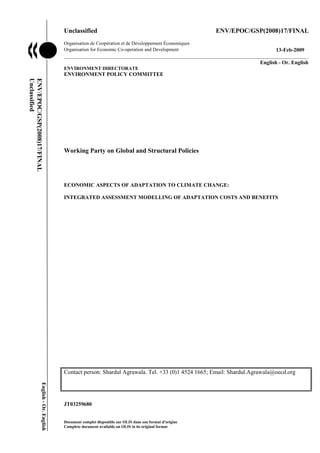
Using the parameter values for AD-DICE an adaptation cost curve can be drawn, as shown in
Figure 1. The figure shows that the adaptation costs of the first 15% of gross damage reduction are
extremely low after which they rise. In our calibrated model, the optimal level of adaptation varies from
0.13 to 0.34, with an average of 0.27, that is 27 percent of gross damages are reduced due to adaptation.
It can easily be seen that the costs of adaptation rise to such a high level that it can never be optimal to
fully adapt to climate change. In other words, solely adapting to climate change is not a solution and
mitigation will be needed too.
Figure 1. The adaptation cost curve implicit in the DICE2007 model (range 0.15-0.4).
3.2 RICE and AD-RICE
RICE is a regional version of the Dynamic Integrated Climate and Economy model. It consists
of 13 regions in the RICE99 online version. The regions are: Japan, USA, Europe5
, Other High Income
countries (OHI)6
, Highly Industrialised Oil exporting regions (HIO)7
, Middle Income countries (MI)8
,
Russia, Low-Middle income countries (LMI)9
, Eastern Europe (EE), Low Income countries (LI)10
,
5
Austria, Belgium, Denmark, Finland, France, Germany, Greece, Greenland, Iceland, Ireland, Italy, Liechtenstein,
Luxembourg, Netherlands, Norway, Portugal, Spain, Sweden, Switzerland, and the United Kingdom
6
Includes Australia, Canada, New Zealand, Singapore, Israel, and rich island states
7
Includes Bahrain, Brunei, Kuwait, Libya, Oman, Qatar, Saudi Arabia, and UAE.
8
Includes Argentina, Brazil, Korea, and Malaysia.
9
Includes Mexico, South Africa, Thailand, most Latin American states, and many Caribbean states.
10
Includes Egypt, Indonesia, Iraq, Pakistan and many Asian states.

15
China, India and Africa11
. The RICE model is a growth model. Each region has its own production
function which uses labour capital and energy inputs. The RICE model does not have an explicit
mitigation variable but mitigation is incorporated implicitly in specification of the carbon energy input.
The damage function of RICE is of the same form as that of DICE, however, in RICE some
regions can experience net benefits from climate change whereas in DICE the global average impact was
always negative. For example in colder regions, the warming of the climate can make previously
unutilized land arable (cf. IPCC, 2007b). Further detail on the mathematical formulation for of the net,
gross and residual damage functions and of the protection/adaptation costs is provided in Annex 3.
3.2.1 Calibration of AD-RICE
The online RICE99 model is used for this analysis. The model is calibrated in such a way that it
best replicates the results of the optimal control scenario of the original RICE model. Three regions (EE,
OHI and Russia) were excluded from the calibration as they have very low, near zero, net benefits from
climate change. Parameter values can be found for these regions but the information available is too
weak to obtain reliable estimates. The result of the calibration is provided in Annex 3.
The adaptation cost curves for the remaining 10 regions are drawn in Figure 2. The line
denominated as GLOBAL has been added and represents the AD-DICE 2007 global adaptation cost
curve (from Figure 1). For the three regions not calibrated (EE, OHI and Russia), it was assumed that no
adaptation will take place as the damages are so close to zero.
11
Includes all sub Saharan African countries, except Namibia and South Africa

16
Figure 2. Adaptation costs curves implicit in the RICE model.
0%
1%
2%
3%
4%
5%
6%
0.01
0.04
0.07
0.10
0.13
0.16
0.19
0.22
0.25
0.28
0.31
0.34
0.37
0.40
0.43
0.46
0.49
0.52
0.55
0.58
adaptation (fraction by which gross damages are reduced)
adaptationcostsasapercentageofoutput
JAPAN
USA
EUROPE
HIO
MI
LMI
LI
CHINA
INDIA
AFRICA
GLOBAL
As can be seen the adaptation costs in the different regions vary widely. Due to the limited
information with which these curves are estimated, these curves are only tentative, and may not fully
reflect the options available to individual regions. Clearly, such a top-down approach as the one
presented here will miss many relevant aspects of adaptation at the local level. Nonetheless, it is relevant
for examining the interaction between adaptation and mitigation at a macro level.
The relation between high estimated damages and high estimated adaptation costs for full
adaptation is straightforward: the higher the damage level, the more effort it will take to avoid all these
damages. As our variable for adaptation effort reflects an effort to avoid damages as a fraction, the
interpretation in absolute terms is different: where a single adaptation measure (say a flood protection
measure) may reduce 1 percent of all gross damages in one region, it may only reduce half a percent in
another region that has higher damage levels. Consequently, one can observe that the extremely high
adaptation costs for high adaptation levels are associated with regions that have high damage levels.
It should be stressed that the extremely high adaptation costs as projected by the curves for
several regions when adaptation efforts approach one, i.e. when almost all damages are avoided by
implementing adaptation measures, will never materialise. In this model the marginal adaptation costs
will always be balanced with the marginal avoided damages. Thus, it is not likely that the end of the
adaptation cost curve is reached: for the first adaptation measure the avoided damages are high and the
associated adaptation costs are low, but as more adaptation measures are implemented this ratio shifts. At
some stage, the additional cost of one more adaptation measure will not be outweighed by the avoided
damages, and it is no longer optimal to increase the adaptation effort.
4. Policy simulations with AD-DICE and AD-RICE
This section first compares the baseline scenarios of AD-DICE and AD-RICE with the IPCC
SRES scenarios. Next these models are used to run reference scenarios, to investigate the three cost

17
components of climate change (adaptation costs, mitigation costs, and residual damages) as well as the
interactions between adaptation and mitigation. Mitigation scenarios are then run to investigate the
effects of different proposed mitigation policies and what effects adaptation has on these policies. Finally
adaptation scenarios are run to understand the effects of under or over investment in adaptation.
4.1 Baseline Scenario Comparison
The baselines for AD-DICE and AD-RICE are compared with the common SRES storylines
developed by the IPCC. Comparisons are made along three projections: emissions, temperature change,
and output. Projections of emissions are made to verify that the models predict the same levels of
emissions in the baseline. Temperature change comparisons are used to verify that these emissions are
translated into temperature change in the same range in AD-DICE and AD-RICE as they are in the
SRES. Finally projections of output are compared to verify that the economic expectations given climate
change are in the same range. These comparisons are shown in Figures 3a-c.
Figure 3a. Emission estimates of the IPCC SRES and baseline scenarios of AD-DICE and AD-RICE
0.00
5.00
10.00
15.00
20.00
25.00
30.00
35.00
40.00
1990 2000 2010 2020 2030 2040 2050 2060 2070 2080 2090 2100
years
emissionsperyearinGtC
A1
A2
B1
B2
AD-DICE
AD-RICE
A1T

18
Figure 3b. Temperature estimates of the IPCC SRES and baseline scenarios of AD-DICE and AD-RICE.
0
0.5
1
1.5
2
2.5
3
3.5
4
4.5
5
1990 2000 2010 2020 2030 2040 2050 2060 2070 2080 2090 2100
years
temperaturechangefrom1900indegreesCelcius
A1
A2
A1T
B1
B2
AD-DICE
AD-RICE
Figure 3c. Output estimates of the IPCC SRES and baseline scenarios of AD-DICE and AD-RICE
0
100
200
300
400
500
600
1990 2000 2010 2020 2030 2040 2050 2060 2070 2080 2090 2100
years
outputintrillionsof$peryear
A1
A2
A1T
B1
B2
AD-DICE
AD-RICE
As shown in the above figures, the AD-DICE baseline generally falls within the SRES range
and seems to most closely correspond to the B scenarios. The AD-RICE model, however, is somewhat on

19
the low side for all indicators and falls beneath the SRES range. This is because the RICE model as used
to construct AD-RICE, unlike DICE, has not been updated. Nordhaus (2007) compares the DICE99
model to the updated DICE2007 model and identifies large differences in global output and other
variables. Furthermore damages were much lower in the older version.
Consequently, AD-DICE is the better model to investigate the interactions between adaptation
and mitigation on a global scale, and AD-RICE should only be used for those comparisons where a
regional differentiation is required. This principle (AD-DICE wherever possible, AD-RICE where
regional specificity is needed) is therefore used in the analysis of the scenarios in the sections below.
4.2 Reference Scenarios
Four reference scenarios are used here for AD-DICE and AD-RICE: no control, optimal
control, only adaptation and only mitigation; these are given in box 1. In the no control scenario,
adaptation and mitigation levels are set at zero.12
In “optimal"13
control, both adaptation and mitigation
levels are determined endogenously within the model to maximise discounted (present value) utility from
consumption, i.e. for both variables optimal levels are chosen. In the only adaptation scenario,
adaptation is at its optimal level while the mitigation level is zero. In the only mitigation scenario, the
mitigation is at its optimal level while the adaptation level is zero.
Box 1. Reference scenarios
R1. No Control: Neither mitigation nor adaptation is employed, i.e. no climate policies are applied.
R2. “Optimal”: Mitigation, adaptation, consumption are set at a level to maximize the value of net
economic consumption discounted over income per capita. Both the optimal mitigation and adaptation
policies are applied.
R3. No mitigation, optimal adaptation: Only adaptation can be used to combat climate change. The
optimal adaptation policy is applied.
R4. No Adaptation, optimal mitigation: Only mitigation can be used to combat climate change. The
optimal mitigation policy is applied.
The utility of the different scenarios is shown in Figure 4. A utility index is used, where the
level of utility in the optimal scenario is set at 100. The optimal control (R2) leads to the highest welfare
level. This is followed by the only adaptation scenario (R3) and the only mitigation scenario (R4), which
have similar levels of utility. Finally the scenario that creates the lowest utility is the no control scenario
(R1). These results confirm the importance of adaptation.
12
It should be noted that in AD-DICE mitigation will not be exactly zero, as the model contains some mitigation
efforts due to the exhaustion of fossil fuels (the Hotelling rents, which do not represent a policy option).
13
The term “optimal” throughout this report refers to outcomes from the optimisation framework of the DICE and
RICE models to maximise social welfare (utility) and are not intended to be policy prescriptive. Other models can
result in different optimal outcomes. Further, alternate assumptions with regard to discount rates and damage
functions within DICE and RICE can also change optimal outcomes. This is analysed in the sensitivity analysis in
Section 5.

20
Figure 4. Utility index for the policy scenarios
R1
R2
R3 R4
98.8
99
99.2
99.4
99.6
99.8
100
100.2
UtilityIndex
R1: No Controls
R2: Optimal control
R3: No Mitigation
R4:No Adaptation
While utility is the objective of the optimization procedure in DICE and RICE, it may be useful
to look at other indicators of economic prosperity as well. Therefore, the net present value (NPV) of
GDP per capita is given in Figure 5. As the level of GDP per capita is closely related to consumption
levels per capita (which are the determinant of utility), utility and the NPV of GDP per capita mostly
move in the same direction. Thus while the combination of both controls (the R2 optimal control
scenario) is superior to having only one control variable, only adapting (no mitigation scenario R3)
results in a lower GDP per capita than only mitigating (no adaptation scenario R4). In fact, when optimal
mitigation is still available, GDP levels are hardly affected by the availability of adaptation, as shown by
the negligible difference between R2 and R4.
However, when mitigation is unavailable, adaptation can prevent large GDP-losses, as shown
by the significant difference between R3 and R1.
There are clear differences between utility and the NPV of GDP per capita, especially for the
influence of adaptation. The main rationale for this is that the marginal utility of consumption per capita
decreases with increasing income (GDP) levels, and as GDP levels increase substantially over time, the
large future mitigation benefits have a larger impact on GDP per capita than on utility. For adaptation,
the benefits are more evenly spread over time.

21
Figure 5. NPV of GDP per capita for the policy scenarios
R1
R2
R3
R4
2.15
2.2
2.25
2.3
2.35
2.4
2.45
NPVofGDPperCapitainmillions$
R1: No Controls
R2: Optimal Controls
R3: No Mitigation
R4:No Adaptation
4.2.1 The Composition of Climate Change Costs
The costs of climate change include residual damages, adaptation costs and abatement (or
mitigation) costs. The composition of these costs is assessed over time at the global level using AD-
DICE for the reference scenarios. This is followed by an exploration of the regional differences using
AD-RICE.
Table 2 presents the components of climate costs in absolute terms (billion USD per year) for
four specific decades. In the very short run (2025-2034) the damages from climate change and the costs
of both adaptation and mitigation are relatively small. When no action is taken (R1), residual damages
amount to 204 billion USD globally each year in the decade 2025-2034. However, the total costs are
lowered only slightly (by 6 billion USD annually) by investing in both mitigation and adaptation
(compare R2 and R1) in this time horizon. Looking a bit further in time (2045-2054) the total costs can
now be reduced by 100 billion USD annually by investing in adaptation and mitigation (compare R2 and
R1). The required investments in this case amount to 56 billion dollars for mitigation and 27 billion USD
for adaptation annually, but decrease residual damages by 183 billion USD annually. In the scenario
without adaptation (i.e. mitigation only) the climate costs are substantially higher than in the scenario
without mitigation, even though residual damages do not differ much. Thus, in this case, adaptation only
(R3) can reduce 132 billion USD of annual residual damages at a cost of 31 billion USD, whereas
mitigation only can reduce 78 billion USD of residual damages at a cost of 85 billion USD. Thus, in the
short run adaptation is more effective at reducing residual damages than mitigation. However, this short-
term reasoning is flawed as it ignores the long-term benefits of mitigation.

22
Table 2. Build-up of climate costs in the reference scenarios in billion USD per year
Annual costs
(billion USD) R1 R2 R3 R4
Period 2025-2034
Adaptation costs 0 7 7 0
Mitigation costs 0 21 0 30
Residual damages 204 170 174 199
Total Costs 204 198 181 229
Period 2045-2054
Total Costs 695 595 594 703
Period 2095-2105
Total Costs 5430 3639 4281 4435
Period 2145-2155
Total Costs 22084 12311 16341 14936
At the beginning of the 22nd
century (2095-2105), the climate stakes are higher, as shown in
Table 2. In the case of inaction, residual damages would have risen to 5.4 trillion USD annually in the
decade, but nearly a half of those damages can be avoided by spending 247 and 367 billion USD
(annually) on adaptation and mitigation respectively. As time goes on mitigation becomes a more
important option (compare R3 and R4 over time), induced by the larger damages and longer lag time of
mitigation benefits. Note furthermore that the benefits of mitigation (in the form of reduced damages)
increase even more rapidly over time, as these reflect a combination of past and current mitigation
efforts. Clearly the uncertainties surrounding these projections for such long time periods are very high
and absolute numbers should be treated with caution. These projections, however, serve to highlight how
adaptation and mitigation affect total climate costs over time. Given the inertia in the climate system, the
benefits of mitigation policies become progressively more significant in later time periods. Therefore, a
long-term perspective is required to fully examine the relationships between adaptation and mitigation.
The composition of climate change costs in the optimal scenario meanwhile can be examined
over time by looking at Figure 6. As shown in this figure a large part of climate change costs under this

23
optimal scenario for all time periods consist of residual damages. In the optimal control scenario,
adaptation costs rise only slightly over time, while mitigation costs increase relatively steeply. As these
results are expressed in percentage of GDP, the increasing GDP levels imply that absolute expenditures
on adaptation are increasing substantially over time. It should be stressed that the optimal scenario
identified in the AD-DICE model does not imply a strict limit on CO2 concentrations: concentrations of
CO2 (excluding other greenhouse gases) peak around 680 ppm near the end of the 22nd
century, and the
associated temperature increase is almost 3.5°C. This is a much higher target of concentration and level
of climate change identified as “acceptable” in a number of other studies. Several reasons account for the
high DICE results, including a relatively high discount rate and low damage estimates compared to some
other IAMs. The sensitivity of the analysis to these assumptions is examined in detail in Section 5.
Furthermore, damages from extreme events and important irreversibilities are not included in the
analysis.
Figure 6. Composition of climate change costs in the optimal scenario
0.0%
0.5%
1.0%
1.5%
2.0%
2.5%
3.0%
3.5%
4.0%
4.5%
5.0%
2005
2025
2045
2065
2085
2105
2125
2145
2165
2185
years
costsaspercentageofoutput
Mitigation costs
Adaptation costs
Residual damages
Gross damages
While these graphs provide useful insights into the global components of climate costs, there
are substantial regional differences. These are depicted using AD-RICE for the optimal control scenario
in Table 3. In line with the existing insights from the literature (such as IPCC 2007b), the model
simulations here suggest that climate change will particularly affect many developing countries and
regions. Gross damages (in percentage of GDP) are projected to be especially high for India and Africa
(cf. Figure 2), and it is thus not surprising that the largest adaptation efforts are made in these regions.
Damages in Africa especially include health effects (75% of damages at 2.5 degrees of climate change).
Damages in India are caused predominantly in agriculture, health, and as a result of catastrophic events.
Residual damages are more evenly spread across regions, although clearly regions that have very small
gross damages will also have the lowest residual damages.14
At the other end of the spectrum, Nordhaus
and Boyer (2001) project in their RICE model that Japan will have small but positive net benefits from
14
As with most IAMs, the original RICE model, and consequently the AD-RICE model project fairly low damages
estimates for China, even though may have severe flood problems in the highly developed coastal areas. This is
again due to benefits in agricultural and increased amenity values, furthermore extreme weather events are not fully
considered in this model underestimating damages in regions with high damage potential from such events.

24
climate change for the coming century, due to their benefits for agriculture and increased amenity values
(see Annex 1 for detail on the RICE damage function). The AD-RICE model mimics these findings and
projects a small negative number for gross damages in Japan, and thus adaptation costs remain relatively
small. Note that the global numbers from these simulations with AD-RICE are not directly comparable to
the global AD-DICE results, as the level of damages is much lower in RICE – and thus in AD-RICE –
than in DICE – and thus AD-DICE.
Table 3. Regional components of damage and adaptation costs in the optimal control scenario, as projected
by the AD-RICE model, expressed as a percentage of regional GDP.
NPV Gross
damages
NPV
Residual
damages
NPV
Adaptation
costs NPV GDP
NPV Gross
damages as a
percentage of
NPV GDP
JAPAN -8 -91 25 183491 0.0%
USA 985 21 94 443078 0.2%
EUROPE 3852 2773 254 430159 0.9%
OHI 0 0 0 91864 0.0%
HIO 576 375 39 39442 1.5%
MI 2026 1497 133 183915 1.1%
RUSSIA 0 0 0 41081 0.0%
LMI 3440 2239 237 219515 1.6%
EE 0 0 0 55861 0.0%
LI 3237 2080 223 122537 2.6%
CHINA 277 33 39 166074 0.2%
INDIA 4661 2925 328 101871 4.6%
AFRICA 2051 1333 140 48598 4.2%
Global
(AD-RICE) 21097 13184 1515 2127485 1.0%
4.2.2 Adaptation-mitigation interactions
This section focuses on the interactions between adaptation and mitigation over time.
Furthermore the NPV of costs and benefits of each control in the various scenarios is examined.

25
Figure 7. Climate change costs (i.e. adaptation costs, mitigation costs and residual damages) over time for
the different policy scenarios
0%
1%
2%
3%
4%
5%
6%
2005
2015
2025
2035
2045
2055
2065
2075
2085
2095
2105
2115
2125
2135
2145
2155
years
climatechangecostsaspercentageofoutput
R1: No
Controls
R2:
Optimal
Controls
R3: No
Mitigation
R4: No
Adaptation
The distribution of costs of climate change over time with the different policy scenarios is
shown in Figure 7. As this figure shows, different scenarios distribute the costs of climate change quite
differently over time. Thus changes in the discount rate will also change the ranking of the scenarios. The
sensitivity of AD-DICE to assumptions about discount rates and damage functions is further examined in
Section 5. Figure 7 furthermore shows that the optimal scenario has the least discounted climate change
costs, while the no controls scenario has the highest discounted costs.
To examine the dynamics of adaptation and mitigation in more detail, the net benefits of
adaptation and mitigation over time (both as a percentage of output) are examined in Figure 8. The net
benefits of adaptation are calculated by comparing the residual damages in the scenarios with and
without adaptation, i.e. by comparing scenarios R2 and R4 when assuming optimal mitigation and R3
and R1 when assuming zero mitigation. Similarly, the net benefits of mitigation are calculated by
comparing scenarios R3 and R2 for optimal adaptation and R1 and R4 for no adaptation. The figure
shows that adaptation has higher benefits initially, while mitigation becomes much more beneficial than
adaptation over the long term. Thus even though it is optimal to start investing in mitigation
immediately, few of these benefits will be felt in the initial decades – largely because of the considerable
lags in the climate system.

26
Figure 8. Net benefits of adaptation and mitigation in different scenarios
-0.5%
0.0%
0.5%
1.0%
1.5%
2.0%
2.5%
3.0%
2005
2015
2025
2035
2045
2055
2065
2075
2085
2095
2105
2115
2125
2135
2145
2155
years
percentageofoutput
Benefits of
adaptation with
optimal
mitigation
Benefits of
adaptation with
zero mitigation
Benefits of
mitigation with
optimal
adaptation
Benefits of
mitigation with
zero adaptation
Figure 8 also illuminates the interactions between adaptation and mitigation. The net benefits of
mitigation are given for the case when only mitigation is an option and for the case where optimal
adaptation is also possible. It can be seen (by comparing the benefits of mitigation with and without
adaptation) that including adaptation as an option slightly increases the benefits of the optimal path of
mitigation until 2035 (although the effects are so small that this is not clearly visible from the figure) but
substantially decreases the benefits later. This is because adding adaptation as a control option will
decrease the optimal level of mitigation. Because of this some costs of mitigation in the beginning
periods will be avoided but this also entails that benefits of mitigation in later periods are lost. In other
words, when the option of adaptation is available one does not need to over-invest in mitigation in earlier
periods. Note that the analysis here does not consider direct interactions between adaptation and
mitigation. The possibility of such direct effects was surveyed in the IPPC’s 4th
Assessment Report
(IPCC 2007 Chapter 18) which concludes that the direct relationship between adaptation and mitigation
is ambiguous and likely to be small.
There is a chance that policymakers do not look at the optimal control over time but only
consider the near future. In other words, the world has a myopic view. In this case, because the benefits
of adaptation are higher in earlier years, there may be an overinvestment in adaptation and an
underinvestment in mitigation. This is a problem of intergenerational externalities: the burdens of
mitigation are felt in earlier periods, while the benefits are reaped in later periods (or more accurately the
benefits of a high level of consumption are reaped now, while the burdens are felt by later generations in
the form of climate change damages).
Figure 8 also shows that adaptation is less beneficial when mitigation is also an option. This is
because mitigation reduces gross damages reducing the potential benefits of adaptation. The difference
between benefits of adaptation with optimal mitigation and without mitigation increases over time,
because the effect of mitigation becomes more pronounced over time. It is important to note that even
though mitigation and adaptation decrease each other’s effectiveness, i.e. there is a negative interaction
effect, the simultaneous use of both options is still optimal. The marginal costs of both options increase
more than proportionately with higher percentages of mitigation/adaptation, and this effect is stronger
than the interaction effect, and the optimal policy involves a mixture of moderate amounts of both
adaptation and mitigation.

27
The framework can also be used to examine costs of inaction, i.e. if neither mitigation nor
adaptation is applied in the near future. For adaptation, the benefits occur immediately. Therefore the
absence of adaptation will lead to a loss of GDP, even in the short term. However, the absence of
mitigation may actually boost income levels initially. This reflects the delayed benefits of mitigation
actions, while the costs are near term. However, the absence of either or both mitigation and adaptation
will result in lower discounted utility relative to action on both mitigation and adaptation. Therefore
climate policies cannot be based on short-term insights and short-term net benefits only, i.e. a myopic
view could give the impression that postponing mitigation efforts is beneficial, but these short-term
benefits are more than outweighed by the long-term additional losses of inaction.
4.3 Mitigation scenarios
This section examines the effect of different mitigation policies, specifically policies which put
different caps on the level of temperature change or the amount of CO2 concentrations in the atmosphere.
Note that the DICE and RICE models only contain CO2, and the impact of other greenhouse gases only
enters the model through an exogenous additional radiative forcing parameter.
Box 2. Mitigation policy scenarios
M1 Concentrations are limited to 450 ppm.
M2 Concentrations are limited to 450 ppm after 2150. Overshooting is allowed.
M3 Concentrations are limited to 560 ppm (2x pre-industrial levels).
M4 Temperature increase is limited to 2 C from 1900 levels.
M5 Temperature increase is limited to 3 C from 1900 levels.
Figure 9 shows the composition and magnitude of the climate change costs for the mitigation as
well as the reference scenarios. The figure shows firstly that residual damages can be decreased severely
by mitigation and adaptation. This can be seen by comparing R1 with the other scenarios. Secondly, as
mitigation policies become more stringent adaptation decreases, in M1 adaptation costs are virtually
zero. Thirdly, the absence of adaptation boosts mitigation efforts, but only moderately (compare R2 and
R4). Not surprisingly, the stringency of the climate policy target is more important for mitigation efforts
than the availability of adaptation as a policy option. Fourthly, note that the climate change costs are
lower in the mitigation scenarios M1-M5 than in the optimal (R2), whereas the utility is (by definition)
the highest in the optimal. This is due to that fact that utility reflects a discounting of costs over time (to
reflect social time preference) and a decreasing marginal utility of consumption as income (and thus
consumption) levels rise over time. Compared to R2, scenarios M1-M5 require more investment in
mitigation in earlier decades, which results in lower residual damages in the later decades. This decreases
the total climate costs in present value terms, but also lowers the utility as the additional costs are borne
by earlier (poorer) generations whereas the lower residual damages are experienced by later (richer)
generations.

28
Figure 9. Composition of climate change costs
0
200
400
600
800
1000
1200
1400
R 1 R 2 R 3 R 4 M1 M2 M3 M4 M5
NPVintrillion$
adaptation costs
mitigation costs
residual damages
The mitigation scenarios (M1-M5, see Box 2) are examined in more detail in Table 4 where the
benefits/costs of mitigation are computed with (optimal) adaptation, as well as without adaptation. The
benefits of the mitigation policies generally decrease when adaptation is possible. What is more
interesting is that the benefits/cost ratio does not increase evenly across scenarios when adaptation is not
available. This shows that the effectiveness of different mitigation scenarios is somewhat dependent on
the use of adaptation. The ranking of the scenarios does not change in this case. Thus it can be tentatively
concluded that adaptation does not significantly change the results on the preference of a certain
mitigation scenario compared to other mitigation scenarios. However, though the general conclusions
based on optimal adaptation are valid, they may not properly describe all relevant variables involved,
such as the magnitude of benefits from mitigation.
Table 4. The costs and benefits of mitigation in different scenarios
NPV of
benefits
NPV of
costs
Benefit/ NPV of
benefits
NPV of
costs
Benefit/
cost ratio cost ratio
Mitigation with adaptation Mitigation without adaptation
M1
859.44 249.81 3.44 1240.59 237.31 5.23
M2
835.14 215.04 3.88 1210.42 202.00 5.99
M3
674.41 113.96 5.92 1023.13 105.84 9.67
M4
797.03 181.70 4.39 1164.54 169.26 6.88
M5
643.16 102.87 6.25 983.37 94.59 10.40
4.4 Adaptation scenarios
This section examines the effects of different restrictions on adaptation. There are many
reasons why the optimal level of adaptation may not be attainable (see for example, IPCC2007b, Chapter
17). This section discusses some of the key constraints and limits to adaptation, and “adaptation
scenarios” are then constructed to look at the effects hereof (Box 3).

29
An often mentioned limitation to adaptation is that of lack of knowledge. The exact effects of
climate change may not be known or the adaptation measures to be taken may not be known to the
people concerned (Fankhauser, 1997). These limitations are mimicked, albeit in a crude fashion, in
scenarios A1 and A2, where the amount of adaptation is limited.
A second issue is the problem of not having enough funds to adapt. For example a farmer may
not have enough money to invest in seeds for new crop types or a government may not have the funds to
build a sea wall. This limitation is usually mentioned with reference to developing countries (scenario
A3), but there is a qualification (c.f. MacMichaels, 1996, and Fankhauser, 1998) that it concerns the
poorest individuals in each country (scenarios A4 and A5).
A third constraint on adaptation entails inertia (cf. Burton and Lim 2005): adaptation levels
may not be able to change (quickly) over time (scenario A6). A different type of inertia refers to the
problem of a delayed reaction (scenario A7). It might take considerable time to implement adaptation
measures (Mendelsohn, 2000, and Berkhout et al., 2006). Finally it may be the case that because of
imperfect knowledge there are over-investments in adaptation. This is simulated in A8 and A9.
Box 3. Adaptation policy scenarios
Limits on adaptation
A1 Adaptation can only be 50% of optimal
A2 Adaptation can only be 75% of optimal
Limits on adaptation costs
A4 Adaptation costs can only be 50% of optimal
A5 Adaptation costs can only be 75% of optimal
Rigidness of adaptation
A6 The level of adaptation cannot vary over time
A7 Adaptation cannot be implemented in the first 30 years
Overinvestment in adaptation
A8 Adaptation is set at a level 125% of the optimal
A9 Adaptation is set at a level 150% of the optimal
Note: Mitigation is set at optimal levels in all these scenarios
Figure 10 shows how the different adaptation scenarios affect utility. To ease comparison
utility differences compared to the optimal control scenario (R2) are used. For reference purposes the no-
adaptation scenario (R4) is also shown. Not surprisingly, the more stringent restrictions on adaptation
affect utility more than those scenarios that are closer to the optimum.
The results also show that limits on the funds available for adaptation are less harmful than
limits on adaptation efforts themselves. But bearing in mind that the A1 and A9 scenarios are rather
extreme, the overall conclusion can be that as long as mitigation options can be freely chosen, most
limitations on adaptation will have only very minor influence on global welfare. This does not mean that

30
some regions will not incur severe losses when adaptation is limited. Thus, uncertainty about the exact
optimal amount of adaptation should not prevent investment in adaptation, but caution is warranted:
choosing the adaptation level should be done with care and more adaptation is not always better. Still, it
is preferable to over-invest or under-invest than to not invest at all (R4).
Figure 10. Utility difference compared to optimal of different adaptation scenarios in the AD-DICE model.
A5
A4
A2 A7
A6 A8
A1
A9
R 4-0.30%
-0.25%
-0.20%
-0.15%
-0.10%
-0.05%
0.00%
Percentagedifferenceinutiltiycomparedto
optimal
A5
A4
A2
A7
A6
A8
A1
A9
R 4
5. Sensitivity analysis
This section assesses the sensitivity of the models used here and the results presented. It first
looks at the effects of applying different discount rates in DICE and then at how a higher damage
function will affect the results.
5.1 Alternative Discounting
One of the major points of discussion within cost-benefit analysis of climate change is that of
the discount rate. Often the DICE model formulation by Nordhaus is criticized for having a too high
discount rate. To test the effect of the discount rate assumptions we run several key scenarios from our
analysis using different discount rate specifications. We have chosen to use two discount rates, suggested
respectively by the UK Treasury and that applied in the Stern Review.
The discount rates are determined based on the Ramsey equation. This equation states that the
discount rate is equal to ρ + µg, where ρ is the rate of pure time preference, µ represents the absolute
value of the elasticity of marginal utility, and g the per capita growth rate of consumption. The first term
ρ in the Ramsey equation reflects the discount rate that would apply if future generations had the same
wealth as the current generation. The second term µg is the wealth-based component and reflects the
assumption that one extra dollar is worth more to a person with a low income than to a person with a
high income. The different assumptions on these parameters for the different discounting methods are
given in Table 5. Note that because DICE endogenously estimates economic growth, the assumptions
about that are not changed within the model.

31
Table 5. The parameter values assumed in the different discounting methods
Method µ = elasticity of marginal
utility of consumption
ρ =pure rate of time
preference
Nordhaus 2 1.5
UK Treasury 1 1.5
Stern 1 0.1
In Figure 11 the different discount rates are plotted over time. Due to the fact that we use
endogenous economic growth the discount rates have similar forms but vary in magnitude. As can be
seen, the DICE discount rate chosen by Nordhaus is the highest, the Stern Review the lowest and the UK
Treasury lies in between.
Figure 11. Discount rates over time for the different discounting methods.
0
0.5
1
1.5
2
2.5
3
3.5
4
4.5
5
2005
2015
2025
2035
2045
2055
2065
2075
2085
2095
2105
2115
2125
2135
2145
2155
2165
2175
2185
2195
years
Discountratein%
UK treasury
Stern
Nordhaus

32
Figure 12. CO2 concentration levels (in ppm) over time for the different discounting methods
350
400
450
500
550
600
650
700
750
2005
2015
2025
2035
2045
2055
2065
2075
2085
2095
2105
2115
2125
2135
2145
2155
2165
2175
2185
2195
years
ConcentrationsofCo2inatmosphere(inppm)
Nordhaus
R2:Optimal Controls
UK treasury
R2:Optimal Controls
Stern
The concentration levels of CO2 in the optimal scenarios using the different discounting
methods are given in Figure 12. There are large differences between the optimal levels of concentrations
with the different discounting methods. According to the Stern Review, the optimal level of
concentration peaks at a level slightly above 400 ppm whereas the Nordhaus optimal level of
concentrations is above 650 ppm. The Treasury’s discount rate suggests an optimal level peaking at 550
ppm. It can be seen that the high discount rate used by Nordhaus causes the optimal level of CO2 to be
significantly higher than when using alternative discounting methods.
To investigate if the discounting method has effects on the different scenarios, the reference
scenarios are re-run using the Stern Review and UK Treasury discounting methods (R1: no controls, R2:
optimal, R3: no mitigation, R4: no adaptation). In Figure 13 the relative utilities of the scenarios are
shown for each discounting method. Due to the higher discount rate applied, and therefore a more short-
sighted view, adaptation plays a more important role as a policy option in the Nordhaus discounting
scenarios (the R4 utility is lower than R3) than in the other two settings. The Stern Review discounting
puts much more weight on future generations causing a higher level of mitigation to be optimal. This is
turns makes adaptation less beneficial. As can be seen in the figure adding the option of adaptation
makes very little difference to utility (compare R2 and R4). Using the UK Treasury discounting,
adaptation remains an important option but less important as mitigation.

33
Figure 13. Utility index for the reference scenarios using different discount rates
Nordhaus
R1
R4 R3
R2
98.8
99
99.2
99.4
99.6
99.8
100
100.2
UtilityIndex
UK Treasury
R1
R4
R3
R2
99.97
99.98
99.99
100
100.01
UtilityIndex
Stern Review
R1
R4
R3
R2
98.8
99
99.2
99.4
99.6
99.8
100
100.2
UtilityIndex
R1: No Controls
R4:No Adaptation
R3:No Mitigation
This is also reflected in the differences in the composition of climate change costs with the
different discounting methods. In Figure 14 the composition of climate change costs for each discounting
method is given. The Nordhaus discounting method has the highest residual damages and the lowest
mitigation costs. The Stern discounting leads to very low adaptation costs in this case.

34
Figure 14. Climate change costs compostion for different discount rates (percentage of total NPV of climate
change costs)
0%
10%
20%
30%
40%
50%
60%
70%
80%
90%
100%
Nordhaus UK treasury Stern
percentageoftotalclimatechangecosts
mitigation costs
adaptation costs
residual damages
To get a better understanding of the influence of the discounting method on the climate change
cost we present the different undiscounted climate change costs in Table 6. It can be sees that the amount
spent on adaptation is tenfold higher with the Nordhaus discounting than with the Stern Review
discounting. Thus this sensitivity analysis suggests that, as expected, a lower discount rate increases the
optimal level of mitigation and thus decreases the optimal level of climate change. As the DICE model
on which our main analysis is based uses a relatively high default discount rate, we should be careful in
interpreting the optimal policies that it suggests.
Table 6. Undiscounted climate change costs in AD-DICE between 2005 and 2105 in trillions of dollars.
Discounting method Adaptation Costs Mitigation Costs Residual Damages
DICE 10.5 16.5 139.3
UK Treasury 9.9 48.1 137.4
Stern Review 4.3 342.4 79.6
5.2 Alternative damage function
As mentioned earlier one critique of the DICE and RICE models is that the damage function is
low (although it must be noted that many other IAMs also use the DICE/RICE damage functions). This
section examines the effects of using a damage function that has higher damages. Recent estimates by
Michael Hanemann (2008a, b) suggest that damages could be 2.5 times higher than the DICE 2007
model suggests. Some key scenarios discussed earlier are re-run with a damage function that is scaled up
2.5 times.
Figure 15 shows the optimal levels of mitigation and adaptation using the original and the
scaled-up damage function in DICE. As can be seen both the adaptation and mitigation levels increase
when the damage function is scaled up. Furthermore the level of mitigation increases much more than
that of adaptation.

35
Figure 15. Optimal mitigation and adaptation levels (in percentages) with the original and scaled-up damage
functions
0
0.1
0.2
0.3
0.4
0.5
0.6
0.7
0.8
0.9
12005
2025
2045
2065
2085
2105
2125
2145
2165
2185
years
adaptationandmitigationlevel
mitigation (higher damage
function)
adaptation (higher damage
function)
mitigation (original)
adaptation (original)
As shown in Table 7, optimal peak levels in CO2 concentration are also much lower with the
higher damage function, which is intuitive.
Table 7. CO2 concentration (ppm) with different damage functions
Model 2055 2105 2155
AD-DICE (original) 492 596 672
AD-DICE (higher damages) 474 536 525

36
Figure 16. Utility of reference scenarios (AD-DICE) under a scaled up damage function
96
96.5
97
97.5
98
98.5
99
99.5
100
100.5
Utilityindex(R2=100)
R 1:no controls
R 3: no mitigation
R 4: no adaptation
R 2: optimal controls
An interesting issue is to look at the effect of a higher damage function on adaptation and
mitigation effectiveness. As can be seen in Figure 16, when damages are scaled up the scenario without
adaptation is no longer worse than that of no mitigation as with the original damage function. Thus a
higher damage function will increase the effectiveness of mitigation relative to adaptation. Once again it
can be concluded that the results given by the DICE model are likely to overestimate the role of
adaptation and the optimal level of climate change.
A scenario with higher damages has also been run using AD-RICE. As in the AD-DICE
sensitivity analysis, we choose for a value that is 2.5 times higher than in the base AD-DICE
specification; as the damage level in AD-RICE is about 40 percent lower than in AD-DICE, we multiply
the base AD-RICE values fourfold to get comparable damage levels15
. Table 8 shows that in net present
value terms, gross damages only increase 2.6 times. Thus, the higher damage function invokes more
substantial mitigation efforts to avoid these large damages. Implementation of adaptation measures
further reduces these damages: residual damages are just 2.4 times as high as in the base specification.
Note that these damage reductions do not come for free: the net present value of adaptation costs more
than triples. Most regional results follow the global trend.
15
For some regions, parameter α1 is negative, i.e. for small levels of temperature increase there are initial climate
benefits. To avoid that these benefits also get larger, only parameter α2 is rescaled such that gross damages are 4
times higher for a temperature increase of 2.5 degrees (more or less corresponding to a doubling of CO2
concentrations).

37
Table 8. Regional components of damage and adaptation costs in the Optimal control scenario in trillion
USD for the base model and increased damages (AD-RICE)
NPV gross damages NPV residual damages NPV adaptation costs
Base model
Higher
damages Base model
Higher
damages Base model
Higher
damages
JAPAN -1 31 -9 16 3 5
USA 99 163 2 26 9 13
EUROPE 385 996 277 647 25 82
OHI 0 0 0 0 0 0
HIO 58 166 37 92 4 14
MI 203 600 150 380 13 55
RUSSIA 0 0 0 0 0 0
LMI 344 902 224 511 24 77
EE 0 0 0 0 0 0
LI 324 870 208 479 22 75
CHINA 28 45 3 16 4 5
INDIA 466 1143 293 619 33 99
AFRICA 205 581 133 317 14 51
Global 2110 5495 1318 3103 151 478
Note: The climate costs projections reported here are based on relatively old estimates of damages in the RICE99 model, as
discussed in Annex 1, and may not reflect the latest scientific insights into the impacts of climate change on specific regions.
6. Concluding remarks
This report seeks to inform critical questions with regard to policy mixes of investments in
adaptation and mitigation, and how they might vary over time. This is accomplished here by examining
adaptation within global Integrated Assessment Modelling (IAM) frameworks that have explicit
treatment of the costs of mitigation, the costs of adaptation, and the residual damages from climate
change.
None of the existing IAMs captures adaptation satisfactorily. Many models do not specify the
damages from climate change, and those that do mostly assume implicitly that adaptation is set at an
“optimal” level that minimizes the sum total of the costs of adaptation and the residual climate damages
that might occur.
This report develops and applies a framework to include adaptation explicitly as a policy
variable in IAMs. By including adaptation into IAMs, these already powerful tools for policy analysis are
further improved, and the interactions between mitigation and adaptation can be analysed in more detail.
Specifically the approach is applied to two IAMs – the global Dynamic Integrated model for Climate and
the Economy (DICE) and its regional counterpart, the Regional Integrated model for Climate and the
Economy (RICE). These modified models – AD-DICE and AD-RICE – are calibrated and then used in a
number of policy simulations to examine the distribution of adaptation costs and the interactions between
adaptation and mitigation.
Based on this methodology, and keeping in mind the limitations of the model simulations, a
number of conclusions can be drawn. First, both mitigation and adaptation are important in responding to
climate change. A good adaptation policy matters; especially when suboptimal mitigation policies are
implemented. Similarly, a good mitigation strategy is more important when optimal adaptation levels are
unattainable. The rationale for this result is that both policy control options can compensate to some
extent for deviations from the efficient outcome caused by non-optimality of the other control option.
The policy simulations presented in this report suggest that overinvestment in adaptation may be worse
from a welfare perspective than underinvestment, although moderate overinvestment is still far

38
preferable to no adaptation at all. Thus, uncertainty about the exact optimal amount of adaptation should
not prevent investment in adaptation, but caution is warranted: choosing the adaptation level should be
done with care and more adaptation need not always be better.
Second, the higher the current value of damages the less important adaptation is as a policy
option in comparison to mitigation. The comparison between adaptation and mitigation therefore
depends crucially on the assumptions in the model, and especially on the discount rate and the level of
future damages. A lower discount rate changes the optimal mixture of policies away from adaptation
towards more mitigation and may thus imply lower adaptation efforts; for higher damage levels,
adaptation efforts increase, but the optimal level of mitigation will also increase, which dampens the
higher need for adaptation. The models used in this report adopt assumptions that imply that the current
value of damages is relatively low and in this case adaptation matters as much as mitigation. In all cases,
however, a good policy decision on the level of adaptation is an essential part of an optimal strategy to
combat climate change. The marginal costs of both adaptation and mitigation increase more than
proportionately with higher levels of the policy, and the optimal policy involves a mixture of both
adaptation and mitigation. As adaptation and mitigation both limit climate change damages, when one or
the other is set too low the other may compensate to some extent by taking a higher level.
Third, optimal adaptation efforts start at a reasonably high level immediately, whereas optimal
mitigation levels are slowly increasing over time. This is mainly related to the considerable lags in the
climate system: the benefits of adaptation are felt immediately, whereas the emission reductions achieved
through mitigation will lead to a stream of benefits in the future. Thus to combat climate change in an
efficient way, the short term optimal policy consists of a mixture of adaptation measures and investments
in mitigation, even though the latter will only decrease damages in later periods. The costs of inaction are
high, and thus it is more important to start acting even when there is a lack of information on which to
base the policies, than to ignore the problems climate change already poses. At the end of the 21st
century, the climate stakes have become substantial: the policy simulations presented here suggest that in
the case of prolonged inaction, damages may have risen to more than 5 trillion dollars annually, but a
third of those damages can be avoided by spending some 250 and 370 billion dollars annually on
adaptation and mitigation, respectively. The longer-term also consists of a mixture of adaptation and
mitigation policies, and ongoing increases in expected damages over time imply that adaptation is not an
option that should be considered only for the coming decades, but it is important to keep investing in
adaptation options, as both the challenges and benefits of adaptation increase.
Finally, at the regional level there are substantial differences in the optimal adaptation efforts:
especially in vulnerable regions, adaptation is an essential ingredient in the policy mix. Limitations to
adaptation may not have a substantial impact at the global level, but may induce severe climate damages
in vulnerable regions. Unfortunately, these are also the regions where funds and good information are
scarce, and thus it is especially hard to formulate good policies for these regions. The results presented in
this report suggest that in some less vulnerable regions adaptation may completely remove all damages,
and in principle even transform (gross) climate damages into (residual) climate benefits. Such
transformations are not available for free, however; the region will have to invest in adaptation to create
such opportunities. Note finally that while optimal adaptation unambiguously increases welfare in the
adapting region itself, it reduces the optimal level of mitigation for a given region, and therefore lowers
the positive spillovers of mitigation to other regions.
The above results, however, are subject to a number of caveats in the analysis and should
therefore be interpreted with sufficient care. Specifically, there are four major limitations. First, a main
caveat is the absence of detailed regional knowledge on damages and adaptation options to reduce these
damages. Thus, this analysis was confined to a top-down assessment, and the results could not be refined
with more detailed bottom-up information. A second caveat is the exclusion of uncertainty and risk. In
reality, policy decisions have to be made without full information, and the recent climate change
literature on low-chance, high-damage possibilities and hedging strategies stresses the weakness of

39
“point estimates” and deterministic analysis. A more systematic uncertainty analysis was beyond the
scope of the present work but should be a high priority for further research in this area. Third, the
formulation of adaptation in the model is a flow approach, i.e. adaptation is essentially seen as reactive.
A more elaborate stock-and-flow approach may be able to reflect the anticipatory nature of certain types
of adaptation measures better. Finally, it is important to stress that two specific existing models, DICE
and RICE, form the basis for this quantitative analysis. Optimal mitigation scenarios in these two models
do not imply stabilization of greenhouse gas concentrations at low levels; consequently, the results,
especially with respect to the optimality of slowly increasing mitigation levels, may be different when
other IAMs are used as the basis for analysis and it would be best if a canopy of models is used to
investigate the interactions between adaptation and mitigation to be able to derive robust policies. In the
sensitivity analysis presented in this report it is shown that running the models with a higher discount rate
or including a higher damage function leads to much higher levels of optimal mitigation.
This report opens the door for such alternative simulations as the methodology used can be
applied to other IAMs. Another extension of this work relates to the formulation of a combined “stock
and flow” approach to modelling adaptation where both near-term and lagged benefits of adaptation
actions are incorporated with IAMs.

40
REFERENCES
Agrawala, S. and S. Fankhauser (2008), “Putting climate change adaptation in an economic context” in
Economic Aspects of Adaptation to Climate Change: Costs, Benefits and Policy Instruments,
OECD, Paris.
Berkhout, F., J. Hertin and D.M. Gann, 2006: Learning to adapt: organisational adaptation to climate
change impacts. Climatic Change, 78, 135-156
De Bruin K, R. Dellink, and R. Tol (2008), AD-DICE: an implementation of adaptation in the DICE
model. Climatic Change, forthcoming.
Burton, I. and Lim, B.: 2005, ‘Achieving adequate adaptation in agriculture’, Clim. Change 70, 191–200.
Fankhauser, S. (1994), Protection vs. Retreat – The Economic Costs of Sea Level Rise. Environment and
Planning A, 27, 299-319.
Fankhauser, S. (1998), The costs of adapting to Climate Change. GEF Working Paper Series 16, Global
Environmental Facility.
Hanemann, M. (2008a). “Observations on the Economics of Adaptation: Uncertainty and Timing”. Paper
presented at the OECD Expert Workshop on the Economic Aspects of Adaptation to Climate
Change, April 7-8, Paris.
Hanemann, M. (2008b). What is the Economic Cost of Climate Change ? CUDARE working paper 1071,
University of California, Berkeley.
Hof AF, den Elzen MGJ, van Vuuren DP (2008). Analyzing the costs and benefits of climate policy:
Value judgements and scientific uncertainties. Global Environmental Change 18(3), 412-424.
Hope, C.W., J. Anderson, and P. Wenman (1993), Policy analysis of the greenhouse effect-an application
of the page model. Energy Policy, 15, 328-338.
Hope, C.W. (2006), The marginal impact of CO2 from PAGE2002: an integrated assessment model
incorporating the ipcc’s five reasons for concern. The Integrated Assessment Journal, 6 (1), 19-56.
Ingham A., J. Ma and A.M. Ulph (2005). How do the costs of adaptation affect optimal mitigation when
there is uncertainty, irreversibility and learning?. Tyndall Centre working paper 79.
IPCC, (2007), Fourth Assessment Report: http://www.ipcc.ch/activity/ar.htm#ar4.
Kelly, D.L. and C.D. Kolstad (1999), Integrated Assessment for climate control. In: H. Folmer and T.
Tietenberg (eds), International Yearbook of Environmental and Resource Economics 1999/2000:
A Survey of Current Issues, Edward Elgar, Cheltenham, UK.
Klein, R. et al. (2007) Adaptation to Climate Change in the Context of Sustainable Development and
Equity, IPCC (2007b), op.cit..
Lecocq, F. and Shalizi, Z. 2007. "Balancing expenditures on mitigation of and adaptation to climate
change : an exploration of Issues relevant to developing countries," Policy Research Working
Paper Series 4299, The World Bank.

41
McKibbin, W.J. and P.J. Wilcoxen (2004). Climate Policy and Uncertainty: The Role of Adaptation
versus Mitigation. Paper prepared for the Australian National Academies conference on “Living
With Climate Change”. http://www.msgpl.com.au/download/aas4.pdf
McMichael, A.J. (1997). Integrated Assessment of potential health impact of global environmental
change: prospects and limitations, Environmental modelling and assessment 2, 129-137.
Mendelsohn, R, Morrison, W, Schlesinger, M. E., Andronova, N. G. (2000). Country Specific market
Impacts of Climate Change. Climatic Change 45: 553–569, 2000.
Mendelsohn, R. (2000), Efficient adaptation to climate change. Climatic Change, 45, 583-600.
Nordhaus, W.D. (1994). Managing the Global Commons: The Economics of the Greenhouse Effect. MIT
Press, Cambridge, MA.
Nordhaus, W.D. and Z. Yang (1996), A Regional Dynamic General-Equilibrium Model of Alternative
Climate-Change Strategies, American Economic Review, 86(4), 741-765.
Nordhaus, W.D., and Boyer, J (2000) Warming the World: Economic Models of Global Warming. MIT
Press, Cambridge, ma.
Nordhaus, W.D. (2007), http://nordhaus.econ.yale.edu/dice_mss_091107_public.pdf.
OECD (2008) Economic Aspects of Adaptation to Climate Change, 133pp., OECD Paris
Parry, M., N. Arnell, M. Hulme, R. Nicholls, and M. Livermore, 1998: Adapting to the inevitable.
Nature, 395, 741-742.
Reilly, J., N. Hohmann, and S. Kane, 1994: Climate change and agricultural trade: who benefits, who
loses? Global Environmental Change, 4(1), 24-36.
Tol, R.S.J. and S. Fankhauser (1998), On the Representation of Impact in Integrated Assessment Models
of Climate Change. Environmental Modelling and Assessment, 3, 63-74.
Tol, R.S. J., Fankhauser, S. and Smith, J.B. (1998), The Scope for adaptation to climate change: what can
we learn from the impact literature? Global Environmental Change, 8(2), 109-123.
Tol, R.S.J., S. Fankhauser, R.G. Richels and J.B.Smith (2000), How Much Damage Will Climate Change
Do? Recent Estimates, World Economics,1(4), 179-206.
Tol, R.S.J. (2002), Estimates of the Damage Costs of Climate Change. Environmental and Resource
Economics, 21, 47-73.
Tol, R.S.J., (2005), Adaptation and Mitigation: Trade-Offs in Substance and Methods. Environmental
Science and Policy, 8 (6), 572-578.
Tol, R.S.J., (2008) The Double Trade-Off between Adaptation and Mitigation for Sea Level Rise: An
Application of fund. Mitigation and Adaptation Strategies for Global Change, forthcoming.

42
ANNEX 1.
UNRAVELING THE DAMAGE FUNCTION OF THE DICE AND RICE MODELS
Assessing the damages associated with climate change is a complicated and difficult issue due
to the wide range of climate change impacts and the large uncertainties involved. However, to formulate
optimal policies regarding adaptation and mitigation these damages need to be assessed and monetised.
Although the many different forms of damages make aggregation difficult, there have been several
attempts to create aggregated damage functions for major world regions. The most notable of these
attempts are those of Nordhaus in the DICE/RICE model (e.g. Nordhaus and Boyer 2001), Tol in the
FUND model (e.g. Tol 2002), Hope in the PAGE model (Hope et al. 2006) and Mendelsohn (e.g.
Mendelsohn et al., 2000).
To assess climate change damages in a comprehensive manner, damages are often divided into
different categories. The estimation of damages carries with it great uncertainties and is often based on a
mixture of extrapolating limited data, calibrating to existing information from the literature, applying the
expert “guesstimates” of the authors and ignoring impacts that cannot be assessed or monetised. The
damage function of DICE/RICE and its estimation and calibration are explained in detail in Nordhaus
and Boyer (2001). Their approach is briefly summarised here. As this is the damage function used in this
analysis, the results presented in this paper rely crucially on these damage estimates.
The Nordhaus damage function has seven damage categories: Agriculture, Other Vulnerable
Markets, Coastal, Health, Non Market Time Use, Catastrophic, and Settlements. Nordhaus’ regional
damages/benefits estimates for these seven categories are provided in Table 9.
The ‘Agriculture’ category refers to the damages in the agricultural sector due to climate
change. The damage estimates are based on studies done on crop yield variation under different
temperatures and precipitation using the FARM model. Assuming that crop production will be adjusted
to the new climate, the damages are assessed.
The ‘Other vulnerable markets’ category refers to the effect of climate change on other
markets. Nordhaus and Boyer conclude that the only significantly affected markets are energy and water.
More energy will be needed in some regions for air conditioning whereas colder regions will need less
energy for heating. Water use is also expected to increase, for example, due to increased irrigation needs.
Nordhaus and Boyer estimate these damages based on US data which are then extrapolated using the
average temperature effects in the other regions.
The ‘Coastal’ category refers to the damages due to sea level rise. As the climate warms, the
level of the sea rises. Adaptation options considered consist of either building sea walls to protect against
sea level rise (incurring protection costs) or accepting the land loss (incurring residual damages).
Nordhaus and Boyer use US estimates and extrapolate them based on a coastal vulnerability index (the
coastal area to total land area ratio).
The ‘Health’ category refers to all damages incurred due to malaria, dengue, tropical diseases
and pollution. Although heat- and cold-related deaths are also affected by climate change, they are not
included here. In general, regions that are already vulnerable to such diseases have large damages, and
thus developing regions tend to have the largest damages in this category.

ENV-EPOC-GSP(2008)17-FINAL

Recommended

Recommended

More Related Content

Viewers also liked

Viewers also liked (13)

Similar to ENV-EPOC-GSP(2008)17-FINAL

Similar to ENV-EPOC-GSP(2008)17-FINAL (20)

ENV-EPOC-GSP(2008)17-FINAL