ECTE901_AssignmentReport_v1.2

ECTE901 – A Web Graphic Format Introduction – Emeric Vigier – 26/05/2006 1/21
University of Wollongong
School of Electrical, Computer and Telecommunications Engineering
ECTE901 – Fast Signal Processing Algorithms
An Introduction on Web Graphic Formats
Emeric Vigier – ID: 2974526 – ev009@uow.edu.au
Friday, 26th
May 2006
Abstract – This study aims to introduce some
graphic formats widely used on the web today.
Through the history, the theory background and
some implementation examples, the JPEG and
PNG formats are here discussed. Some
transforms and codings are here described: DCT,
entropy coding, LZ77, Huffman coding and
Adam7 algorithm.
Keywords – Transform-based image coding,
JPEG, PNG, graphic format, compression, Cosine
Transform, entropy coding.
INTRODUCTION
Image compression is a wide field with many
applications, needs and features. The choice of a
compression format has to be made regarding
constraints such as file size, detail level, and
losing information acceptance. It is obvious that
storing an image of a pet on an online server and
saving an image of a FBI fingerprint in a
hundreds of million capacity database does not
require the same specifications (the reader
interested in very efficient technology, Discrete
Wavelet Quantization, that has been used by the
FBI can have a look at [5]). The World Wide Web
has been a convenient platform to evaluate
graphic formats along their apparition and
standard acceptation. Nowadays, there is a wide
distribution of graphic standards. Some of them
are patent-free, platform dependent or designed
for a specific use (satellite images, technical
drawings). Here, the purpose is to describe two
main and popular image formats. Websites and
web applications are using them depending on
many aspects such as cross-platform capability,
compression effectiveness, backward
compatibility or the Webmaster awareness. New
standards, such as JPEG-2000, or more effective
transforms, such as the wavelet transform, will
not be considered here because they have not
penetrated the web yet. For web applications, a
graphic format should have high compression
capability because the aim is often to show the
image clearly to human eyes but without keeping
useless details. It should also provide an efficient
interlacing capability to preview the picture while
downloading it.
1 Literature Review
Image compression has been a challenge of
high importance in telecommunications.
Researches on the topic points back to the 60’s
and have been improved in the 90’s with a lot of
related papers and graphic format releases.
1.1 History of Transforms
The history of the transforms used in Image
Processing starts with the Discrete Fourier
Transform. James Cooley, IBM T.J. Watson
Research Center, and John Tukey, Princeton
University, succeeded to execute the Fourier
Transform on a computer in 1965. Their
following publication made it possible to control

the power of Fourier analysis in computational
work [2].
The NASA implemented an adaptation of this
transform, called Discrete Cosine Transform, in
the early 1960’s for processing images. This
transform will be treated in the JPEG format
theory chapter.
The Wavelet development began with Haar’s
work in the early XXth
century [26]. The word
wavelet is coming form the French “ondelette”
meaning small wave. Goupillaud, Grossman and
Morlet made the formulation of the Continuous
Wavelet Transform in 1982 as well as
translating the French “ondelette” into “wavelet”.
In 1983, Strömberg released his researches on
discrete wavelets. Orthogonal wavelets with
compact support were published by Daubechies in
1988. Mallat followed with multiresolution
framework in 1989, then Delprat’s time-frequency
interpretation of the Continuous Wavelet
Transform in 1991.
1.2 History of Codings
One of the coding schemes we are interested
in this study is the Entropy Coding. Huffman
Coding, Range Encoding and Arithmetic coding
are the most popular. David A. Huffman, Ph.D
student at MIT in 1952, developed the Huffman
Coding [12]. The associated paper was titled “A
Method for the Construction of Minimum-
Redundancy Codes” [23].
Abraham Lempel and Jacov Ziv published two
lossless data compression algorithms in 1977 and
1978, one called LZ77, and the other, LZ78. An
improvement of the LZ78 was developed in the
LZW algorithm, published by Terry Welch in
1984 [24]. The LZ77 is commonly used in the
DEFLATE compression method, which merge
LZ77 with Huffman coding. It will be discussed
in the PNG format theory chapter.
DEFLATE, a lossless data compression
algorithm, was originally described by Phillip W.
Katz. After two attempts, called PKARC and
PKPAK, of improving the ARC file-compressing
program made by System Enhancement
Associates and issuing copyright infringement
trials, Phil Katz released the open source
shareware, PKZIP. This software, working on
DOS, was the first implementation of the ZIP
format known today. PKZIP was later specified in
RFC 1951 [21].
Adam M. Costello suggested the algorithm in
January 1995, thereafter named Adam7. It is
based on a very similar five-pass scheme that had
earlier been proposed by Lee Daniel Crocker.
1.3 History of Formats
The history of graphic formats is mainly
focused on the apparition of many popular
formats such as JPEG, GIF, PNG or TIFF during
the 1990’s period. During these periods, the
storage capacity and transmission bandwidth were
very limited. And compression became a key to
solve these problems, especially in Imaging where
the number of bytes and the cost to store or send a
digital image were huge. In 1991, some
algorithms were already reaching 1/10 or 1/50
compression ratios. But to spread out digital
images applications in the market place, standards
were needed to enable interoperability between
the different manufacturer devices. Most of the
formats were developed for a professional use and
they finally came to the public with the Personal
Computer success. But some of them have been
specifically designed for a public use.
Work on the JPEG started in 1983, the
International Standard Organization wanted to
find methods to add photo quality graphics to the
text terminals of the time [13]. In 1986, The Joint
Photographic Expert Group was formed and the
work began officially. The term Joint refers to
cooperation between CCITT and ISO. The
purpose of this group was to establish a standard
for “the sequential progressive encoding of
continuous tone grayscale and color images”. In
other words, they tried to save space, storing
images and to save bandwidth in communication
[3]. And they designed it with many applications
in mind: photovideotex, desktop publishing,
graphic arts, color facsimile, newspaper
wirephoto transmission or medical imaging [16].
In 1992, the standard proposal for digital still

images is presented. It is accepted in 1994 as the
ISO 10918-1 / ITU-T Recommendation T.81
reference.
Assuming that the JPEG format has been
designed to represent photographs, the GIF
(Graphics Interchange Format) format’s 256-color
limitation makes it unsuitable for them. The GIF
was designed by CompuServe in 1987 to save
time transferring images through a network and
used a LZW lossless data compression algorithm.
It does a good job on color-limited images such as
buttons, text, diagrams, sharp-transition images,
and simple logos such as Google™, which still
uses the GIF format on their websites for
backward compatibility. The GIF format replaced
at that time the RLE format, which made black &
white images only. With the development of the
World Wide Web, the GIF gained popularity and
became one of the two formats used on the web.
XBM was the other, then replaced by JPEG [22].
Because of the Unisys patent on
GIF format, first announced in
1995, developers began to look for
another solution to avoid royalties.
Also the limitations of the GIF
format were seen as improvable.
The work made by an informal
Internet group led by Thomas
Boutell, close to the World Wide
Web Consortium (W3C) gave birth
to the PNG format, patent free and
technically superior to GIF.
Pronounced “Ping”, the PNG means
Portable Network Graphics or
informally PNG’s not GIF. In 1996,
PNG is standardized, and the work
on open source libraries for
implementations starts from then
on. 1997 was the year of PNG
applications with Andreas Dilger’s
improvements of libpng, started in
1996 by Guy Eric Schalnat. PNG’s
reputation is also rising up with the
native support of Adobe's
Photoshop and Illustrator,
Macromedia's Freehand, JASC's
Paint Shop Pro, Ulead's
PhotoImpact, and Microsoft's Office
97 suite. And in autumn 1997,
Microsoft's Internet Explorer 4.0 and Netscape's
Navigator 4.04 both included native, though
limited, PNG support. In 1998 came the 1.0 stable
version of the PNG library, with documentation,
built-in PNG support in digital televisions and set-
top boxes manufactured by Philips, Sony, Pace
and Nokia. Consequently 1998 was the year of
PNG’s maturity [18].
2 Theory of Graphic Formats
2.1 JPEG Format Theory
The JPEG is a lossy compression method for
photographic images. Some lossless variations of
the JPEG format exist, such as the JPEG-LS but
they will not be discussed here. The JPEG block
diagram can be represented as in Fig. 1 and 2
[16].
Figure 1 – JPEG encoder scheme
Figure 2 – JPEG decoder scheme
Figure 3 – RGB to YCbCr JPEG converter

The original image is first split in 8*8 pixel
blocks. Then the DCT-II is processed over each
block, followed by the quantizer, which represents
the lossy part of the algorithm. Eventually, the
entropy encoder, Huffman coding here, is
computed. The decoder just processes the steps in
the reverse order using invert transform, decoder
or dequantizer. However these schemes do not
present the first step in the JPEG process called
Color Space Transformation.
2.1.1 Color Space Transformation
An often-used color space is the RGB,
standing for Red Green Blue. It is an additive
model where the three colors are combined to
obtain the others. The JPEG algorithm first
converts the RGB color basis into the YCbCr
color space. This latter is frequently used in video
systems (NTSC, PAL color television
transmission). Y represents the “luma”
component, the brightness of a pixel and Cb-Cr
denote the chrominance. The key aspect is that
human eye can see more details in the Y
component than in the Cb and Cr. So the encoder
can separately work on Y and Cb/Cr, compressing
images more efficiently. The conversion
equations are given in Fig. 3 [10]. The prime ‘
symbol means that a gamma correction is used.
And the d symbol means digitalized.
2.1.2 Downsampling
The next step is to reduce the information
contained in the Cb and Cr components (chroma
subsampling). The subsampling is usually
expressed as a three part ratio
!
Y,
U
Cb
,
V
Cr
"
#
$
%
&
' or
Y,
1
Pb
,
1
Pr
"
#
$
%
&
'. JPEG can operate 3 different ratios:
 4:4:4 – No subsampling, best quality
 4:4:2 – Horizontal direction reduced by factor
2
 4:2:2 – Horizontal and vertical directions
reduced by factor 2
On Fig. 4 (see Ref. [20] for colors) is shown
(from top to bottom), for each ratio, the brightness
samples, followed by the number of samples for
the two color components and the result obtained
by addition.
Figure 4 – JPEG downsampling ratios
The brightness always stayed unchanged because
human eye is very sensitive to it. In the figure,
there are 16 samples. For the color components,
there are, form right to left, 16, 8, 4 and 4
samples. The ratio 4:2:0 is the most popular
because the result is close to the 4:2:2 while
compressing further. This is the first lossy step in
the JPEG process.
2.1.3 2D Discrete Cosine Transform
The transform used in the JPEG format is the
DCT-II. It is a Fourier-related transform but it
uses only real numbers. It is often used in Image
processing because this transform has a strong
energy compaction capability. The DCT-II has the
following kernel:
!
ck
II
n( ) =
2
N
"k cos
k n +
1
2
#
$
%
&
'
()
N
#
$
%
%
%
%
&
'
(
(
(
(
!
with k,n = 0 .. N "1[ ]
!
with "k =
1
2
for k = 0 or k = N
1 otherwise
#
$
%
&%
Figure 5 – DCT basis function

N.B.1
In the chapter Implementation, a
Matlab program processing the DCT-II on
several images will be treated.
Figure 6 –DFT and DCT comparison with a grayscale
image (spectra are cropped at ¼ to see the lower
frequencies)
The image is tiled into 8*8 blocks. Then each
pixel is shifted from unsigned integers to signed
integers. For an 8-bit image, each pixel will be
defined with range [-128, 127] instead of a range
of [0, 255]. The coder processes the DCT-II over
each block separately. The top left DCT
component represents the DC component and the
others denote the AC. Actually the transform
decomposes each block into 64 orthogonal basis
signals. It represented the quantity of 2D-spatial
frequencies contained in the input signal. Since
each block point is very close to its neighbors, the
DCT concentrates most of the signal in the lower
spatial frequencies (see Fig. 6).
The JPEG specifications do not provide a unique
DCT/IDCT codec to perform. No one algorithm is
optimal for each possible implementation. So the
standard requires only an accuracy test, part of its
compliance tests, to ensure a certain level of
image quality after compression. This test works
with sample pictures. It can be also noted that
DCT performs well on many types of images, but
is a really poor implementation for sine wave
images [14].
2.1.4 Quantization
The aim of this step in the process is to
reduce the information in high frequency
components. The human eye has not a high
sensitivity to very high frequency changes.
Therefore the information can be discarded or at
least reduced. This is the second and main lossy
operation in the
whole process. The
quantizer or
quantization table is
a matrix of 64
integers (1 to 255)
by which each of the
64 DCT coefficients
will be divided. The
integers in the
quantization are
called the “step
sizes” of the
quantizer. A final
operation is to round
the result to the
nearest integer. In
the decoder, the
inverse function is
just multiplied by the
step size to recover
the originalFigure 7 – DCT and Quantization examples

frequency data. Since rounding infers that many
of high frequency components will equal zero, the
decoder will never recover the original values of
some DCT coefficients. This is the lossy part of
the algorithm.
Figure 7 [16] shows an example of the DCT and
Quantization steps for a given 8*8 block. The DC
coefficient in the forward DCT coefficients is
clearly seen (235.6). The quantization table has
large coefficients in the high frequency corner
(bottom right). Then the matrix of quantized
coefficients shows a significant loss of
information as more than 87% of the coefficients
are null. In the reconstructed image, the
differences from the source block seem to be
fairly good. More examples will be analyzed in
the Implementation chapter.
2.1.5 Entropy Coding
For this part, the JPEG standards did not
constrain the application developers to use a fixed
algorithm. Arithmetic coding or Huffman can
here be used as an entropy coder. However the
arithmetic is covered by patents and is considered
as slower to encode/decode, thus Huffman coding
is most often implemented. Even so it can be
observed that arithmetic coding makes files about
5% smaller. Entropy coding is the final stage in
the DCT-based encoder. It rearranges the image
components in a zig-zag sequence (see Fig. 8).
DC and AC coefficients are coded in different
ways. As DC coefficients are very similar from
one block to the next one, one is encoded as the
difference from the previous DC coefficient. This
method must respect the encoding order of the
sequence. A scheme is provided on Fig. 9 [16].
Examples of Huffman tables for these coefficients
are given in Fig. 10 and 11 [17].
Figure 8 – Zig-zag sequence prior to entropy coding
The Huffman coding is an entropy-encoding
algorithm used for lossless data compression. In
ASCII (American Standard Code for Information
Interchange), each character is coded on the same
number of bits: 8 (256 characters). Huffman
coding compresses data by using fewer bits to
encode more frequently occurring characters and
more bits to encode seldom characters. It infers
that not all characters are encoded with the same
number of bits.
Figure 9 – Differential DC encoding
Figure 10 – Table for Luminance DC coefficient differences

Figure 11 – Table for Chrominance DC coefficient
differences
First each component is assigned a weight,
corresponding to its apparition frequency in the
sequence. Then the algorithm builds a binary tree
depending on weight. Though the components do
not have the same number of bit, the tree gives a
unique solution to encode and decode the
sequence components (see reference [1] for a very
good introduction and examples of Huffman
coding). To successfully decode the sequence, the
application needs the coding tables (see examples
on Fig. 10 and 11) that have been used to encode
it. The JPEG standard does not specify any
Huffman tables, though it provides some useful
examples. Tables highly depend on the image
statistics.
The Huffman table is related to a binary tree.
This latter can be drawn by starting with an empty
root, no code word associated with. Then by
reading each codeword, the following rules apply:
 A zero (0) is associated with a left leaf,
 A one (1) is associated with a right leaf,
 The weight of the component is given by the
number of bits in the code word.
An example of a binary tree and its coding is
shown in Fig. 12. In this example the string “go
go gophers” is encoded as: 10 11 001 10 11
001 10 11 0100 0101 0110 0111 000 with the
corresponding code for each character:
Char Binary
‘g’ 10
‘o’ 01
‘p’ 0100
‘h’ 0101
‘e’ 0110
‘r’ 0111
‘s‘ 000
‘ ‘ 001
Figure 12 – Binary tree of “go go gophers”
N.B.2
The lossless JPEG specification
(predictive lossless coding) will not be
treated in this study. The reader can have a
look at Ref. [7] and [10] for detailed
information.
JPEG implements a useful ending code word, as
most of the high frequency coefficients equal zero
after quantization. Also because operating
systems can only create files of certain size
(multiples of 8 or 16 bits), the graphic format
needs a marker denoting the end of the significant
information. Indeed the operating system zero-
pads each file to obtain a standard file size called
a cluster. A cluster is the smallest unit of disk
space that can be allocated to a file. On recent
operating systems, a cluster typically ranges from
2KB to 16KB. To avoid decompressing these
padded zeros, the pseudo-EOF (End Of File)
character can be used to detect the end of the file.
In addition, the JPEG standard uses a Huffman
code called EOB (End Of Block) for ending the
sequence prematurely when the quantized matrix
sequence is tailed with plenty of zeros.

2.1.6 Decoding
The decoding process is very similar to the
coding aspect, reverted. Most of the previous
operations are inverted easily. However an
interesting feature of the DCT can be presented
here. If C is an N*N DCT-II matrix, then:
!
C"1
= CT
2.1.7 Compression Ratio
Although quality of compression depends on
the image features (type, color space, detail
level…), some quality indices can be given here:
 0.25 – 0.5 bpp: Good to very good quality,
sufficient for some applications,
 0.5 – 0.75 bpp: Good to very good quality,
sufficient for most applications,
 0.75 – 1.5 bpp: Excellent quality, sufficient
for most applications,
 1.5 – 2.0 bpp: Usually indistinguishable from
the original, sufficient for the most
demanding applications.
The acronym bpp means bits per pixel and
denotes the total number of bits in the compressed
image divided by the number of samples in the
luminance component [16].
The compression ratio quantifies the reduction in
data quantity. It is given by the following
formula:
!
Cr =
original size
compressed size
For example a JPEG image of 50KB with an
original version of 500KB has a compression of
10:1. It can also be given in percentage. The
previous example has a compression ratio of:
!
500 " 50
500
= 90%
A compression ratio of 10:1 usually result in a
image very close to the original, human eyes
cannot perceive the difference. And a ratio of
100:1 will present too many artifacts to be of any
use.
2.2 PNG Format Theory
The Portable Network Graphics is a losslessly
compressed bitmap image format. Designed to
replace the GIF format for one major reason: it
was not patent free. The PNG (pronounced
“ping”) does not implement any transform. It only
uses a patent free lossless data compression
algorithm called DEFLATE. It can also be
mentioned that PNG does not implement any
animation like GIF does. PNG is a single-image
format.
2.2.1 Chunks
The file begins with some basic information
coded on 8 bytes (file header). This signature is in
hexadecimal: 89 50 4E 47 0D 0A 1A 0A
89 detects transmission systems that do not
support 8 bit data and prevents a text file from
being interpreted as a PNG. 50 4E 47 denotes the
letters P, N, G in ASCII, will appear to human eye
even if the file opened in a text editor. 0D 0A is a
DOS line ending character for DOS-UNIX
conversion. 1A stops the display of the file under
DOS. 0A is a Unix line ending.
PNG chunks follow the file header. Each chunk
has the structure presented on Fig. 13. A 4-byte
length followed by 4-byte chunk type, up to 2GB
of chunk data and a 4-byte Cyclic Redundancy
Code (CRC). The length and CRC fields are
enough to control the PNG file integrity. The
chunk type provides upper and lower-case ASCII
letters, as it is more convenient than numerical
sequences. Case sensitivity is essential to
recognize a chunk type, as IHDR and iHDR are
two completely different chunks. The first
character’s case in the chunk type indicates
whether the chunk is essential or additional [18].
An upper case denotes an essential chunk and a
lower case an additional one. Additional chunks
can be omitted and not recognized. It allows
further improvements in the standard, while
keeping backward compatibility. The file reading
process is aborted if the decoder does not
recognize an essential chunk [25].

Figure 13 – PNG Chunk structure
The second character reveals if the chunk is
public (uppercase) or private. Public chunks are
within the PNG specifications and some
companies can implement private ones for a
specific purpose. The third character had to be
uppercase in the first PNG specifications (1.0 and
1.1) but may change in the future. And the final
character provides information to editors for
secure copying the file if the chunk is not
recognized. Here are examples of the essential
chunks:
 IHDR must be the first chunk. It contains the
header.
 PLTE contains the palette; list of colors.
 IDAT contains the image information, which
may be split among multiple IDAT chunks.
Doing so increases file size slightly, but
makes it possible to generate a PNG in a
streaming manner. It is also more secured for
CRC when the file size is important. IDAT is
usually 8 or 32KB.
 IEND marks the image end.
Auxiliary chunks can be found in PNG files:
 bKGD gives the default background color,
 gAMA specifies gamma,
 hIST total amount of each color in the
image,
 iCCP is an ICC color profile,
 iTXt contains international (UTF-8) text,
 sBIT (significant bits) indicates the color-
accuracy of the source data,
 sRGB indicates that standard RGB colors are
used,
 tIME stores the time that the image was last
changed,
 tRNS contains transparency information. For
indexed images, it stores an alpha channel
value for each palette entry. For truecolor and
grayscale images, it stores a single pixel value
that is to be regarded as transparent.
2.2.2 Color Depth and Transparency
Colors can be represented in either grayscale
or RGB. Palette-based images (indexed) are
supported in 4 pixel-depths: 1, 2, 4 and 8 bits. For
grayscale images, PNG presents yet even more
ranges, actually the widest range of pixel depths
for grayscale images over existing formats: 1, 2,
4, 8 or 16 bits are supported. In comparison, the
lossy JPEG compression allows only 8 and 12 bits
for presenting grayscale images. The complete
combinations can be found on Fig. 14 [25].
TrueColor, which is dealing with RGB values in
24 bpp (8 bits for each color, red, green and blue),
is also supported by PNG (like JPEG).
Figure 14 – PNG Color Options
Alpha represents the level of transparency for
each pixel. One of the Transparency applications
is to match the background if the image is not
rectangular (text, logo…). To successfully process
transparency in an image, the notion of matte is
needed. For each image element, the matte
contains the shape or border of the object, the
coverage information. It makes the difference
between the parts of the image owned by an
object and other parts we can describe as empty.
To store the matte, Thomas Porter and Tom Duff
introduced the concept of Alpha Channel (also
called selection mask) in 1984 in the paper
“Composing Digital Images”. A.R. Smith
introduced the concept at the end of 1970’s
decade. In their paper, Porter and Duff
compositing image operations such as over, in,
out, atop and xor (see Fig. 15).
The over example can be done by applying the
following formula to each pixel value:

!
C0 = Ca + Cb 1"#a( )
#0 = #a + #b 1"#a( )
With C0, the operation result, Ca, the color of the
pixel in element A (resp. Cb), and α is the alpha of
the pixel in the element given in subscript. Alpha
is an added value in the normal set of values
characterizing the final color of the pixel. It takes
value between 0 and 1. 0 means that the pixel
does not have any coverage information and 1
denotes a full-covered pixel, i.e. the pixel is fully
opaque because the geometry of the object is
overlapping this pixel. For example (0.0, 0.5, 0.0,
0.5) in RGB color space means that the pixel is
green and 50% coverage.
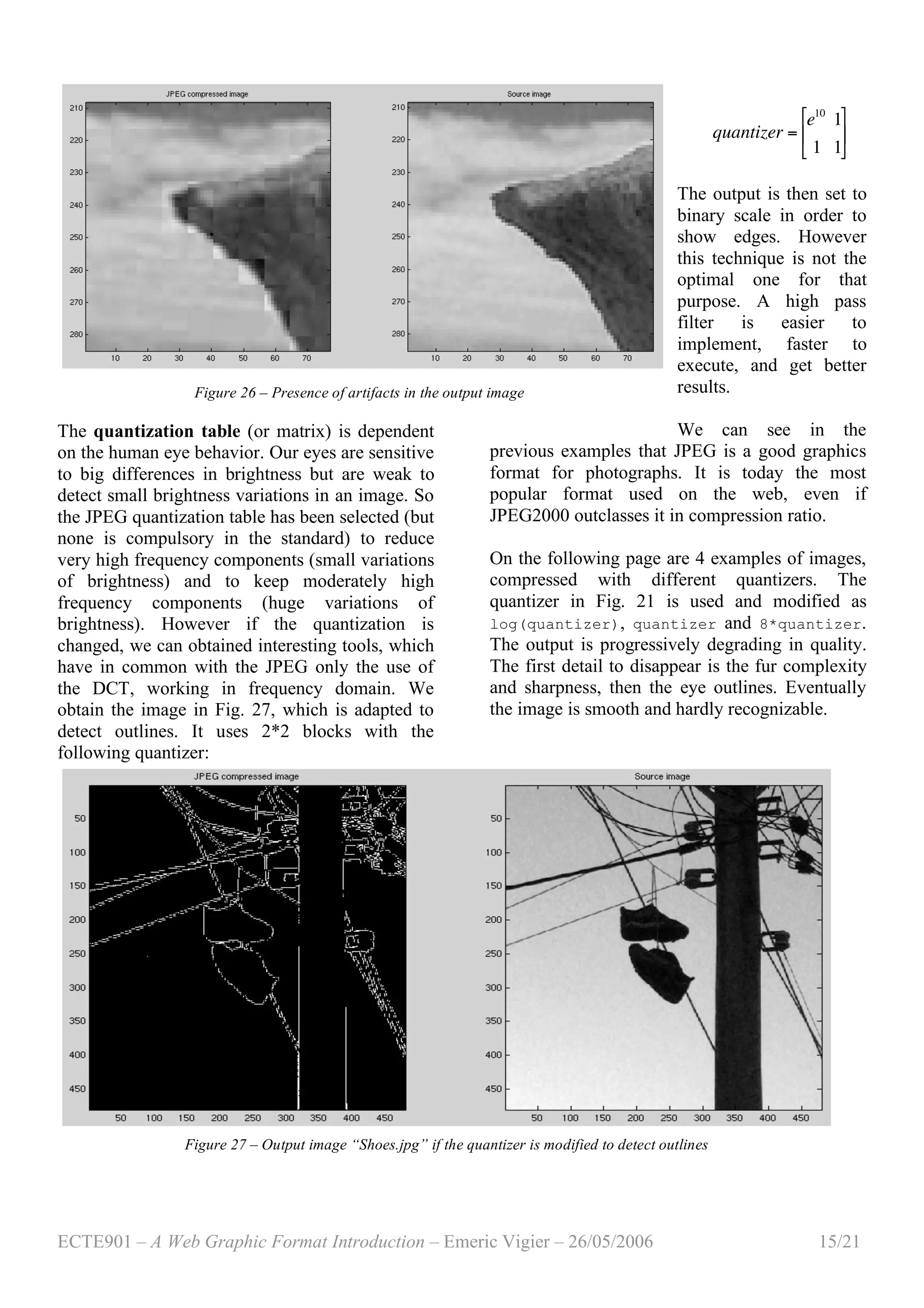
Figure 16 – Binary Transparency issue on a grayscale
image. The algorithm keeps the gray pixels opaque
PNG supports palette-based images with
transparency called cheap transparency. In
comparison, GIF format only supports binary
transparency, which can results in problems
shown in Fig.16 if the background color is not
white. In binary transparency, only a single
palette color (also palette entry) is marked at
completely transparent, all others are fully
opaque. PNG also supports Alpha channel, which
is more byte consuming (double the image bytes
for grayscale). As seen in the table of Fig. 14,
only 8 and 16 bit images can receive an alpha
channel.
2.2.3 Filtering
Before the image is compressed with the
DEFLATE algorithm, it can be filtered to
improve the efficiency of the later compression.
PNG uses 4 kinds of different filters:
 NONE – Each byte is
unchanged, the scanline is
transmitted unmodified;
 SUB – Each byte is replaced by
the difference between its
value and its predecessor on
the left (similar to DC
coefficient encoding in JPEG);
 UP – Here each byte is
replaced by the difference with
its predecessor above it,
 AVERAGE - Each byte is
replaced with the difference
between it and the average of
the corresponding bytes to its
left and above it, truncating any fractional
part,
 PAETH - Each byte is replaced with the
difference between it and the Paeth predictor
of the corresponding bytes to its left, above it,
and to its upper left.
Filtering operates on bytes, not on pixels. It
means that the filter can work on more than one
pixel at a time if the chosen palette is less than 8
bits. This approach improves the efficiency of
decoders by avoiding bit-level manipulations
[18]. Also if the image includes an alpha channel,
image data and alpha data are filtered in the same
way. If the interleaving process is used, each pass
is encoded as a common image. The filter will
select the previously transmitted scanline instead
of the adjacent one in the full image. The
interleaving operation will be seen later in this
study. In any filter, the first byte filtered is always
considering the byte on its left as equal to zero.
And if the reference is the scanline above, the
whole scanline will be considered as null. Filters
perform differently depending on the image type,
thus PNG does not impose a kind of filter to use.
Invented by Alan Paeth, the Paeth predictor is
computed by first calculating a base value, equal
to the sum of the corresponding bytes to the left
Figure 15 – Compositing image operations

and above, minus the byte to the upper left. In the
formula above, “x ranges from zero to the number
of bytes representing the scanline minus one,
Raw(x) refers to the raw data byte at that byte
position in the scanline, Prior(x) refers to the
unfiltered bytes of the prior scanline, and bpp is
defined as for the Sub filter” [18]. The
Paethpredictor is chosen as the adjacent pixel
with the closest value to the one computed inside
the parentheses.
2.2.4 Deflate Compression
PNG implements the Deflate algorithm to
compress images. Deflate is a compression
algorithm, which has been derived form LZ77
(used in zip, gzip, pkzip) and Huffman Coding.
Contrary to the LZW used by the GIF format,
Deflate is patent-free. LZ77 works on a sliding
window. When reading a file, a current position
pointer is moved along the elements. The sliding
window is denoting a memory of these previous
elements passed by this pointer. It is called a
dictionary. An image is a stream of characters (or
numbers), representing pixel values. Instead of
coding each character directly, Deflate has first a
look to previous iterations of this string in the
sliding window. If it matches the same string, it
will code the current string with a pair of
numbers:
 The first denoting the size of the string,
 The second measuring the distance back to
the previous iteration of the string.
Longer is the string, better is the compression, as
it will save the encoding of many characters. If
the current character does not match any character
in the dictionary, the algorithm codes the
unmatched character as normal (e.g. ASCII).
That means that the decoder must be able to do
the difference between ordered pairs
(compressed) and characters coded normally
(unmatched, not compressed). It infers that the
coder transmit a kind of overhead for unmatched
characters, which causes expansion (coding this
character takes more space than without
compression). Therefore the size of the dictionary
and the possible lookahead
is critical to the
compression rate.
The Deflate compression uses this LZ77 method
to compress data and then implements Huffman
coding. It means that Deflate compresses LZ77
output with Huffman coding, which is already
compressed. The Huffman coding has already
been discussed in 2.1.5.
2.2.5 Interlacing
Interlacing is used to show a low definition
preview of the image before the download
completes. This is a particularly interesting
feature for the Web as it allows the user to decide
to continue the download or not. Today’s
connection speed makes most of the images
appear instantaneously but pictures are increasing
in size (e.g. GoogleMap, Flick’r), thus the
interlacing should still be useful. Most of the
pictures on today’s websites are displayed as they
are received. They appear top to bottom as the
download is running. The JPEG uses this method.
Adam7 is a 2D-interlacing scheme, compare to
the 1D-scheme used by GIF. This latter format is
using 4 passes to represent the image, whereas
PNG uses 7 passes. The first pass shows 1/64th
of
the image, thus taking 1/64th
of the download time
to appear on the user screen. This image shown
here will be rough but can offer an interesting
preview. Also the web browser can use
interpolation (bilinear or bicubic) to smooth the
pixels. Interpolation predicts pixels in between
given pixels. It is a commonly used method in
rendering in 3D video games. Using this method,
an interlaced PNG image is split into 7
subimages, as represented in Fig. 17. The
subimages are stored in the PNG file in numerical
order. Note that this method slightly increases the
PNG file size.
!
Paeth x( ) = Raw x( )" Paethpredictor Raw x " bpp( ), prior x( ), prior x " bpp( )( )

Figure 17 – 8*8 pattern of the image split in 7 sections
With 1/64th
of the data, the GIF format is showing
the top of the image, it has not really started the
interlacing yet, it started the first pass at least. The
first GIF interlacing pass will complete after 1/8th
of the image is received. At this time, the PNG
will be at its 4th
pass. Let us have a look on Fig.
18, 19 and 19 [15].
Figure 18 – First PNG interlacing pass, 1/64th
of the full
image received. From left to right, top to bottom: Bicubic
PNG, Bilinear PNG, Interlaced PNG, and Interlaced GIF
Figure 19 – 3rd
PNG interlacing pass, halfway of the 1st
GIF
pass. 1/16th
of the information received. From left to right,
top to bottom: Bicubic PNG, Bilinear PNG, Interlaced
PNG, and Interlaced GIF
Figure 20 – 4th
PNG interlacing pass, 1st
GIF pass. From
left to right, top to bottom: Bicubic PNG, Bilinear PNG,
Interlaced PNG, and Interlaced GIF
The PNG Adam7 interlacing method is already
showing a blocky image with only 1/64th
of the
total information. The PNG will complete a
second pass with 1/32th, a third one with 1/16th
and a fourth one with 1/8th
of the image
information. It progressively becomes clearer and
clearer until the total image has been downloaded.

The point is that PNG draw a much better preview
of the image than GIF does.
However this method is not very popular on the
web, as PNG was not designed to display
photographs. People prefer using the JPEG
format, reducing the image size rather than
displaying a large lossless image in several
passes. And using interlacing with text or sharp
transition images is not really useful since these
images are usually small and are downloaded
quickly. Nonetheless, for very large pictures,
which are transmitted line by line, the interlacing
should be used. However as large pictures refers
usually to photographic pictures, the JPEG format
is often chosen to display them instead of the
PNG because the compression is better. Most of
the time, the website shows the image in a JPEG
thumbnail (smaller copy) for preview and the user
can download the full JPEG image if the preview
fits his needs. A better use of interlacing should
be in movies, where the download process is long
(even with large bandwidth), to show a preview of
the whole sequence while the download is
completing. This method is also used when the
movie is played back or forward to display the
current image without consuming a lot of
resources.
3 Implementation
3.1 JPEG
In this part, an essay of implementing the
JPEG transform and quantizer on Matlab is
carried out. The results will be compared and
displayed as well as the *.m source code. Many
free software and/or libraries can be found and
download on the web but no one will be discussed
here. The program discussed is using two Matlab
functions: cosmat.m and JPEGprogram.m (see
appendix for the program code). The former
function is returning an N*N DCT-II matrix. The
latter program implements the JPEG steps seen in
theory:
 Divide the source image into 8*8 pixel blocks
 Shift each pixel value to range in [-128, 127]
 Convert each block in frequency domain
using the DCT-II transform
 Reduce the information by quantizing each
DCT block.
The decoder is running the same steps in reverse
order to retrieve the source image in a lossy
format. For simplicity, the color space
transformation and downsampling are not
processed in the program. It means that the color
result will not be discussed here. Actually only
grayscale images samples will be tested in this
part. The function converting the RGB color
space to YCbCr is given in annex. Moreover the
Huffman coding will not be treated here, it means
that the file size will not be discussed. What will
be discussed in this part is the role of the
quantization table in the output image quality.
The program uses the special feature of the DCT-
II:
!
C"1
= CT
y8*8 = C # x8*8 # CT
x8*8 = CT
# y8*8 # C
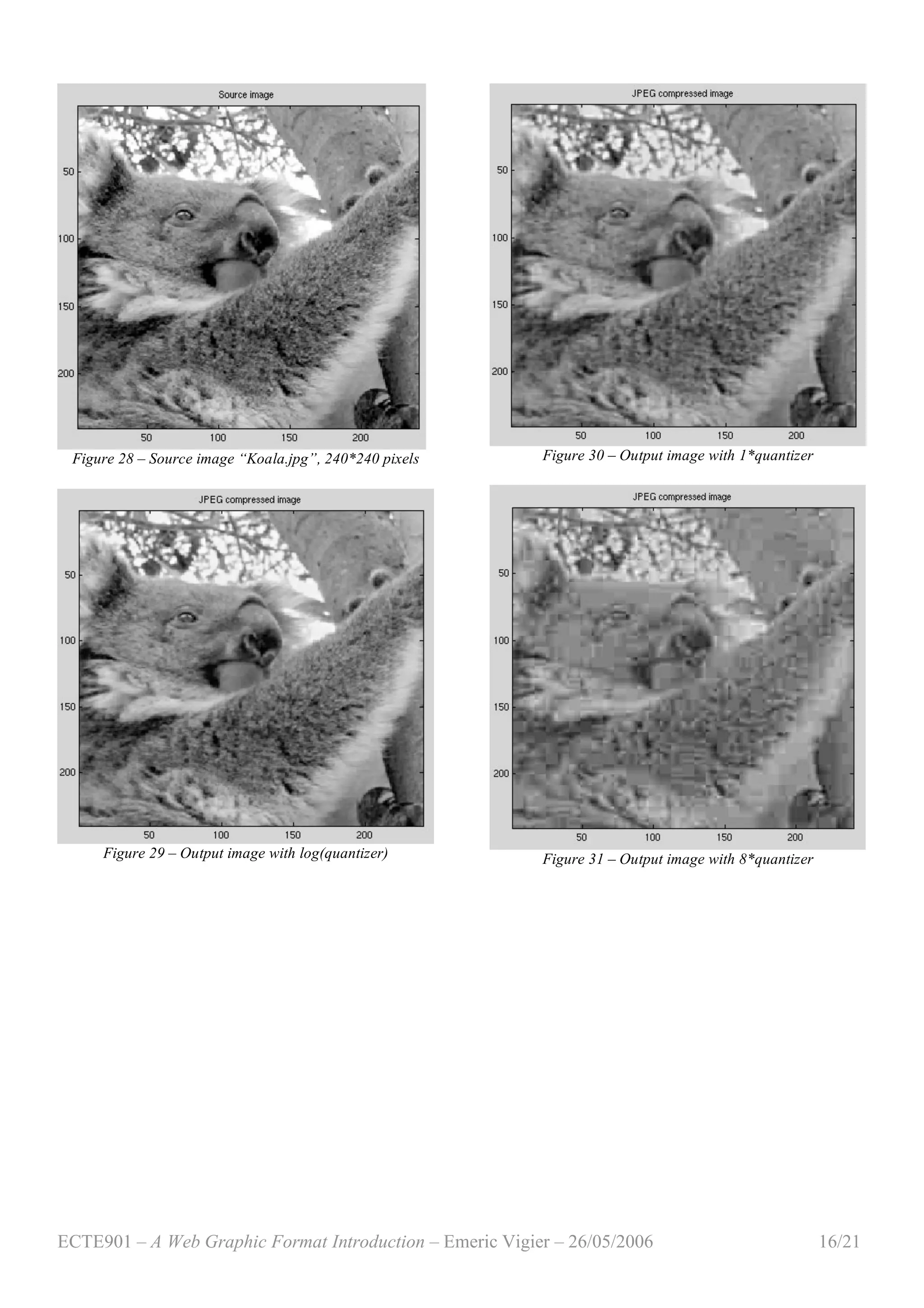
Several quantization matrices are tested and the
results are given in the following figures. The
source image Rocks480.jpg is a sRGB
(IEC61966-2.1) image of 480*480 pixels with a
bit depth of 8 bits. It is taking 324 KBytes space
with a real file size of 255,300 bytes. It is
converted into grayscale by Matlab then
transformed. The quantization matrix used is:
Figure 21 – Quantization matrix
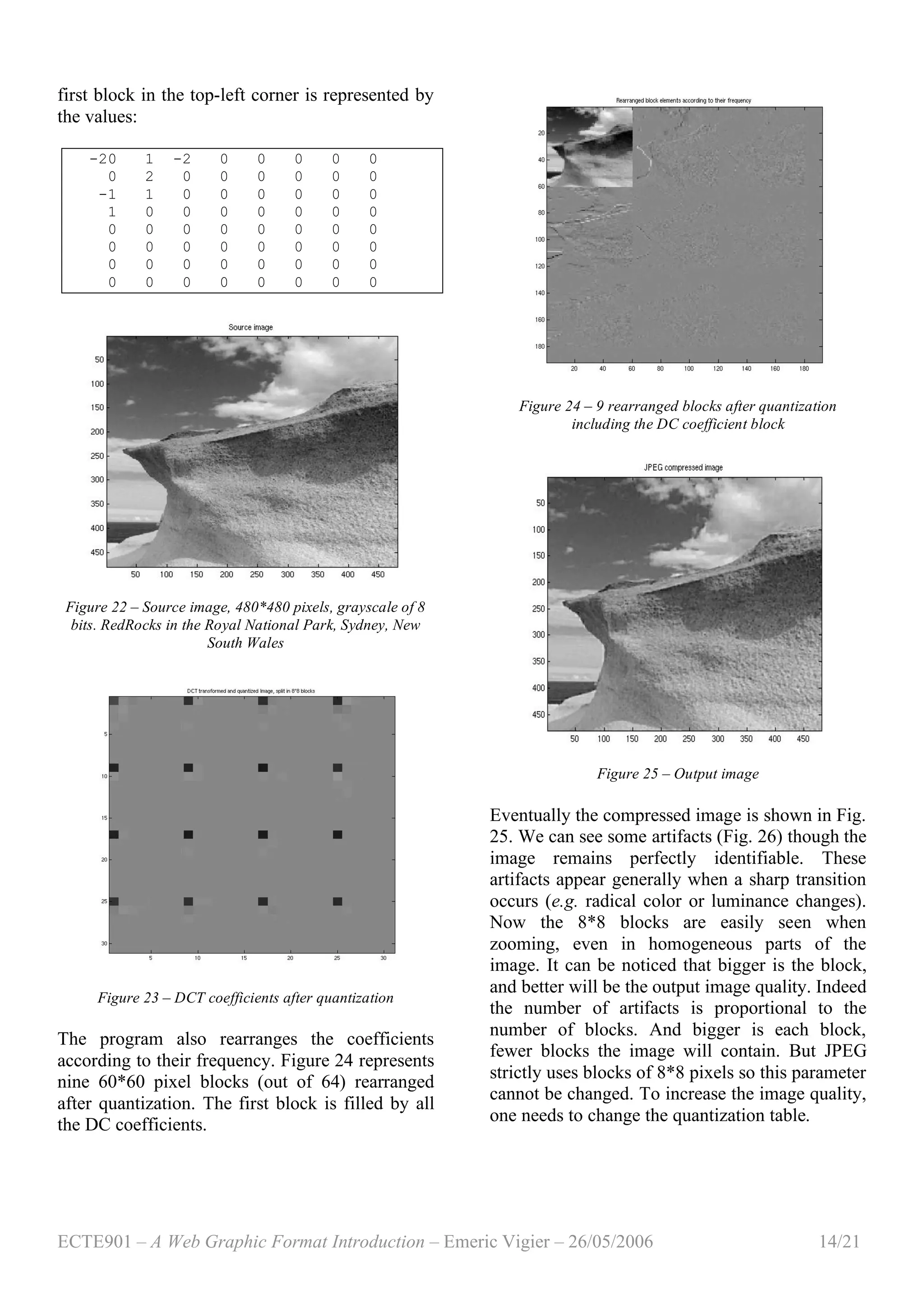
After processing the DCT-II and quantization, a
matrix of coefficients can be observed. The
quantizer makes most of the high frequency
coefficients (in the bottom-right corner) of each
block equal to zero (Fig. 23). For example, the

first block in the top-left corner is represented by
the values:
-20 1 -2 0 0 0 0 0
0 2 0 0 0 0 0 0
-1 1 0 0 0 0 0 0
1 0 0 0 0 0 0 0
0 0 0 0 0 0 0 0
0 0 0 0 0 0 0 0
0 0 0 0 0 0 0 0
0 0 0 0 0 0 0 0
Figure 22 – Source image, 480*480 pixels, grayscale of 8
bits. RedRocks in the Royal National Park, Sydney, New
South Wales
Figure 23 – DCT coefficients after quantization
The program also rearranges the coefficients
according to their frequency. Figure 24 represents
nine 60*60 pixel blocks (out of 64) rearranged
after quantization. The first block is filled by all
the DC coefficients.
Figure 24 – 9 rearranged blocks after quantization
including the DC coefficient block
Figure 25 – Output image
Eventually the compressed image is shown in Fig.
25. We can see some artifacts (Fig. 26) though the
image remains perfectly identifiable. These
artifacts appear generally when a sharp transition
occurs (e.g. radical color or luminance changes).
Now the 8*8 blocks are easily seen when
zooming, even in homogeneous parts of the
image. It can be noticed that bigger is the block,
and better will be the output image quality. Indeed
the number of artifacts is proportional to the
number of blocks. And bigger is each block,
fewer blocks the image will contain. But JPEG
strictly uses blocks of 8*8 pixels so this parameter
cannot be changed. To increase the image quality,
one needs to change the quantization table.

The quantization table (or matrix) is dependent
on the human eye behavior. Our eyes are sensitive
to big differences in brightness but are weak to
detect small brightness variations in an image. So
the JPEG quantization table has been selected (but
none is compulsory in the standard) to reduce
very high frequency components (small variations
of brightness) and to keep moderately high
frequency components (huge variations of
brightness). However if the quantization is
changed, we can obtained interesting tools, which
have in common with the JPEG only the use of
the DCT, working in frequency domain. We
obtain the image in Fig. 27, which is adapted to
detect outlines. It uses 2*2 blocks with the
following quantizer:
!
quantizer =
e10
1
1 1
"
#
$
%
&
'
The output is then set to
binary scale in order to
show edges. However
this technique is not the
optimal one for that
purpose. A high pass
filter is easier to
implement, faster to
execute, and get better
results.
We can see in the
previous examples that JPEG is a good graphics
format for photographs. It is today the most
popular format used on the web, even if
JPEG2000 outclasses it in compression ratio.
On the following page are 4 examples of images,
compressed with different quantizers. The
quantizer in Fig. 21 is used and modified as
log(quantizer), quantizer and 8*quantizer.
The output is progressively degrading in quality.
The first detail to disappear is the fur complexity
and sharpness, then the eye outlines. Eventually
the image is smooth and hardly recognizable.
Figure 27 – Output image “Shoes.jpg” if the quantizer is modified to detect outlines
Figure 26 – Presence of artifacts in the output image

Figure 28 – Source image “Koala.jpg”, 240*240 pixels
Figure 29 – Output image with log(quantizer)
Figure 30 – Output image with 1*quantizer
Figure 31 – Output image with 8*quantizer

CONCLUSION
Web graphic formats strongly implemented
today are still JPEG and GIF. However GIF is
being slowly replaced by the PNG even if PNG’s
popularity still needs to rise up (browser complete
support, public awareness…). PNG is the perfect
example of the format, which tried to replace an
older one by providing higher features but without
responding to a real need. GIF worked well and
PNG was only a minor improvement. However a
key of PNG is the patent freedom, which is
enough to adopt it.
JPEG is still a very good standard for photographs
and did a very nice job before the arrival of
JPEG2000, which is beginning to appear on the
web.
Websites required fast image display, thus high
compression and interlacing algorithms.
Nowadays, bandwidths are huge, even for public
consumption, and pictures are becoming really
large (several Mbytes). Displaying images is no
longer a problem with the strong implementation
of supported formats.
Today’s issue is turned on providing fast
downloads, useful previews and high quality
movies with compression formats such as MPEG-
4. This field is more expected to be subject to
major improvements on web standards and
application supports.

APPENDIX
[1] Matlab program: cosmat.m
% cosmat.m
% Emeric Vigier, University Of Wollongong
% May 2006
% Returns the N*N DCT-II matrix
function C = cosmat(N);
k = 0;
while (k < N)
n = 0;
while (n < N)
if (k == 0)
gamma = 1./sqrt(2);
else
gamma = 1;
end;
C(k+1,n+1) = sqrt(2./N) .* gamma .* cos((k.*(n+1./2).*pi)./N);
n = n+1;
end;
k = k+1;
end;
[2] Matlab program: rgb2ycbcr.m
function T_YCbCr=rgb2ycbcr(T)
imageR=T(:,:,1);
imageV=T(:,:,2);
imageB=T(:,:,3);
T_YCbCr(:,:,1)=0.257*imageR+0.504*imageV+0.098*imageB+16;
T_YCbCr(:,:,2)=-0.148*imageR-0.291*imageV+0.439*imageB+128;
T_YCbCr(:,:,3)=0.439*imageR-0.368*imageV+0.071*imageB+128;
[3] Matlab program: JPEGprogram.m
% JPEGprogram.m
% Emeric Vigier, University Of Wollongong
% May 2006
% Compresses an square grayscale image in a close to JPEG format
clear all;
blockSize = 8;
C = cosmat(blockSize);
X = imread('RedRocks480.jpg');
sourceImage = double(X(:,:,1));
imageSize = length(sourceImage);
% sourceImage is a picture of 480*480px
figure(1)
% display the image in b&w
imagesc(sourceImage);

colormap(gray(256));
title('Source image');
% cell of 3600 8*8-matrices
myYCell = cell(imageSize/blockSize);
quantizer = [ 16 11 10 16 24 40 51 61;...
12 12 14 19 26 58 60 55;...
14 13 16 24 40 57 69 56;...
14 17 22 29 51 87 80 62;...
18 22 37 56 68 109 103 77;...
24 35 55 64 81 104 113 92;...
49 64 78 87 103 121 120 101;...
72 92 95 98 112 100 103 99 ];
% Shifting the pixel values
sourceImage = sourceImage - 128;
% Computing the 2-D DCT for each block and rounding to the nearest integer
for (i = 0:imageSize/blockSize-1)
for (j = 0:imageSize/blockSize-1)
% myYCell{i+1,j+1} =
round(DCTviaFFT(sourceImage(blockSize*i+1:blockSize*(i+1),blockSize*j+1:blockSize*(j+
1))));
myYCell{i+1,j+1} = round(C *
sourceImage(blockSize*i+1:blockSize*(i+1),blockSize*j+1:blockSize*(j+1)) * C');
% Quantizing each block
myYCell{i+1, j+1} = round(myYCell{i+1, j+1} ./ quantizer);
end;
end;
myRearrangedYCell = cell(blockSize); % cell of 64 60*60-matrices
% Rearranging blocks and quantizing
for (blockRowCounter = 1:blockSize) % from 1 to 8
for (blockColumnCounter = 1:blockSize)
for (i = 1:imageSize/blockSize) % from 1 to 60, loop on myBlock60by60 rows
for(j = 1:imageSize/blockSize)
myBlock8by8 = myYCell{i,j};
myBlock60by60(i,j) = myBlock8by8(blockRowCounter,blockColumnCounter);
end;
end;
myRearrangedYCell{blockRowCounter,blockColumnCounter} = myBlock60by60;
end;
end;
myRearrangedY = cell2mat(myRearrangedYCell);
figure(2)
imagesc(cell2mat(myYCell));
title('DCT transformed and quantized Image, split in 8*8 blocks');
figure(3)
imagesc(myRearrangedY);
title('Rearranged block elements according to their frequency');

% Reconstructing x from y without error
for (i = 1:imageSize/blockSize) % from 1 to 60, loop on myBlock60by60 rows
for(j = 1:imageSize/blockSize)
for (blockRowCounter = 1:blockSize) % from 1 to 8
for (blockColumnCounter = 1:blockSize)
myBlock60by60 =
myRearrangedYCell{blockRowCounter,blockColumnCounter};
myBlock8by8(blockRowCounter,blockColumnCounter) = myBlock60by60(i,j);
end;
end;
myReconstructedYCell{i,j} = myBlock8by8;
end;
end;
myReconstructedY = cell2mat(myReconstructedYCell);
for (i = 0:imageSize/blockSize-1)
for (j = 0:imageSize/blockSize-1)
myReconstructedY(blockSize*i+1:blockSize*(i+1),blockSize*j+1:blockSize*(j+1))
= ...
myReconstructedY(blockSize*i+1:blockSize*(i+1),blockSize*j+1:blockSize*(j+1)) .*
quantizer;
myReconstructedX(blockSize*i+1:blockSize*(i+1),blockSize*j+1:blockSize*(j+1))
= ...
C' * myReconstructedYCell{i+1,j+1} * C;
end;
end;
myReconstructedX = myReconstructedX + 128;
figure(4)
subplot(1,2,1);
imagesc(myReconstructedX);
title('JPEG compressed image');
subplot(1,2,2);
imagesc(sourceImage);
title('Source image');

REFERENCES
[1] O. L. Astrachan, Huffman Coding, a CS2
Assignment, unpublished, 2004.
http://www.cs.duke.edu/csed/poop/huff/info
[2] Fast Fourier Transform, BookRags
http://www.bookrags.com/sciences/computerscience/
fast-fourier-transform-wcs.html
[3] JPEG, MPEG, BookRags, 2006.
http://www.bookrags.com/sciences/computerscience/
jpeg-mpeg-csci-02.html
[4] T. Boutell et al., “PNG (Portable Network
Graphics) Specification”, W3C
Recommendation, October 1996.
http://www.libpng.org/pub/png/
[5] C. M. Brislawn, The FBI Fingerprint Image
Compression Standard
http://www.c3.lanl.gov/~brislawn/FBI/FBI.html
[6] S. Cavanaugh, “To PNG or not to PNG”,
unpublished, EyeWire.
http://www.eyewire.com/magazine/columns/sean
[7] “Digital Compression and Coding of
Continuous-tone Still Images, ISO/IEC
10918-1”, CCITT/ITU, 1992.
[8] B. V. Dasarathy, Image Data Compression,
IEEE Computer Society Press, 1995.
[9] V. K. Goyal, “Theorical Foundations of
Transform Coding”, IEEE Signal
Processing Magazine, September 2001.
[10] E. Hamilton, “JPEG File Interchange
Format”, C-Cube Microsystems, 1992.
[11] D. Hankerson, G. A. Harris, P. D. Johnson
Jr., “Introduction to Information Theory and
Data Compression”, Chapman & Hall/CRC,
2003.
[12] D. A. Huffman, “A Method of the
Construction of Minimum-Redundancy
Codes”, I.R.E., pp. 1098-1102, September
1952.
[13] JPEG Homepage, Joint Photographic
Expert Group, 2004.
http://www.jpeg.org/jpeg/index.html
[14] S. A. Khayam, “The Discrete Cosine
Transform, theory and application”,
unpublished, Michigan State University,
2003.
[15] S. T. Lavavej, “Introduction to PNG”,
unpublished
http://nuwen.net/png.html
[16] A. Leger, T. Omachi and G. K. Wallace,
“JPEG Still Picture Compression
Algorithm”, Optical Engineering, Vol. 30,
No. 7, pp. 947-954, 1991.
[17] W. B. Pennebaker, J. L. Mitchell, JPEG
Still Image Data Compression Standard,
Van Nostrand Reinhold, 1993.
[18] G. Roelofs, PNG: The definitive Guide,
O’Reilly & Associates, 1999.
[19] A. Skodras, C. Christopoulos, T. Ebrahimi,
“The JPEG 2000 Still Image Compression
Standard”, IEEE Signal Processing
Magazine, September 2001.
[20] Chroma Subsampling, Wikipedia, 2006.
http://en.wikipedia.org/wiki/YUV_4:4:4
[21] Deflate, Wikipedia, 2006.
http://en.wikipedia.org/wiki/DEFLATE
[22] GIF, Wikipedia, 2006.
http://en.wikipedia.org/wiki/Gif
[23] Huffman Coding, Wikipedia, 2006.
http://en.wikipedia.org/wiki/Huffman_coding
[24] LZW, Wikipedia, 2006.
http://en.wikipedia.org/wiki/LZW
[25] PNG, Wikipedia, 2006.
http://en.wikipedia.org/wiki/Png
[26] Wavelet, Wikipedia, 2006.
http://en.wikipedia.org/wiki/Wavelet

ECTE901_AssignmentReport_v1.2

Recommended

Recommended

More Related Content

Viewers also liked

Viewers also liked (16)

Similar to ECTE901_AssignmentReport_v1.2

Similar to ECTE901_AssignmentReport_v1.2 (20)

ECTE901_AssignmentReport_v1.2