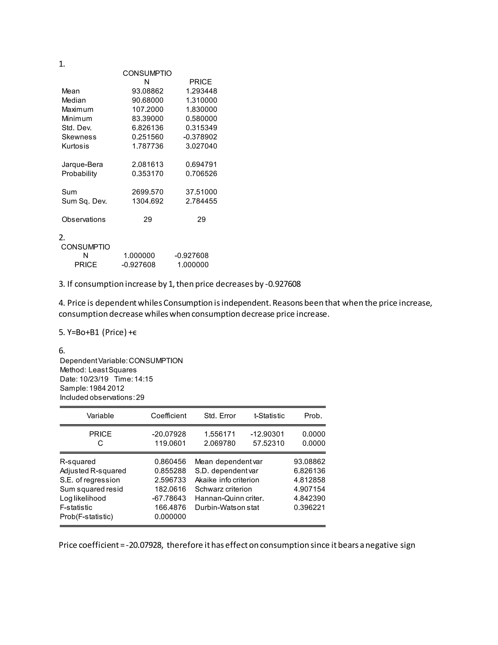
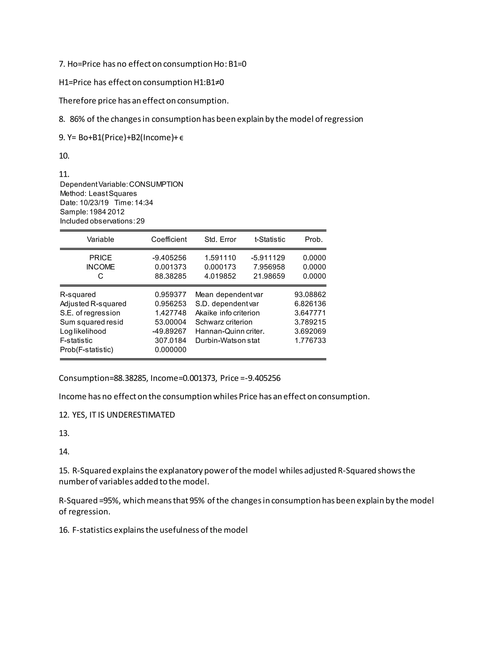
This document analyzes the relationship between consumption and price using statistical analysis and regression models. It finds: 1. There is a strong negative correlation between consumption and price, meaning as price increases consumption decreases. 2. A regression model with price as the independent variable explains 86% of the changes in consumption. 3. Adding income as a second independent variable improves the model fit, with price and income both having a statistically significant impact on consumption.

1. 1.
CONSUMPTIO
N PRICE
Mean 93.08862 1.293448
Median 90.68000 1.310000
Maximum 107.2000 1.830000
Minimum 83.39000 0.580000
Std. Dev. 6.826136 0.315349
Skewness 0.251560 -0.378902
Kurtosis 1.787736 3.027040
Jarque-Bera 2.081613 0.694791
Probability 0.353170 0.706526
Sum 2699.570 37.51000
Sum Sq. Dev. 1304.692 2.784455
Observations 29 29
2.
CONSUMPTIO
N 1.000000 -0.927608
PRICE -0.927608 1.000000
3. If consumptionincrease by1,thenprice decreasesby -0.927608
4. Price is dependentwhilesConsumptionisindependent.Reasonsbeenthat when the price increase,
consumptiondecrease whileswhenconsumptiondecrease price increase.
5. Y=Bo+B1 (Price) +ϵ
6.
DependentVariable:CONSUMPTION
Method: LeastSquares
Date: 10/23/19 Time:14:15
Sample:1984 2012
Included observations:29
Variable Coefficient Std. Error t-Statistic Prob.
PRICE -20.07928 1.556171 -12.90301 0.0000
C 119.0601 2.069780 57.52310 0.0000
R-squared 0.860456 Mean dependentvar 93.08862
Adjusted R-squared 0.855288 S.D. dependentvar 6.826136
S.E. of regression 2.596733 Akaike info criterion 4.812858
Sum squared resid 182.0616 Schwarz criterion 4.907154
Log likelihood -67.78643 Hannan-Quinn criter. 4.842390
F-statistic 166.4876 Durbin-Watson stat 0.396221
Prob(F-statistic) 0.000000
Price coefficient=-20.07928, therefore ithaseffectonconsumptionsince itbearsanegative sign

2. 7. Ho=Price hasno effectonconsumptionHo:B1=0
H1=Price has effectonconsumptionH1:B1≠0
Therefore price hasaneffectonconsumption.
8. 86% of the changesin consumptionhasbeenexplainbythe model of regression
9. Y= Bo+B1(Price)+B2(Income)+ϵ
10.
11.
DependentVariable:CONSUMPTION
Method: LeastSquares
Date: 10/23/19 Time:14:34
Sample:1984 2012
Included observations:29
Variable Coefficient Std. Error t-Statistic Prob.
PRICE -9.405256 1.591110 -5.911129 0.0000
INCOME 0.001373 0.000173 7.956958 0.0000
C 88.38285 4.019852 21.98659 0.0000
R-squared 0.959377 Mean dependentvar 93.08862
Adjusted R-squared 0.956253 S.D. dependentvar 6.826136
S.E. of regression 1.427748 Akaike info criterion 3.647771
Sum squared resid 53.00004 Schwarz criterion 3.789215
Log likelihood -49.89267 Hannan-Quinn criter. 3.692069
F-statistic 307.0184 Durbin-Watson stat 1.776733
Prob(F-statistic) 0.000000
Consumption=88.38285, Income=0.001373, Price =-9.405256
Income hasno effectonthe consumptionwhilesPrice hasaneffectonconsumption.
12. YES, IT IS UNDERESTIMATED
13.
14.
15. R-Squaredexplainsthe explanatorypowerof the model whilesadjustedR-Squaredshowsthe
numberof variablesaddedtothe model.
R-Squared=95%, whichmeansthat95% of the changesinconsumptionhasbeenexplainbythe model
of regression.
16. F-statisticsexplainsthe usefulnessof the model