This document provides an overview of data structures and algorithms. It defines data structures as a way to store and organize data for efficient access and updating. There are two main categories of data structures - linear and non-linear. Common linear data structures include arrays and linked lists, while trees and graphs are examples of non-linear data structures. The document also describes common operations for stacks and queues like push, pop, enqueue and dequeue. It concludes by discussing different notations for writing arithmetic expressions like infix, prefix and postfix notations.
![DATA STRUCTURES & ALGORITHMS
UNIT - 1
What are Data Structures?
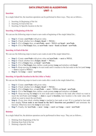
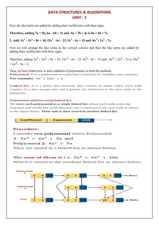
Data structure is a storage that is used to store and organize data. It is a way of arranging data
on a computer so that it can be accessed and updated efficiently.
Depending on your requirement and project, it is important to choose the right data structure
for your project. For example, if you want to store data sequentially in the memory, then you
can go for the Array data structure.
Data structure and data types are slightly different. Data structure is the collection of data
types arranged in a specific order.
Types of Data Structure
Basically, data structures are divided into two categories:
1. Linear data structure
2. Non-linear data structure
Array Representation in Data Structure
Array:
An array defines as a finite ordered set of homogeneous elements. Finite means that there is a specific
number of elements and ordered means that the elements of the array are indexed. Homogeneous means that
all the elements of the array must be of the same type.
Array Representation:
In the Data Structure, there are two types of array representation are exists:
i. One Dimensional Array
ii. Two Dimensional Array
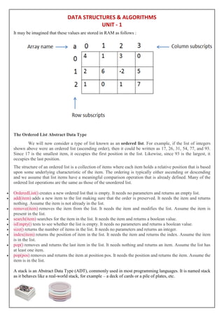
One Dimensional Array:
Values in a mathematical set are written as shown below :
a={5, 7, 9, 4, 6, 8}
These values refer in mathematics as follows :
a0, a1, a2
In Data Structure, these numbers are represented as follows :
a[0], a[1], a[2]
these values are stored in RAM as follows :](https://image.slidesharecdn.com/dsunit1-221110085119-d391d272/85/DS-UNIT-1-pdf-1-320.jpg)
![DATA STRUCTURES & ALGORITHMS
UNIT - 1
What are Data Structures?
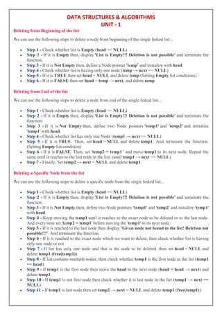
Data structure is a storage that is used to store and organize data. It is a way of arranging data
on a computer so that it can be accessed and updated efficiently.
Depending on your requirement and project, it is important to choose the right data structure
for your project. For example, if you want to store data sequentially in the memory, then you
can go for the Array data structure.
Data structure and data types are slightly different. Data structure is the collection of data
types arranged in a specific order.
Types of Data Structure
Basically, data structures are divided into two categories:
1. Linear data structure
2. Non-linear data structure
Array Representation in Data Structure
Array:
An array defines as a finite ordered set of homogeneous elements. Finite means that there is a specific
number of elements and ordered means that the elements of the array are indexed. Homogeneous means that
all the elements of the array must be of the same type.
Array Representation:
In the Data Structure, there are two types of array representation are exists:
i. One Dimensional Array
ii. Two Dimensional Array
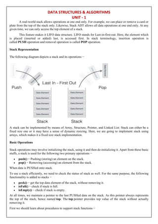
One Dimensional Array:
Values in a mathematical set are written as shown below :
a={5, 7, 9, 4, 6, 8}
These values refer in mathematics as follows :
a0, a1, a2
In Data Structure, these numbers are represented as follows :
a[0], a[1], a[2]
these values are stored in RAM as follows :](https://image.slidesharecdn.com/dsunit1-221110085119-d391d272/75/DS-UNIT-1-pdf-1-2048.jpg)
![DATA STRUCTURES & ALGORITHMS
UNIT - 1
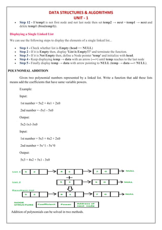
Algorithm for insertion into One-dimensional array:
Algorithm fnInsertion_1D_Array(arrData, n, k, item)
{
for(i=n-1;i>=k-1;i--)
arrData[i+1]=arrData[i];
arrData[k-1]=item;
n=n-1;
} // End of Algorithm
Algorithm for deletion from One-dimensional array:
Algorithm fnDeletion_1D_Array(arrData, n, k)
{
item=arrData[k-1];
for(i=k-1;i<n-1;i++)
arrData[i]=arrData[i+1];
n=n-1;
return item;
} // End of Algorithm
Algorithm for traversing One-dimensional array:
Algorithm fnTraverse_1D_Array(arrData, n)
{
for(i=0;i<n;i++)
print arrData[i];
} //End of Algorithm
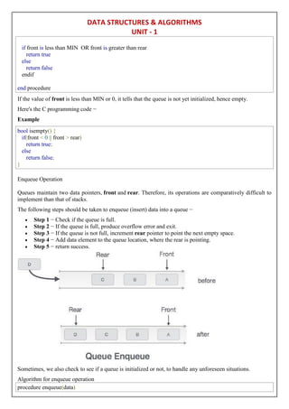
Two Dimensional Array:
These values are referred in mathematical as follows :
A0,0 A0,1 A0,2
In Data Structure, they are represented as follows :
a[0][0] a[0][1] a[0][2] and so on](https://image.slidesharecdn.com/dsunit1-221110085119-d391d272/85/DS-UNIT-1-pdf-2-320.jpg)
![DATA STRUCTURES & ALGORITHMS
UNIT - 1
peek()
Algorithm of peek() function −
begin procedure peek
return stack[top]
end procedure
Implementation of peek() function in C programming language −
Example
int peek() {
return stack[top];
}
isfull()
Algorithm of isfull() function −
begin procedure isfull
if top equals to MAXSIZE
return true
else
return false
endif
end procedure
Implementation of isfull() function in C programming language −
Example
bool isfull() {
if(top == MAXSIZE)
return true;
else
return false;
}
isempty()
Algorithm of isempty() function −
begin procedure isempty
if top less than 1
return true
else
return false
endif
end procedure
Implementation of isempty() function in C programming language is slightly different. We initialize top at -
1, as the index in array starts from 0. So we check if the top is below zero or -1 to determine if the stack is
empty. Here's the code −](https://image.slidesharecdn.com/dsunit1-221110085119-d391d272/85/DS-UNIT-1-pdf-5-320.jpg)
![DATA STRUCTURES & ALGORITHMS
UNIT - 1
Example
bool isempty() {
if(top == -1)
return true;
else
return false;
}
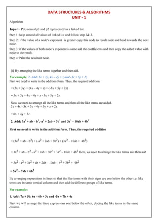
Push Operation
The process of putting a new data element onto stack is known as a Push Operation. Push operation involves
a series of steps −
Step 1 − Checks if the stack is full.
Step 2 − If the stack is full, produces an error and exit.
Step 3 − If the stack is not full, increments top to point next empty space.
Step 4 − Adds data element to the stack location, where top is pointing.
Step 5 − Returns success.
If the linked list is used to implement the stack, then in step 3, we need to allocate space dynamically.
Algorithm for PUSH Operation
A simple algorithm for Push operation can be derived as follows −
begin procedure push: stack, data
if stack is full
return null
endif
top ← top + 1
stack[top] ← data
end procedure
Implementation of this algorithm in C, is very easy. See the following code −
Example
void push(int data) {
if(!isFull()) {](https://image.slidesharecdn.com/dsunit1-221110085119-d391d272/85/DS-UNIT-1-pdf-6-320.jpg)
![DATA STRUCTURES & ALGORITHMS
UNIT - 1
top = top + 1;
stack[top] = data;
} else {
printf("Could not insert data, Stack is full.n");
}
}
Pop Operation
Accessing the content while removing it from the stack, is known as a Pop Operation. In an array
implementation of pop() operation, the data element is not actually removed, instead top is decremented to a
lower position in the stack to point to the next value. But in linked-list implementation, pop() actually
removes data element and deallocates memory space.
A Pop operation may involve the following steps −
Step 1 − Checks if the stack is empty.
Step 2 − If the stack is empty, produces an error and exit.
Step 3 − If the stack is not empty, accesses the data element at which top is pointing.
Step 4 − Decreases the value of top by 1.
Step 5 − Returns success.
Algorithm for Pop Operation
A simple algorithm for Pop operation can be derived as follows −
begin procedure pop: stack
if stack is empty
return null
endif
data ← stack[top]
top ← top - 1
return data
end procedure
Implementation of this algorithm in C, is as follows −
Example](https://image.slidesharecdn.com/dsunit1-221110085119-d391d272/85/DS-UNIT-1-pdf-7-320.jpg)
![DATA STRUCTURES & ALGORITHMS
UNIT - 1
int pop(int data) {
if(!isempty()) {
data = stack[top];
top = top - 1;
return data;
} else {
printf("Could not retrieve data, Stack is empty.n");
}
}
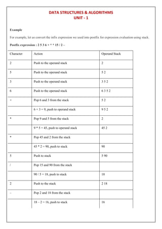
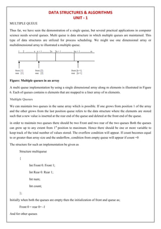
Queue is an abstract data structure, somewhat similar to Stacks. Unlike stacks, a queue is open at both its
ends. One end is always used to insert data (enqueue) and the other is used to remove data (dequeue). Queue
follows First-In-First-Out methodology, i.e., the data item stored first will be accessed first.
A real-world example of queue can be a single-lane one-way road, where the vehicle enters first, exits first.
More real-world examples can be seen as queues at the ticket windows and bus-stops.
Queue Representation
As we now understand that in queue, we access both ends for different reasons. The following diagram
given below tries to explain queue representation as data structure −
As in stacks, a queue can also be implemented using Arrays, Linked-lists, Pointers and Structures. For the
sake of simplicity, we shall implement queues using one-dimensional array.
Basic Operations
Queue operations may involve initializing or defining the queue, utilizing it, and then completely erasing it
from the memory. Here we shall try to understand the basic operations associated with queues −
enqueue() − add (store) an item to the queue.
dequeue() − remove (access) an item from the queue.
Few more functions are required to make the above-mentioned queue operation efficient. These are −
peek() − Gets the element at the front of the queue without removing it.](https://image.slidesharecdn.com/dsunit1-221110085119-d391d272/85/DS-UNIT-1-pdf-8-320.jpg)
![DATA STRUCTURES & ALGORITHMS
UNIT - 1
isfull() − Checks if the queue is full.
isempty() − Checks if the queue is empty.
In queue, we always dequeue (or access) data, pointed by front pointer and while enqueing (or storing) data
in the queue we take help of rear pointer.
Let's first learn about supportive functions of a queue −
peek()
This function helps to see the data at the front of the queue. The algorithm of peek() function is as follows −
Algorithm
begin procedure peek
return queue[front]
end procedure
Implementation of peek() function in C programming language −
Example
int peek() {
return queue[front];
}
isfull()
As we are using single dimension array to implement queue, we just check for the rear pointer to reach at
MAXSIZE to determine that the queue is full. In case we maintain the queue in a circular linked-list, the
algorithm will differ. Algorithm of isfull() function −
Algorithm
begin procedure isfull
if rear equals to MAXSIZE
return true
else
return false
endif
end procedure
Implementation of isfull() function in C programming language −
Example
bool isfull() {
if(rear == MAXSIZE - 1)
return true;
else
return false;
}
isempty()
Algorithm of isempty() function −
Algorithm
begin procedure isempty](https://image.slidesharecdn.com/dsunit1-221110085119-d391d272/85/DS-UNIT-1-pdf-9-320.jpg)
![DATA STRUCTURES & ALGORITHMS
UNIT - 1
if queue is full
return overflow
endif
rear ← rear + 1
queue[rear] ← data
return true
end procedure
Implementation of enqueue() in C programming language −
Example
int enqueue(int data)
if(isfull())
return 0;
rear = rear + 1;
queue[rear] = data;
return 1;
end procedure
Dequeue Operation
Accessing data from the queue is a process of two tasks − access the data where front is pointing and
remove the data after access. The following steps are taken to perform dequeue operation −
Step 1 − Check if the queue is empty.
Step 2 − If the queue is empty, produce underflow error and exit.
Step 3 − If the queue is not empty, access the data where front is pointing.
Step 4 − Increment front pointer to point to the next available data element.
Step 5 − Return success.
Algorithm for dequeue operation
procedure dequeue](https://image.slidesharecdn.com/dsunit1-221110085119-d391d272/85/DS-UNIT-1-pdf-11-320.jpg)
![DATA STRUCTURES & ALGORITHMS
UNIT - 1
if queue is empty
return underflow
end if
data = queue[front]
front ← front + 1
return true
end procedure
Implementation of dequeue() in C programming language −
Example
int dequeue() {
if(isempty())
return 0;
int data = queue[front];
front = front + 1;
return data;
}
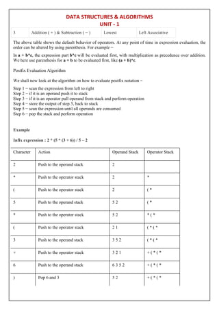
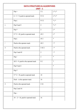
EVALUATION OF EXPRESSIONS
The way to write arithmetic expression is known as a notation. An arithmetic expression can be written in
three different but equivalent notations, i.e., without changing the essence or output of an expression. These
notations are −
Infix Notation
Prefix (Polish) Notation
Postfix (Reverse-Polish) Notation
These notations are named as how they use operator in expression. We shall learn the same here in this
chapter.
Infix Notation
We write expression in infix notation, e.g. a - b + c, where operators are used in-between operands. It is easy
for us humans to read, write, and speak in infix notation but the same does not go well with computing
devices. An algorithm to process infix notation could be difficult and costly in terms of time and space
consumption.
Prefix Notation
In this notation, operator is prefixed to operands, i.e. operator is written ahead of operands. For
example, +ab. This is equivalent to its infix notation a + b. Prefix notation is also known as Polish
Notation.](https://image.slidesharecdn.com/dsunit1-221110085119-d391d272/85/DS-UNIT-1-pdf-12-320.jpg)
![DATA STRUCTURES & ALGORITHMS
UNIT - 1
Prefix expression: – / * 2 * 5 + 3 6 5 2
Reversed prefix expression: 2 5 6 3 + 5 * 2 * / –
Character Action Operand Stack
2 Push to the operand stack 2
5 Push to the operand stack 5 2
6 Push to the operand stack 6 5 2
3 Push to the operand stack 3 6 5 2
+ Pop 3 and 6 from the stack 5 2
3 + 6 = 9, push to operand stack 9 5 2
5 Push to the operand stack 5 9 5 2
* Pop 5 and 9 from the stack 5 2
5 * 9 = 45, push to operand stack 45 5 2
2 Push to operand stack 2 45 5 2
* Pop 2 and 45 from the stack 5 2
2 * 45 = 90, push to stack 90 5 2
/ Pop 90 and 5 from the stack 2
90 / 5 = 18, push to stack 18 2
– Pop 18 and 2 from the stack
18 – 2 = 16, push to stack 16
Data Structure Multiple Stack
A single stack is sometimes not sufficient to store a large amount of data. To overcome this problem, we can
use multiple stack. For this, we have used a single array having more than one stack. The array is divided for
multiple stacks.
Suppose there is an array STACK[n] divided into two stack STACK A and STACK B, where n = 10.
STACK A expands from the left to the right, i.e., from 0th element.
STACK B expands from the right to the left, i.e., from 10th element.
The combined size of both STACK A and STACK B never exceeds 10.](https://image.slidesharecdn.com/dsunit1-221110085119-d391d272/85/DS-UNIT-1-pdf-17-320.jpg)
![DATA STRUCTURES & ALGORITHMS
UNIT - 1
the listen
Why Linked List?
Arrays can be used to store linear data of similar types, but arrays have the following limitations.
The size of the arrays is fixed: So we must know the upper limit on the number of elements in
advance. Also, generally, the allocated memory is equal to the upper limit irrespective of the usage.
Insertion of a new element / Deletion of a existing element in an array of elements is
expensive: The room has to be created for the new elements and to create room existing elements have
to be shifted but in Linked list if we have the head node then we can traverse to any node through it
and insert new node at the required position.
For example, in a system, if we maintain a sorted list of IDs in an array id[].
id[] = [1000, 1010, 1050, 2000, 2040].
And if we want to insert a new ID 1005, then to maintain the sorted order, we have to move all the
elements after 1000 (excluding 1000).
Deletion is also expensive with arrays until unless some special techniques are used. For example, to
delete 1010 in id[], everything after 1010 has to be moved due to this so much work is being done which
affects the efficiency of the code.
Operations on Single Linked List
The following operations are performed on a Single Linked List
Insertion
Deletion
Display
Before we implement actual operations, first we need to set up an empty list. First, perform the following
steps before implementing actual operations.
Step 1 - Include all the header files which are used in the program.
Step 2 - Declare all the user defined functions.
Step 3 - Define a Node structure with two members data and next
Step 4 - Define a Node pointer 'head' and set it to NULL.
Step 5 - Implement the main method by displaying operations menu and make suitable function calls
in the main method to perform user selected operation.](https://image.slidesharecdn.com/dsunit1-221110085119-d391d272/85/DS-UNIT-1-pdf-21-320.jpg)