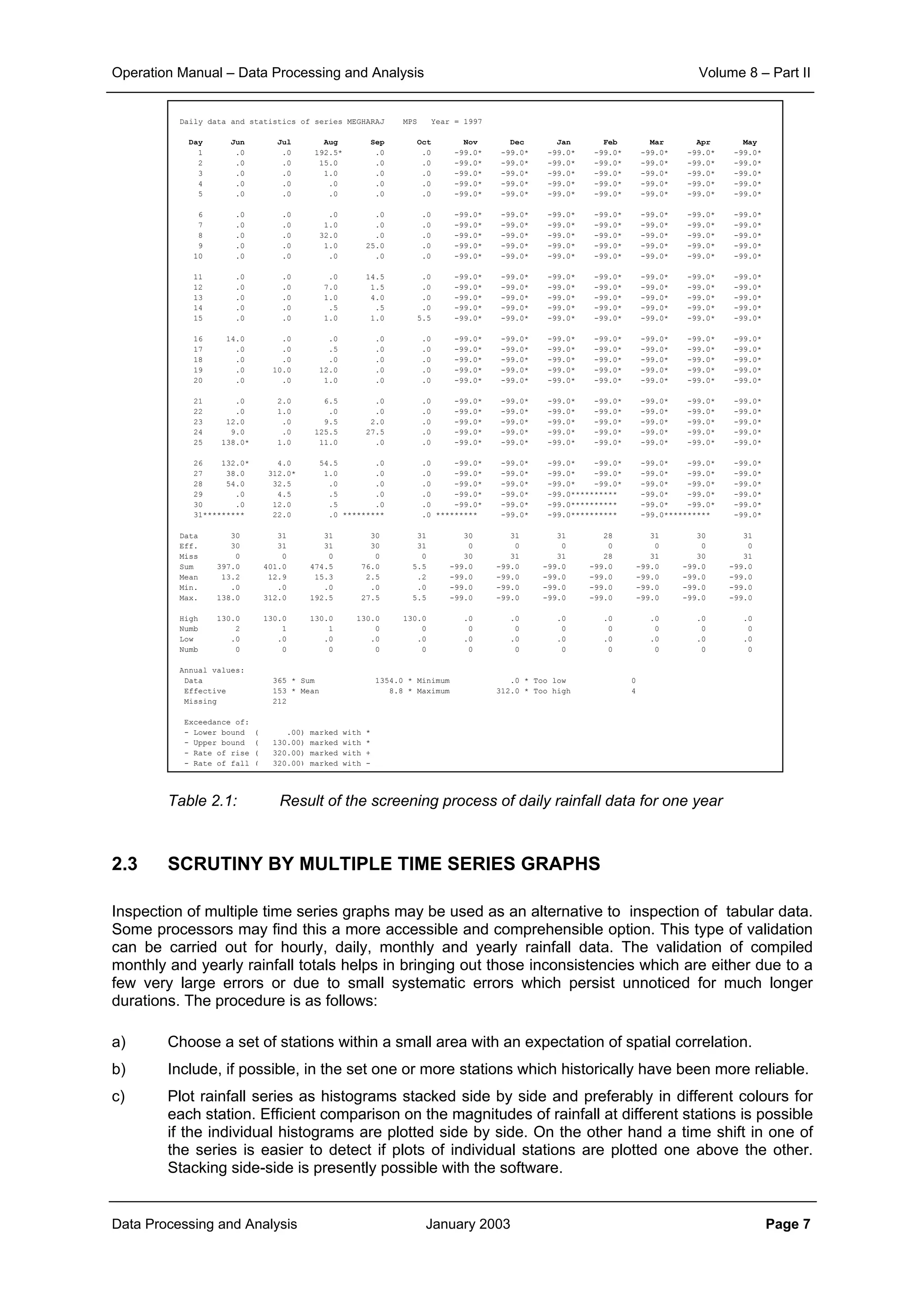
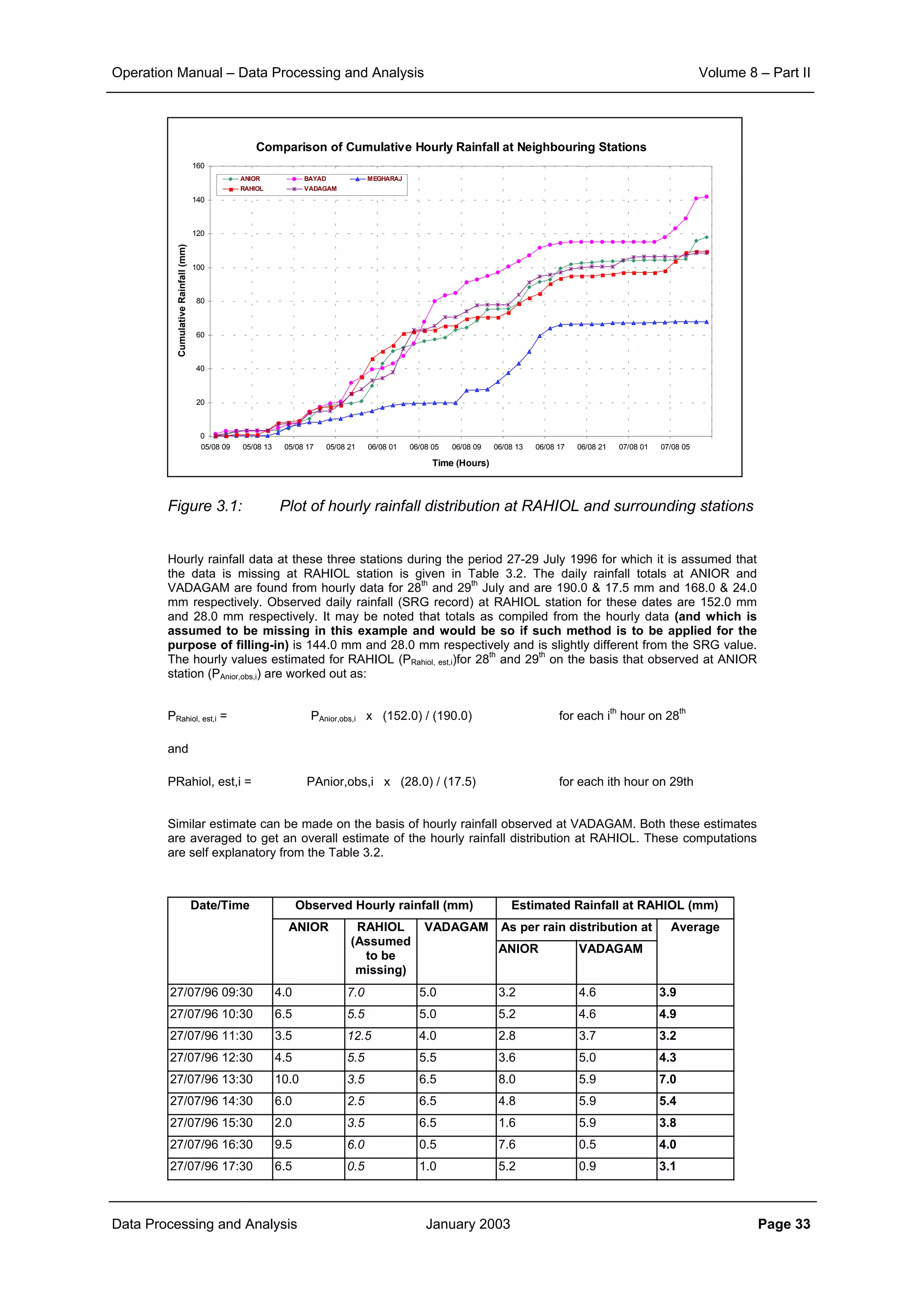
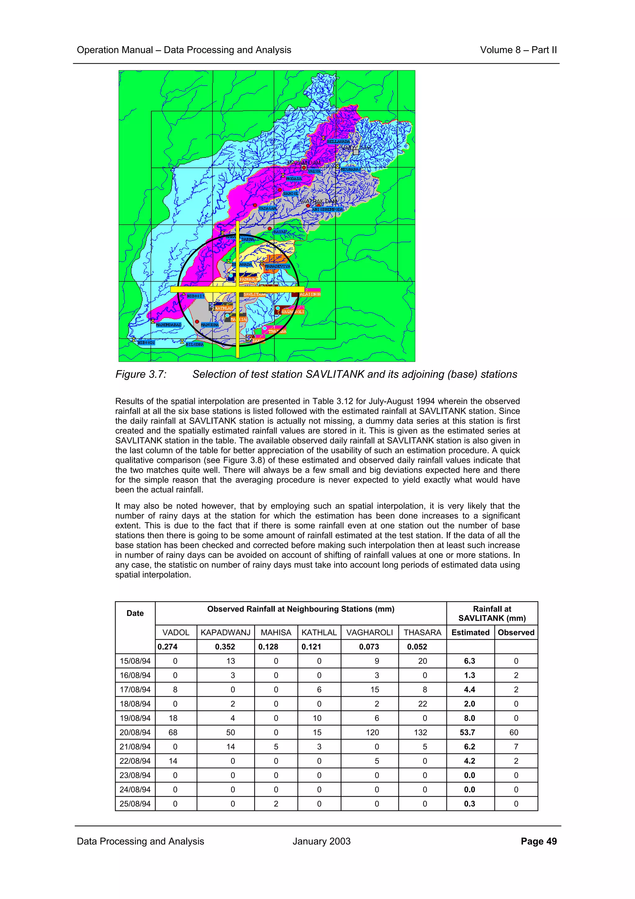
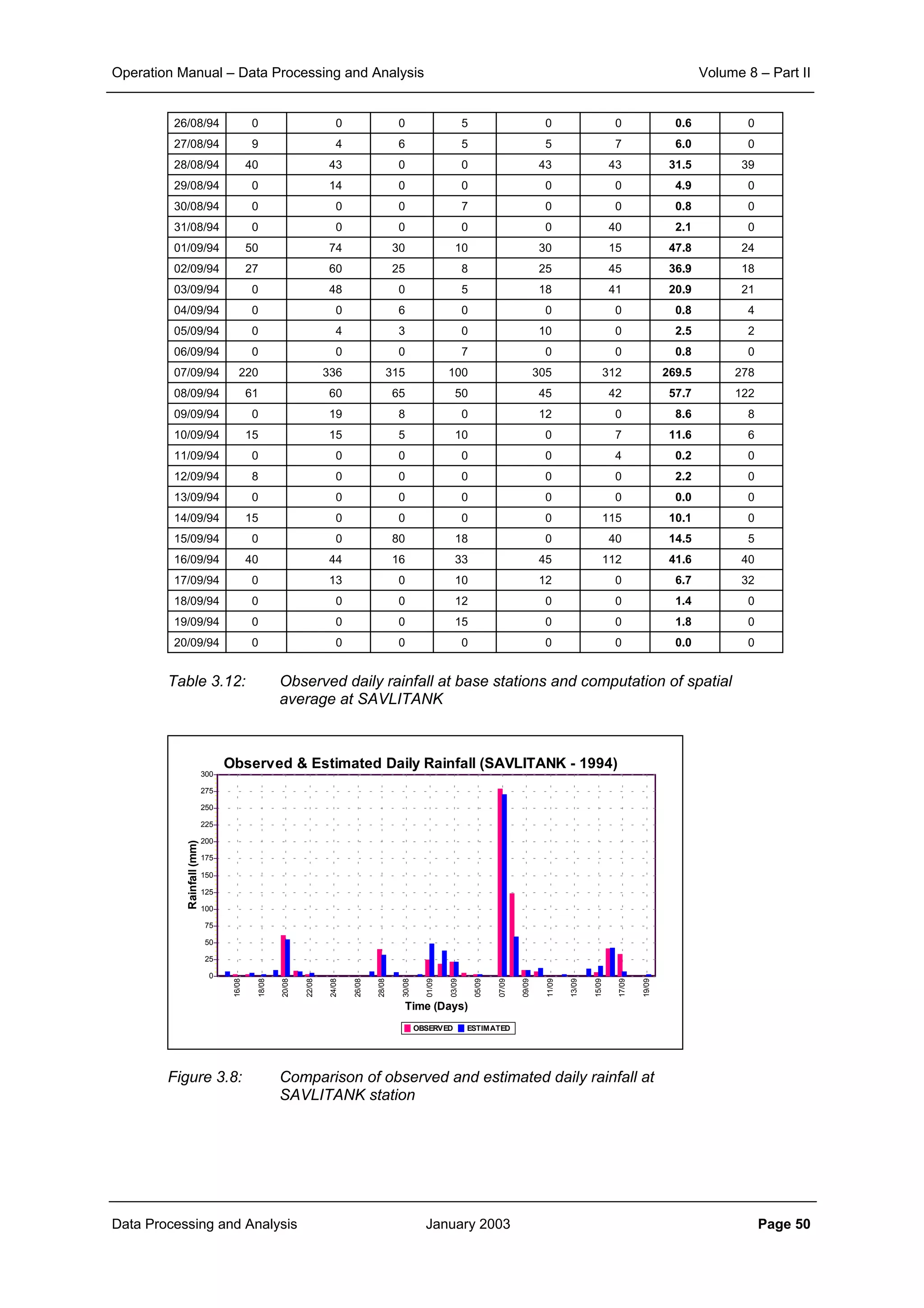
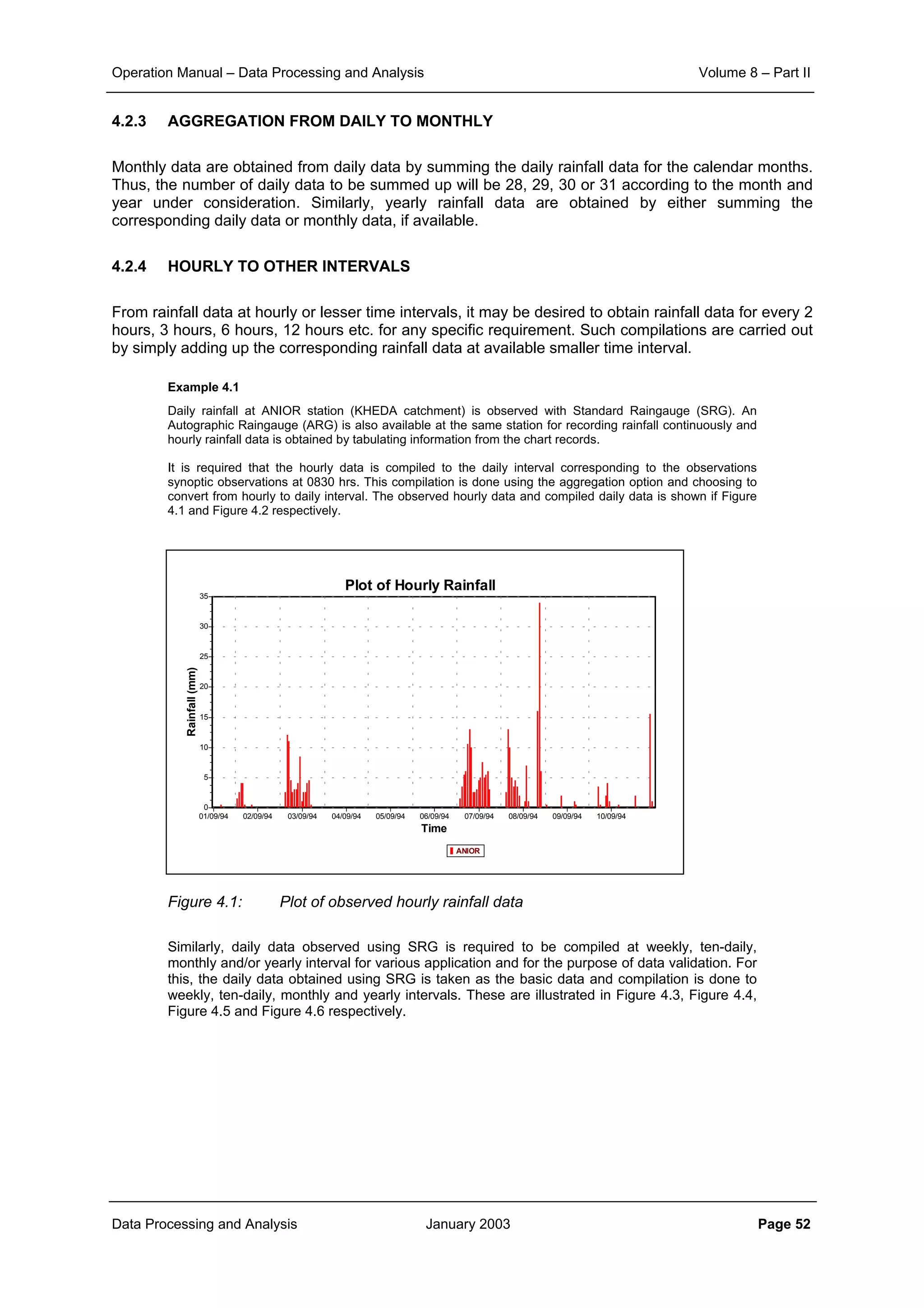
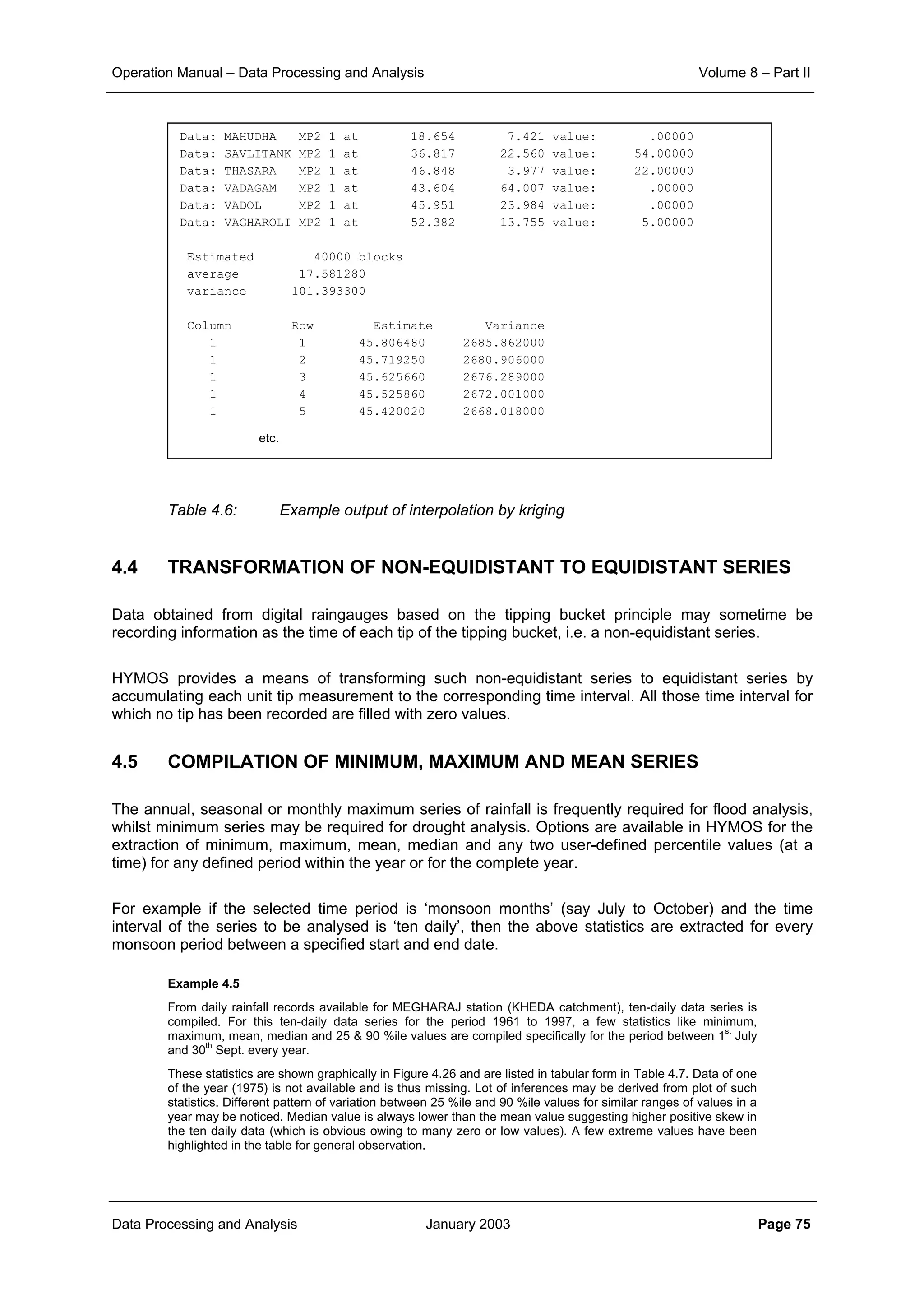
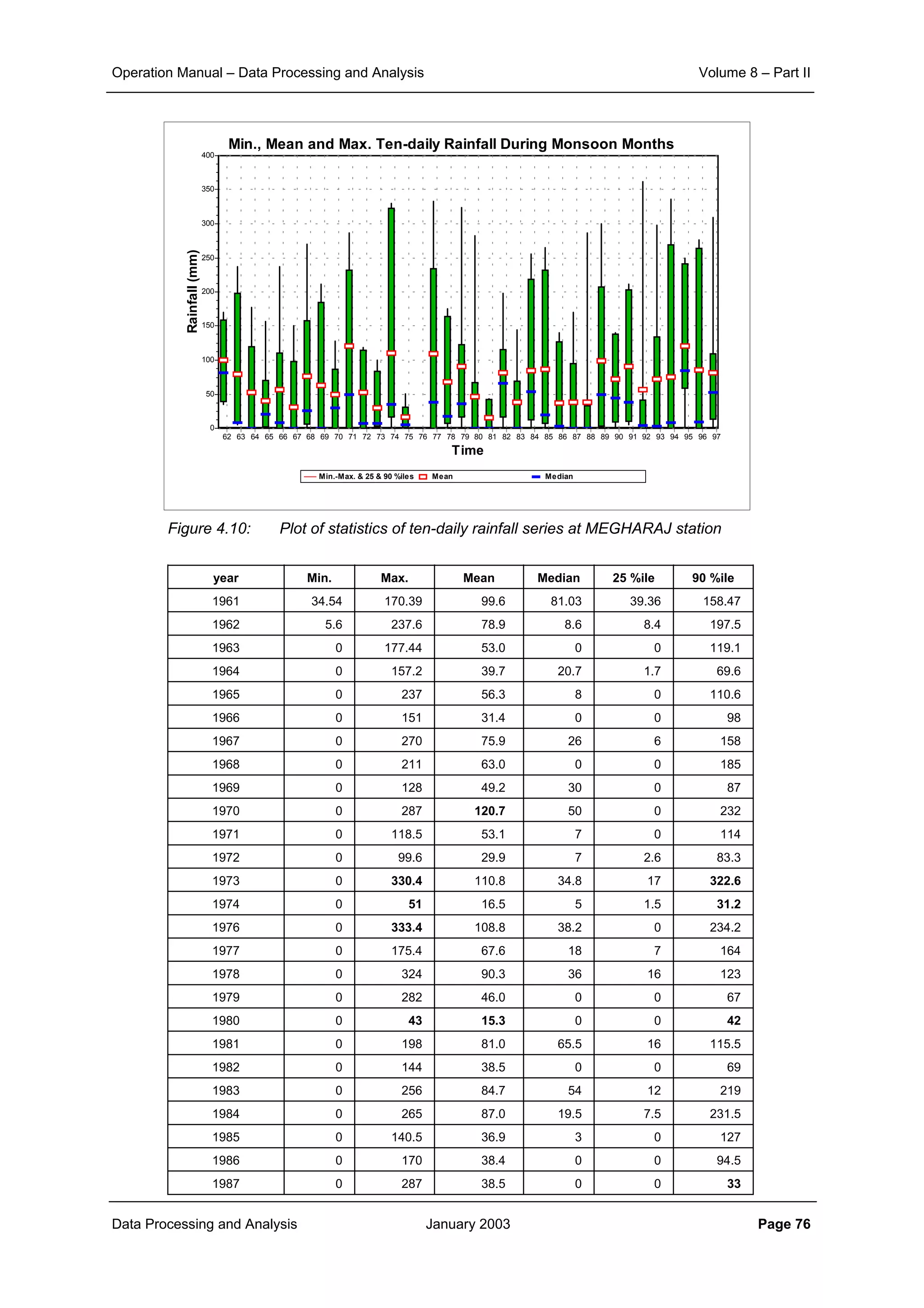
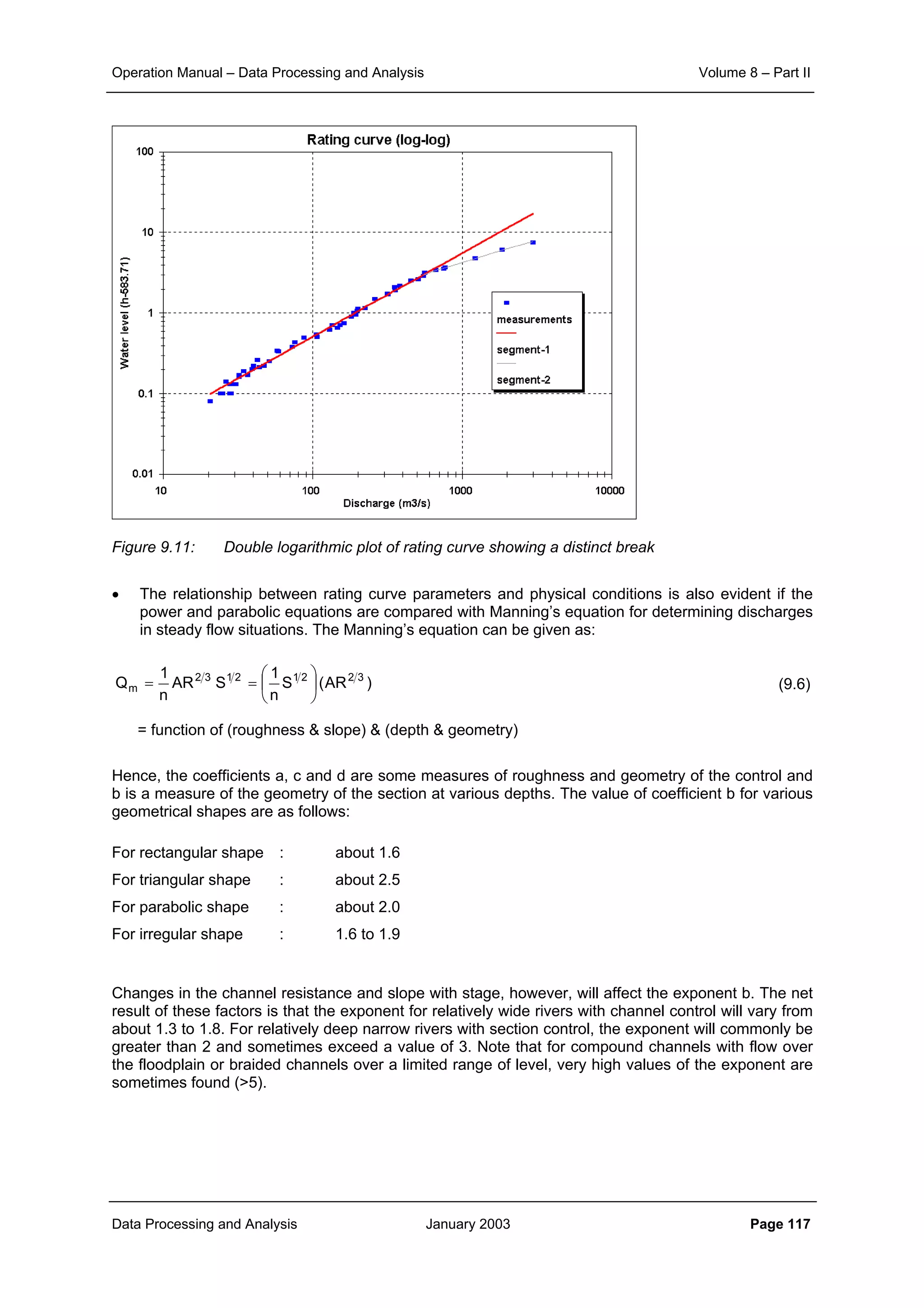
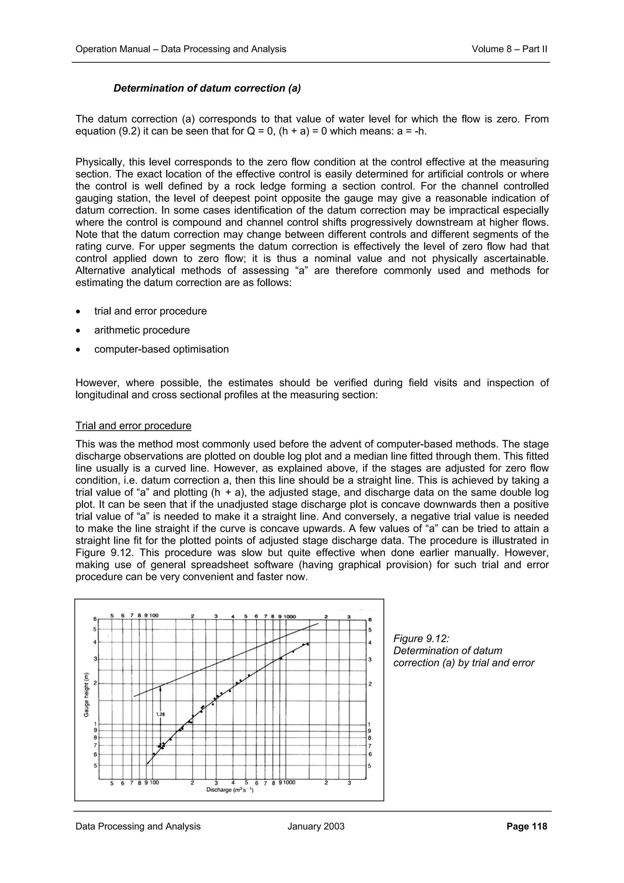
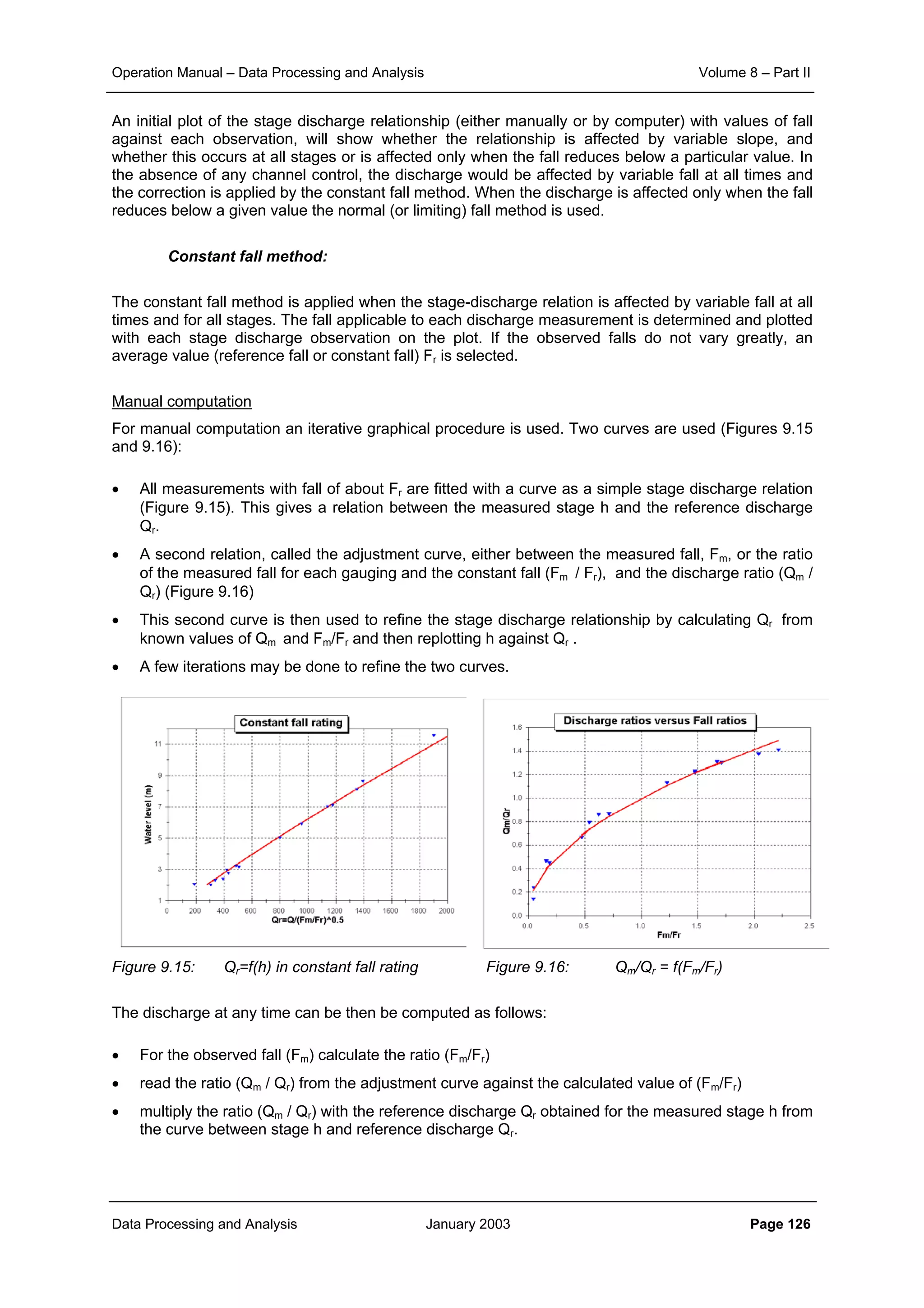
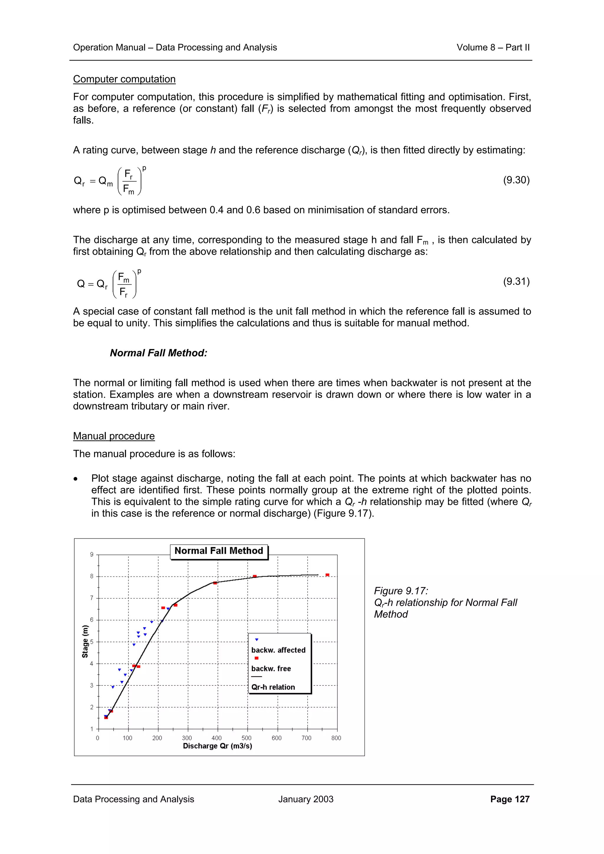
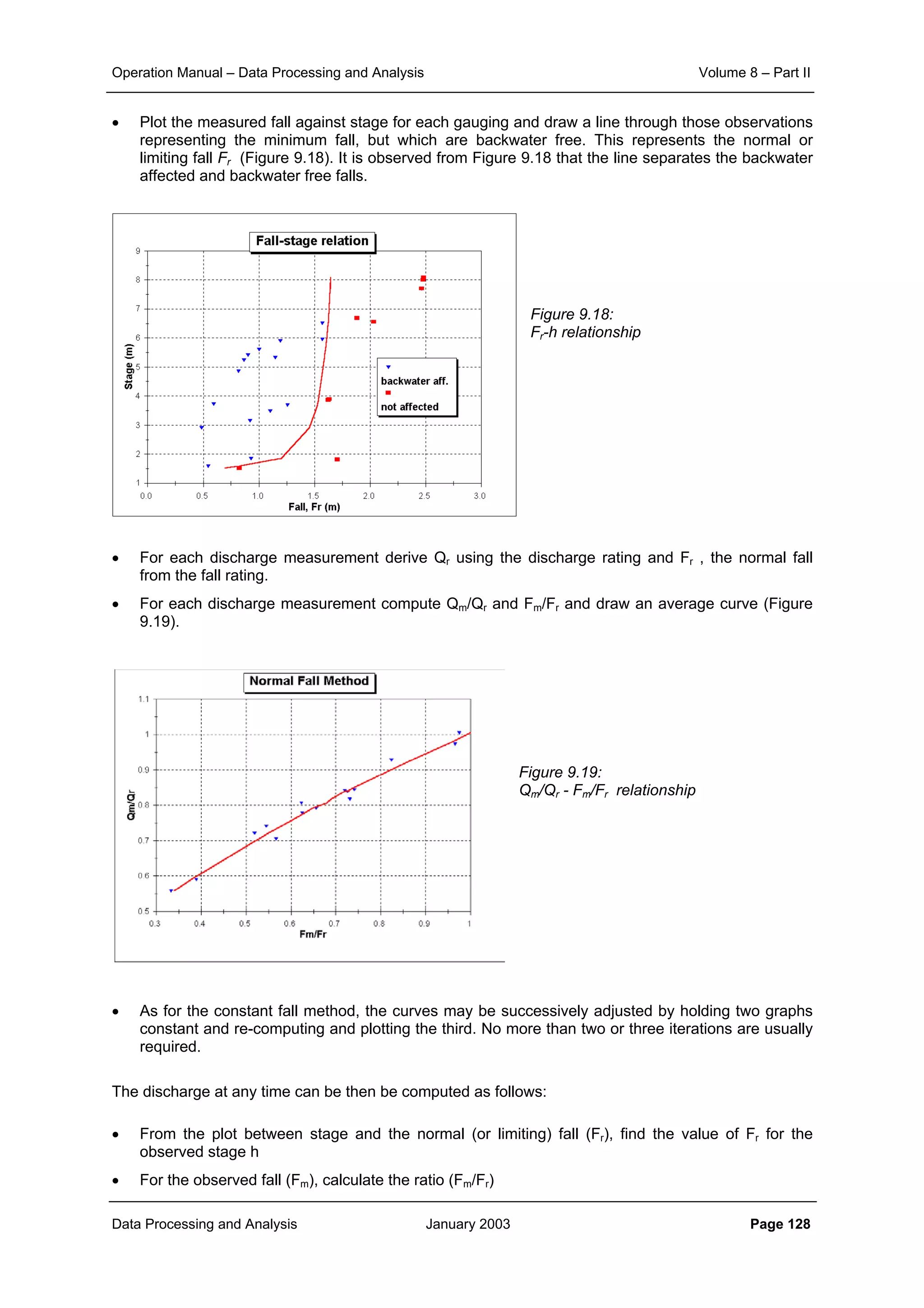
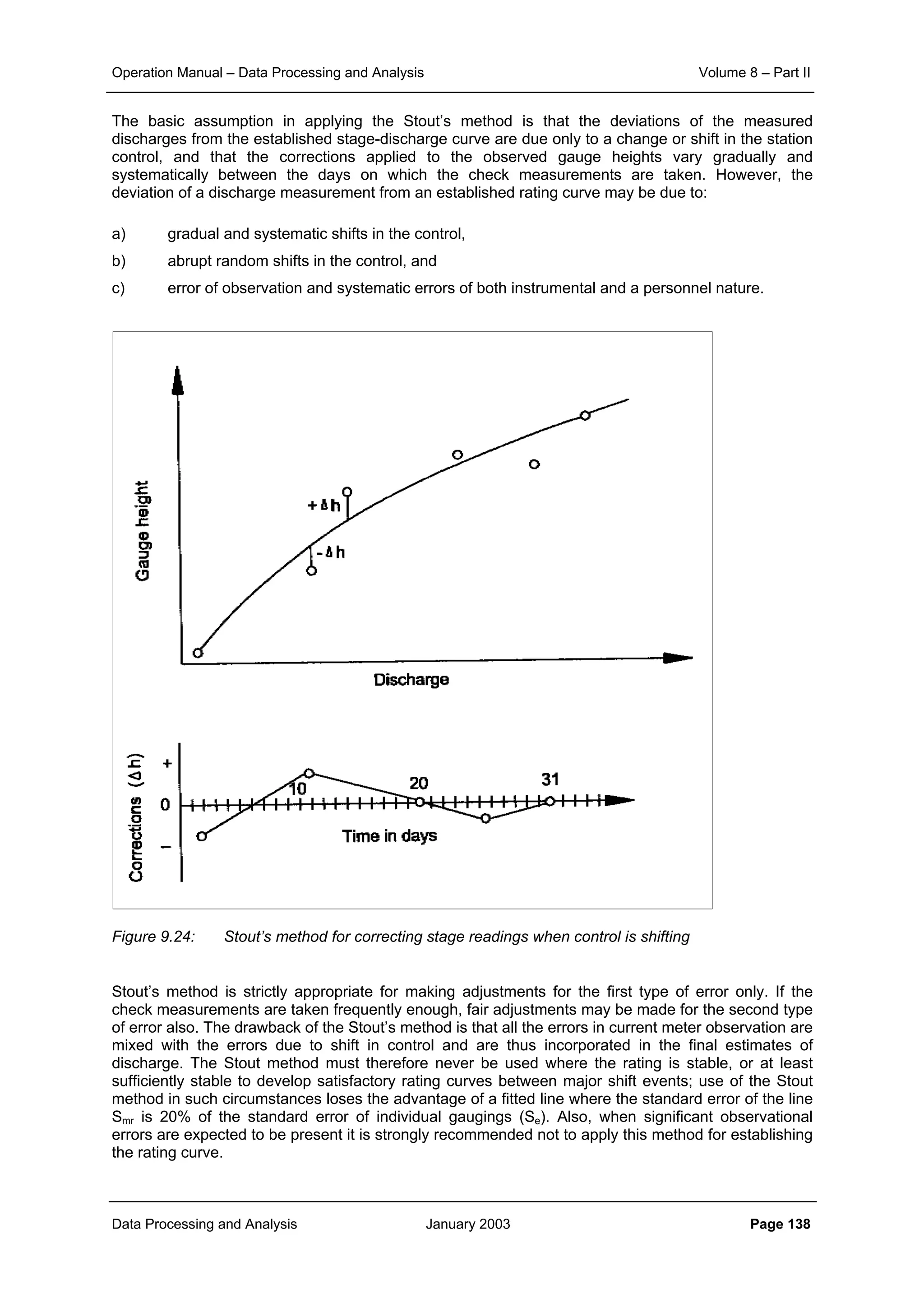
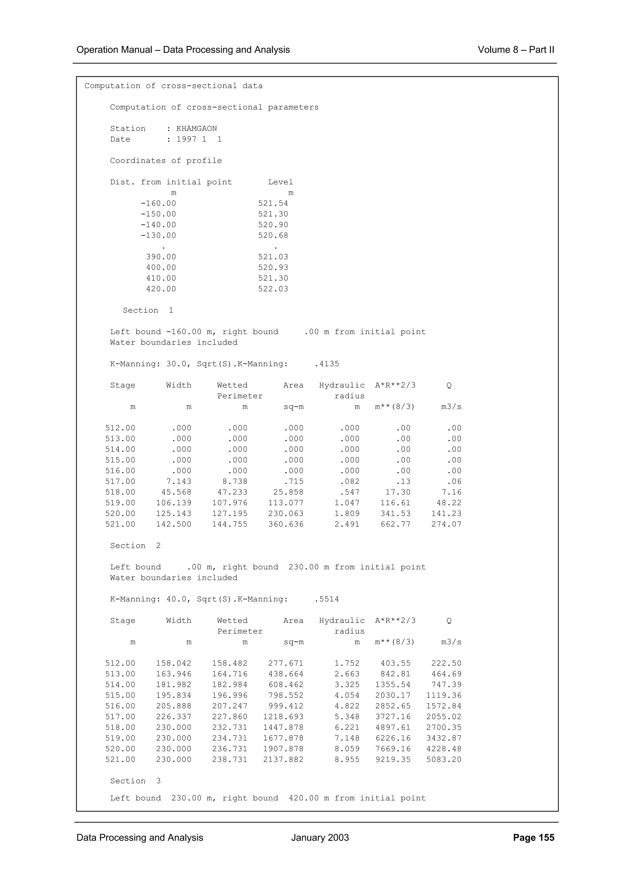
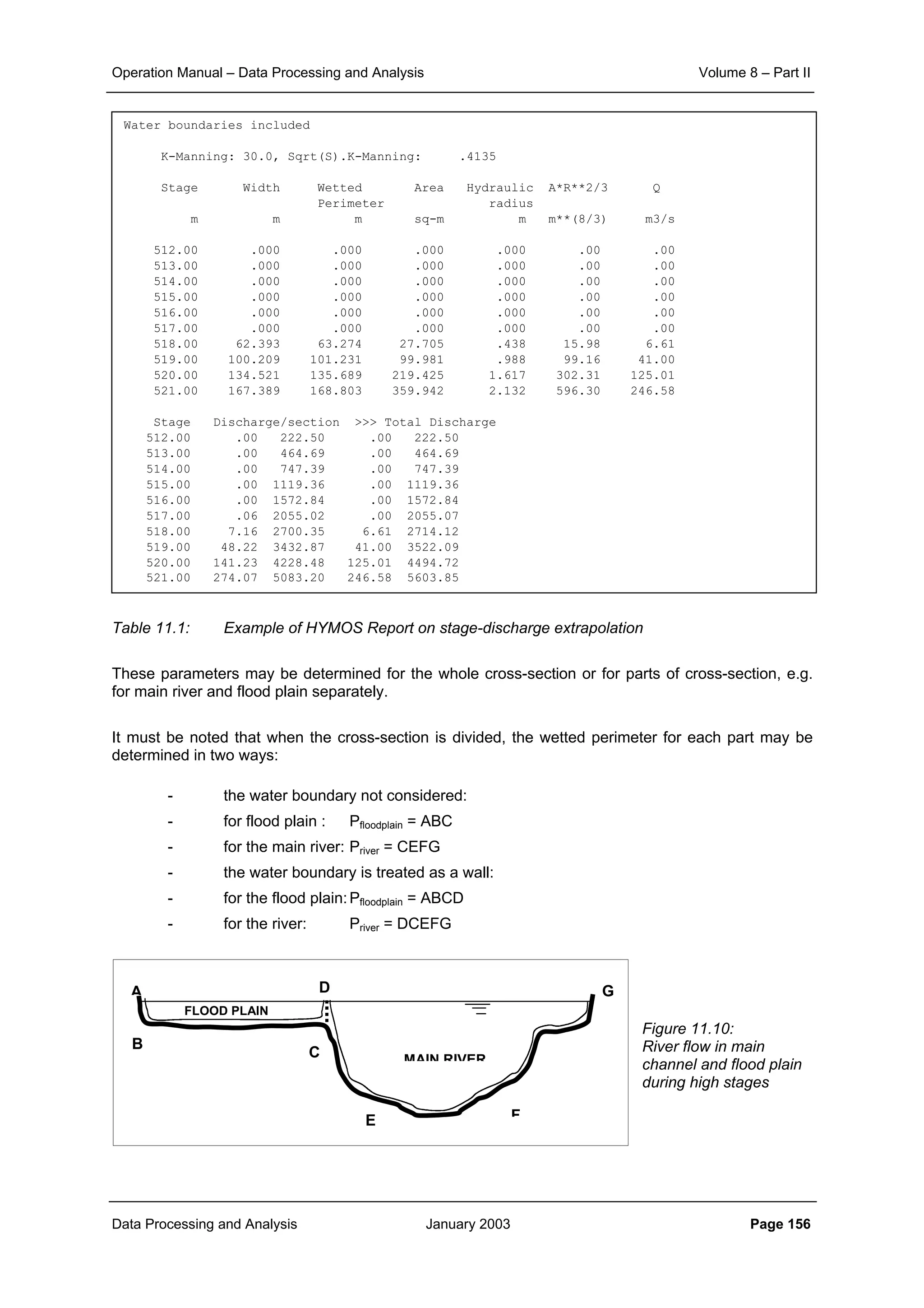
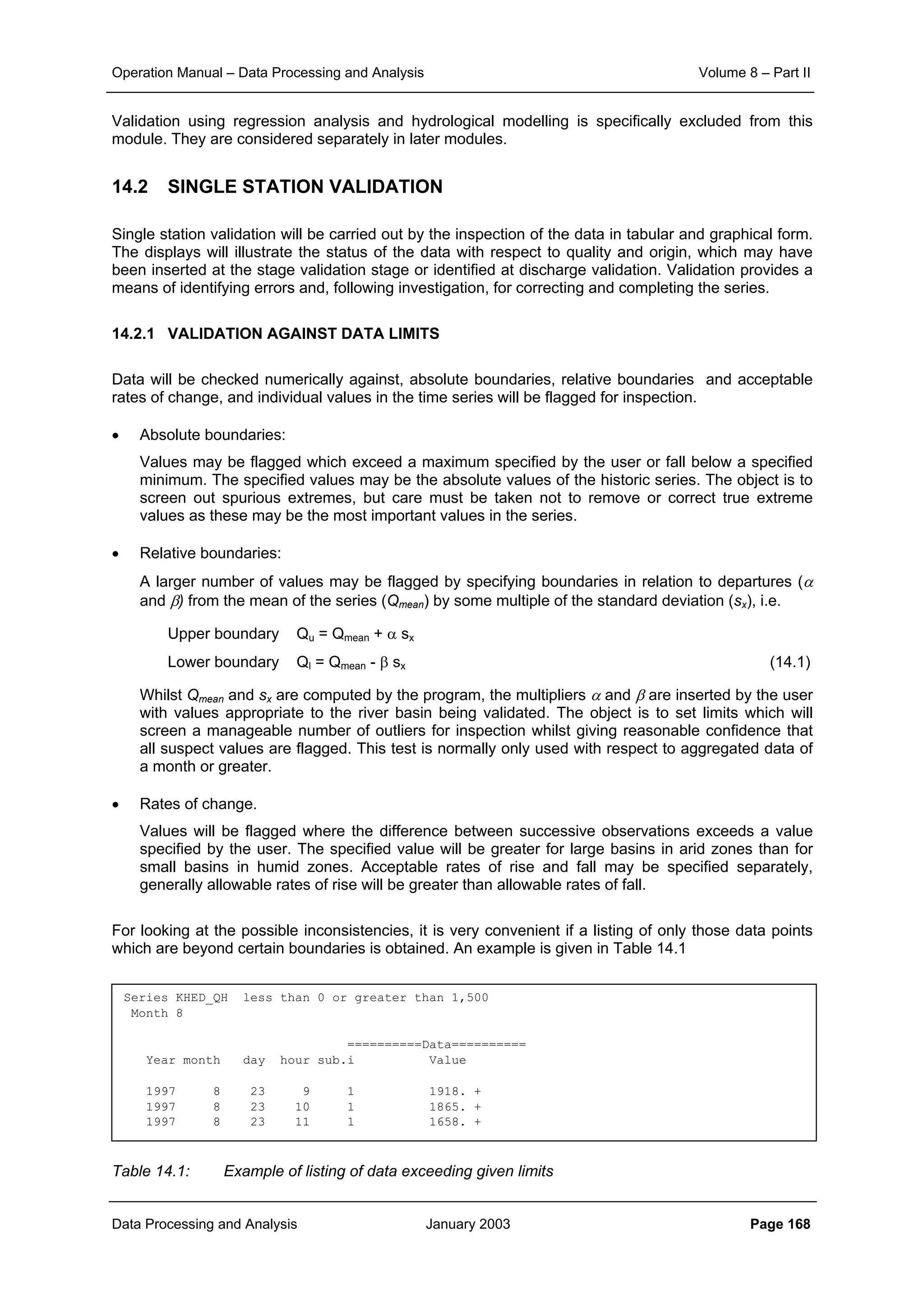
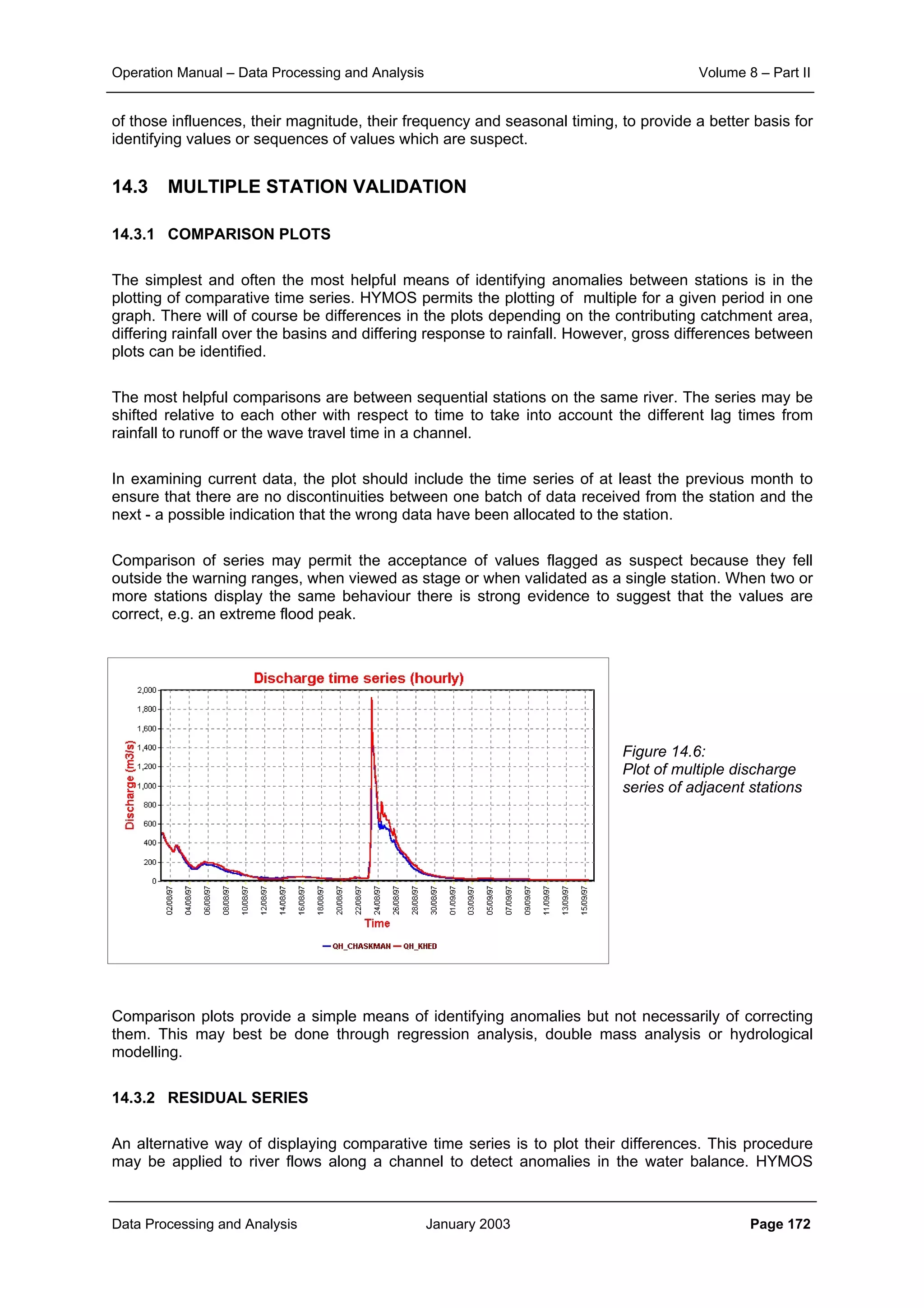
This document provides guidance on secondary validation procedures for hydro-meteorological and surface water quantity and quality data as part of a hydrological information system for 9 states in India. It describes various validation checks that can be performed on rainfall, climatic, water level, discharge, and sediment data including time series analysis, comparison against data limits, double mass curves, and spatial analysis techniques. The document also outlines procedures for correcting and completing data using neighboring station information, interpolation, and rating curves. The overall goal is to ensure standardized and high quality data processing.


![Operation Manual – Data Processing and Analysis Volume 8 – Part II
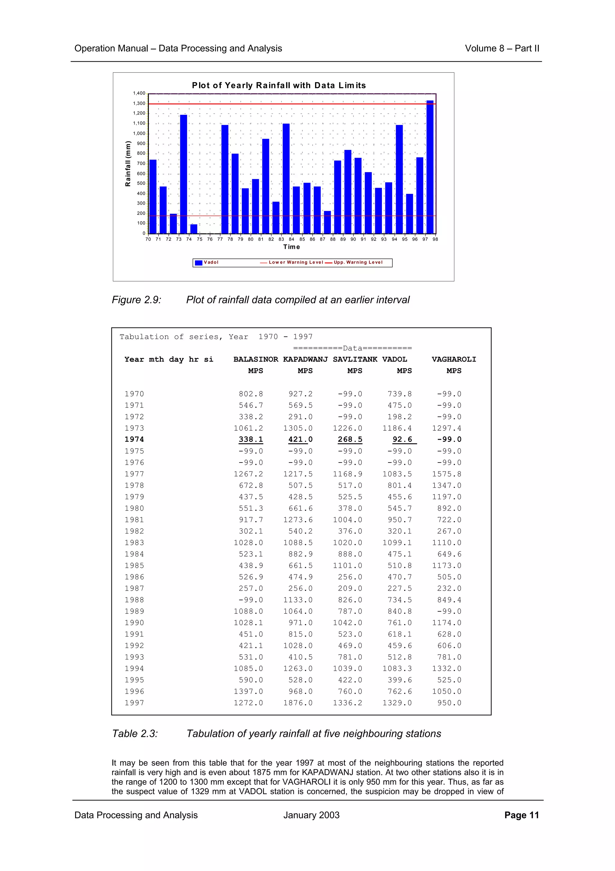
Data Processing and Analysis January 2003 Page 3
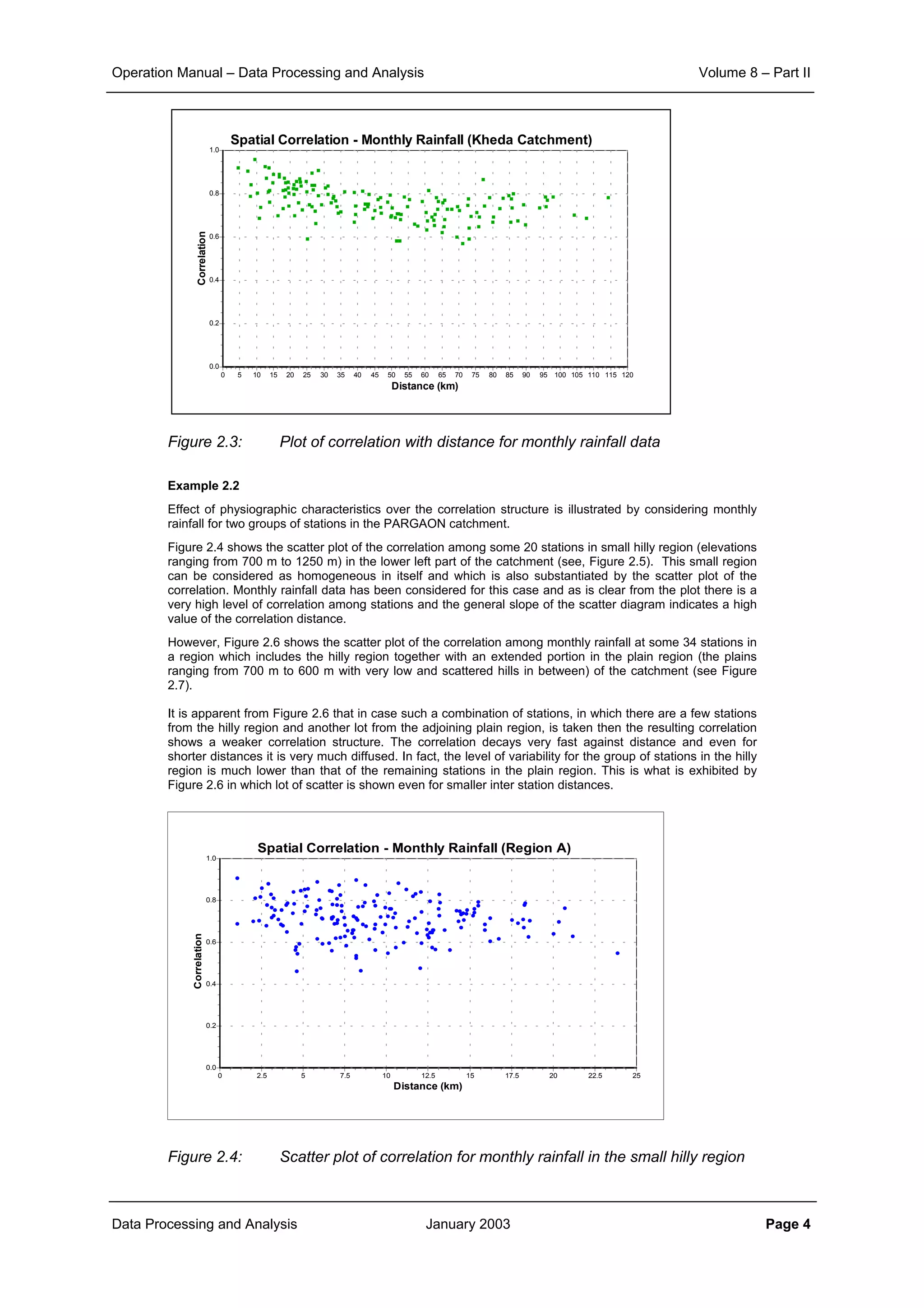
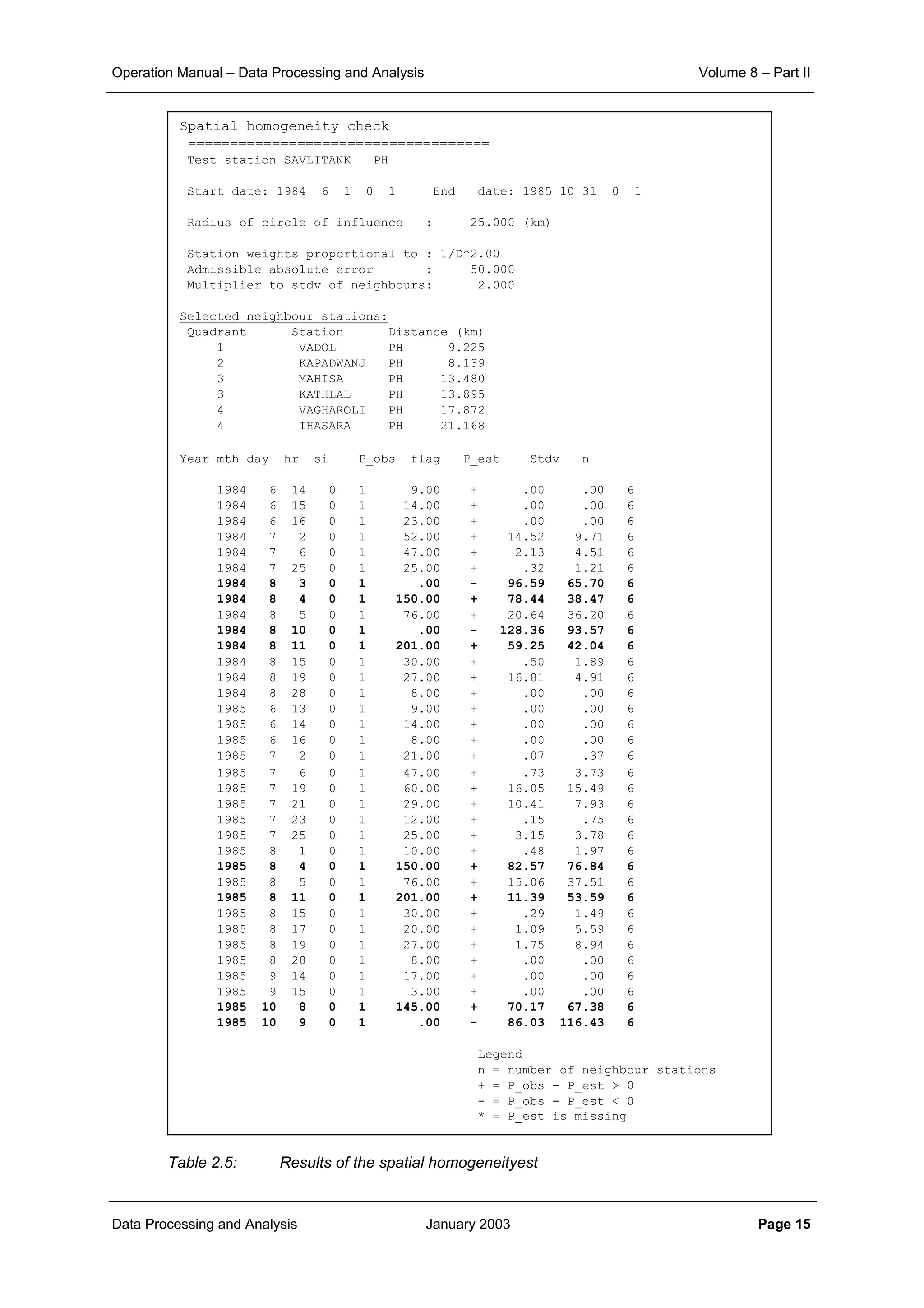
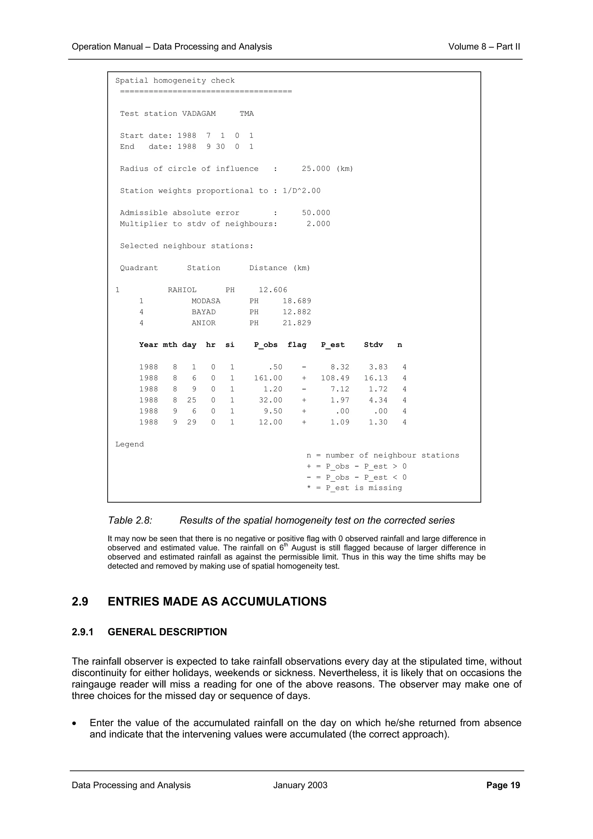
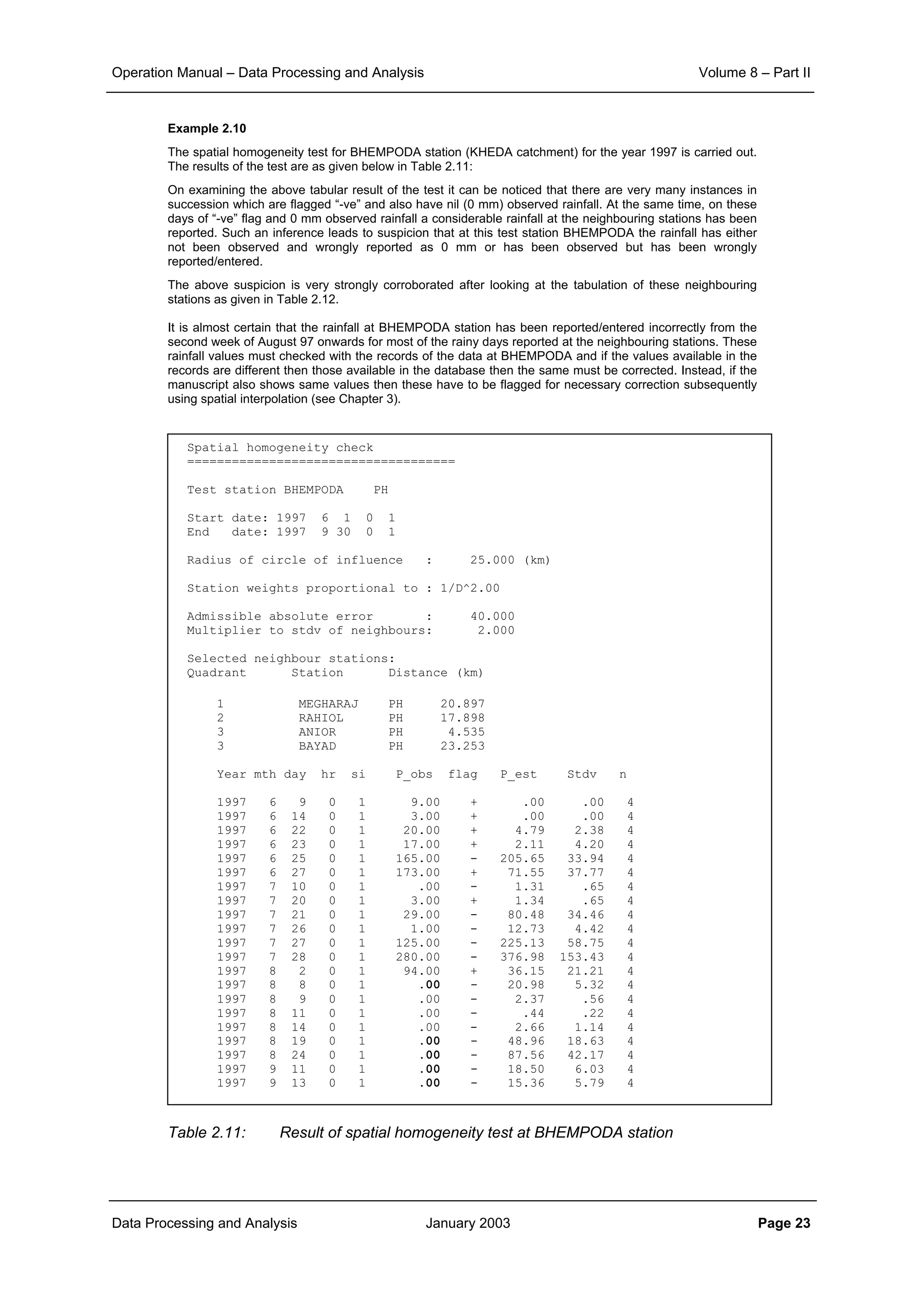
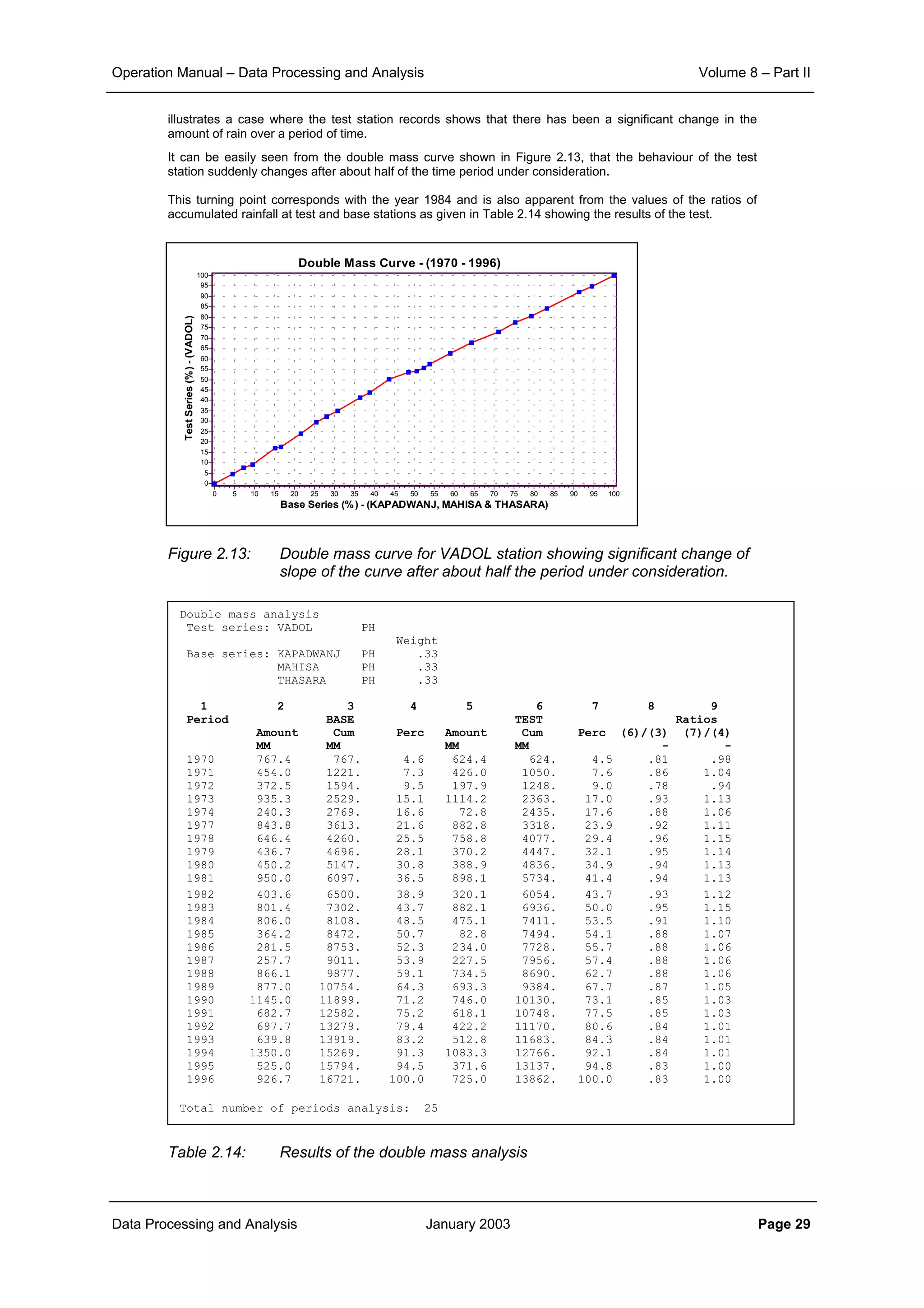
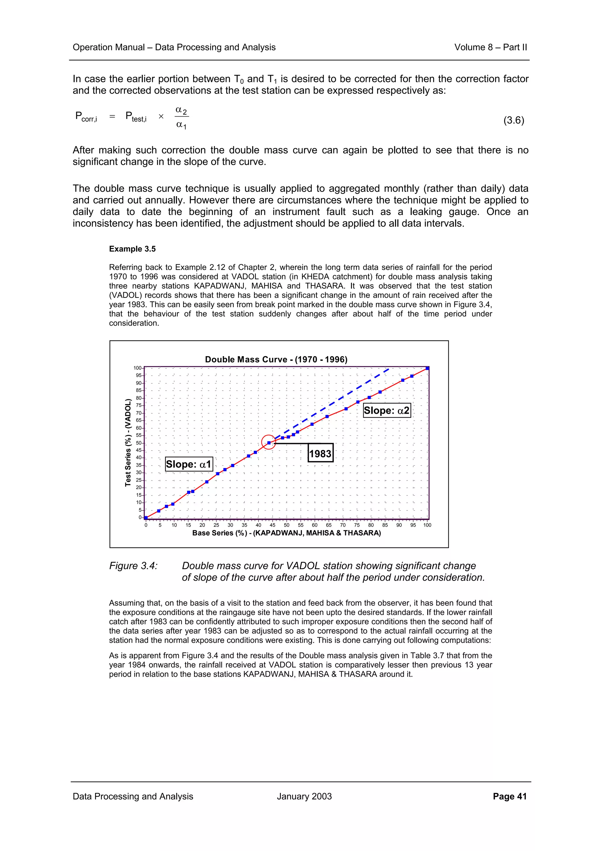
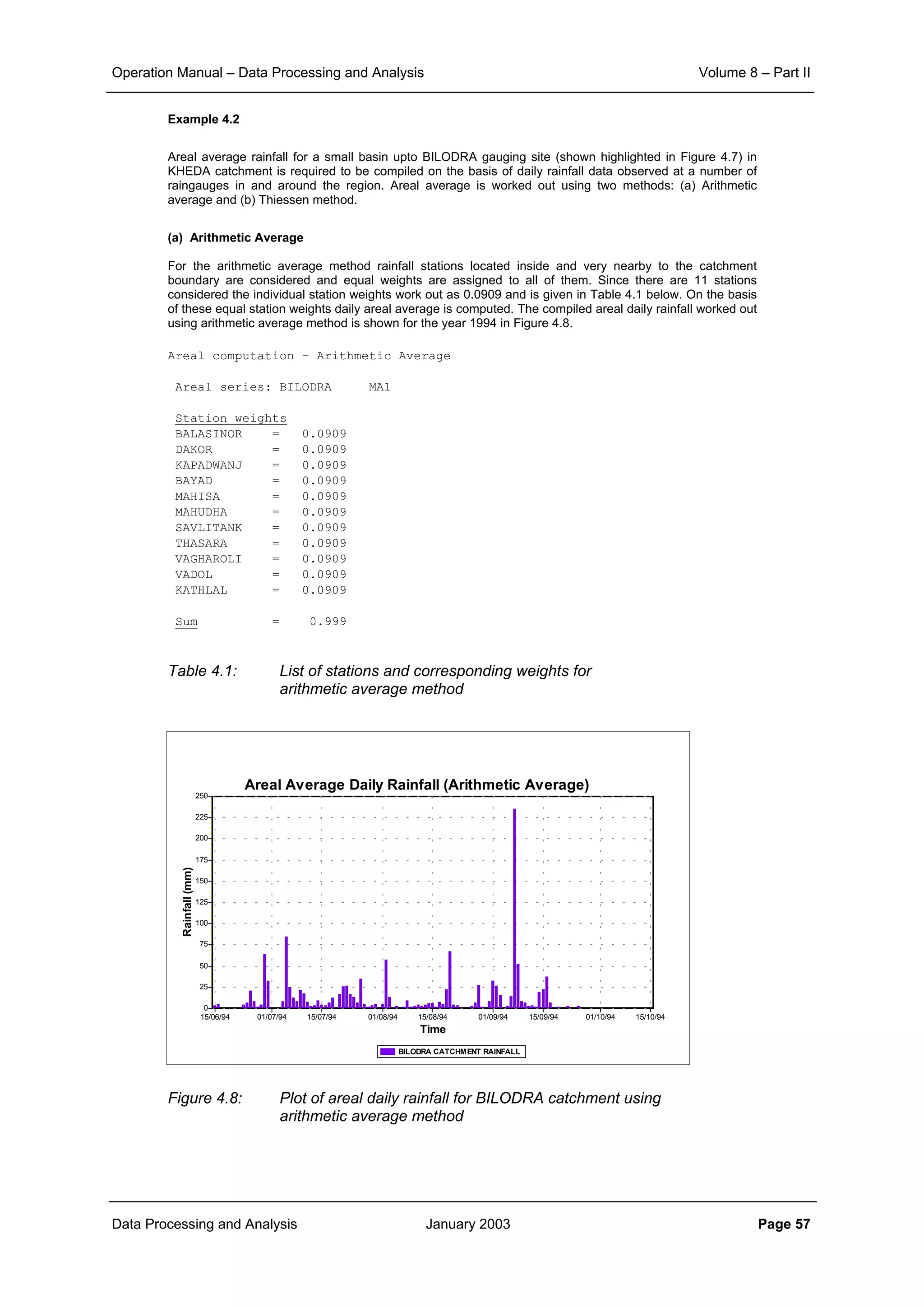
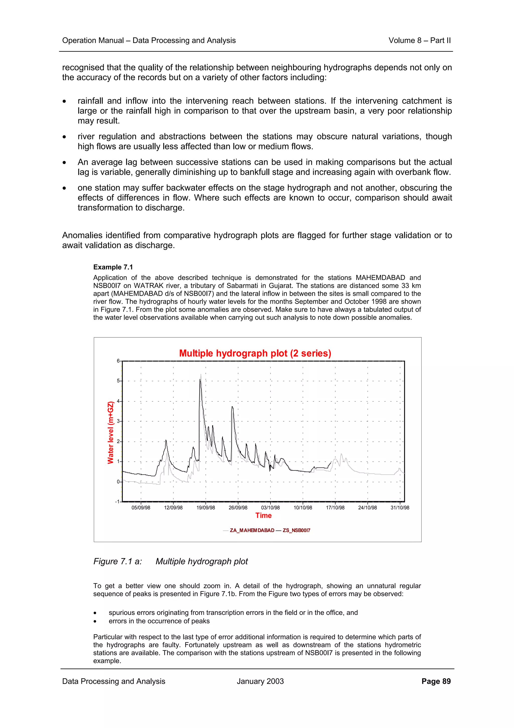
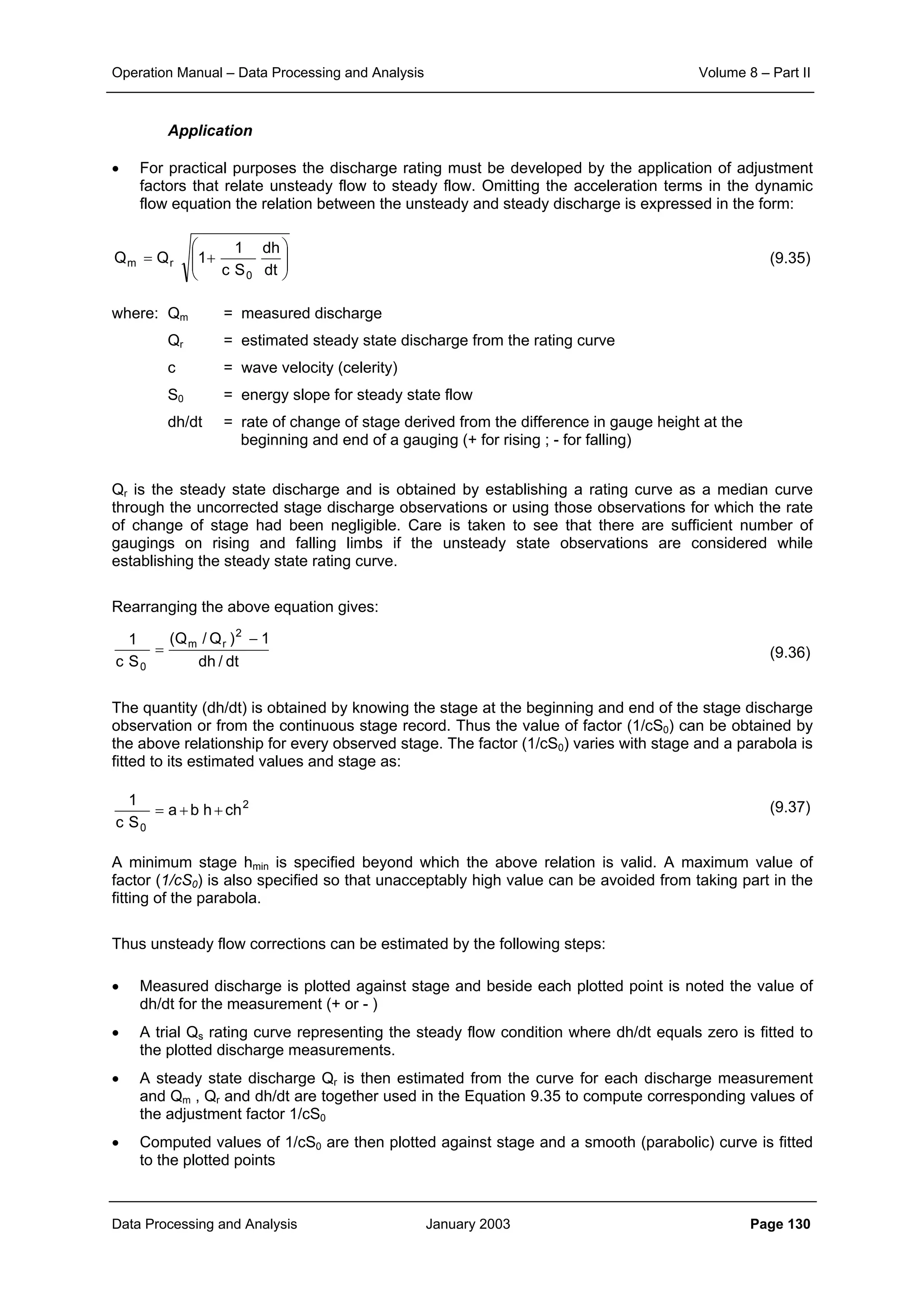
Example 2.1:
The effect of aggregation of data to different time interval and that of the inter-station distances on the
correlation structure is illustrated here.
The scatter plot of correlation between various rainfall stations of the KHEDA catchment for the daily, ten
daily and monthly rainfall data is shown in Figure 2.1, Figure 2.2 and Figure 2.3 respectively.
From the corresponding correlation for same distances in these three figures it can be noticed that
aggregation of data from daily to ten daily and further to monthly level increases the level of correlation
significantly. At the same time it can also be seen that the general slope of the scatter points becomes
flatter as the aggregation is done. This demonstrates that the correlation distance for monthly interval is
much more than that for ten daily interval. And similarly the correlation, which sharply reduces with
increase in distance for the case of daily time interval, does maintain its significance over quite longer
distances.
Figure 2.1: Plot of correlation with distance for daily rainfall data
Figure 2.2: Plot of correlation with distance for ten-daily rainfall data
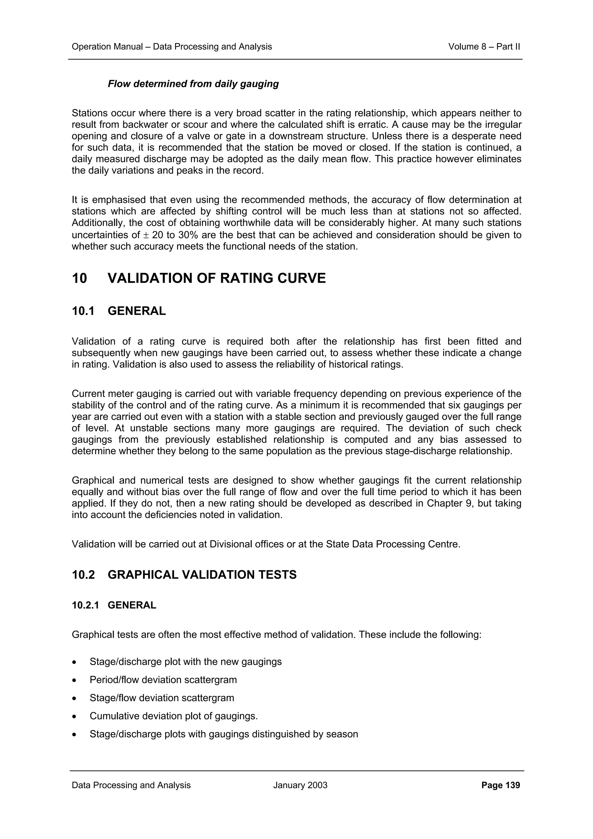
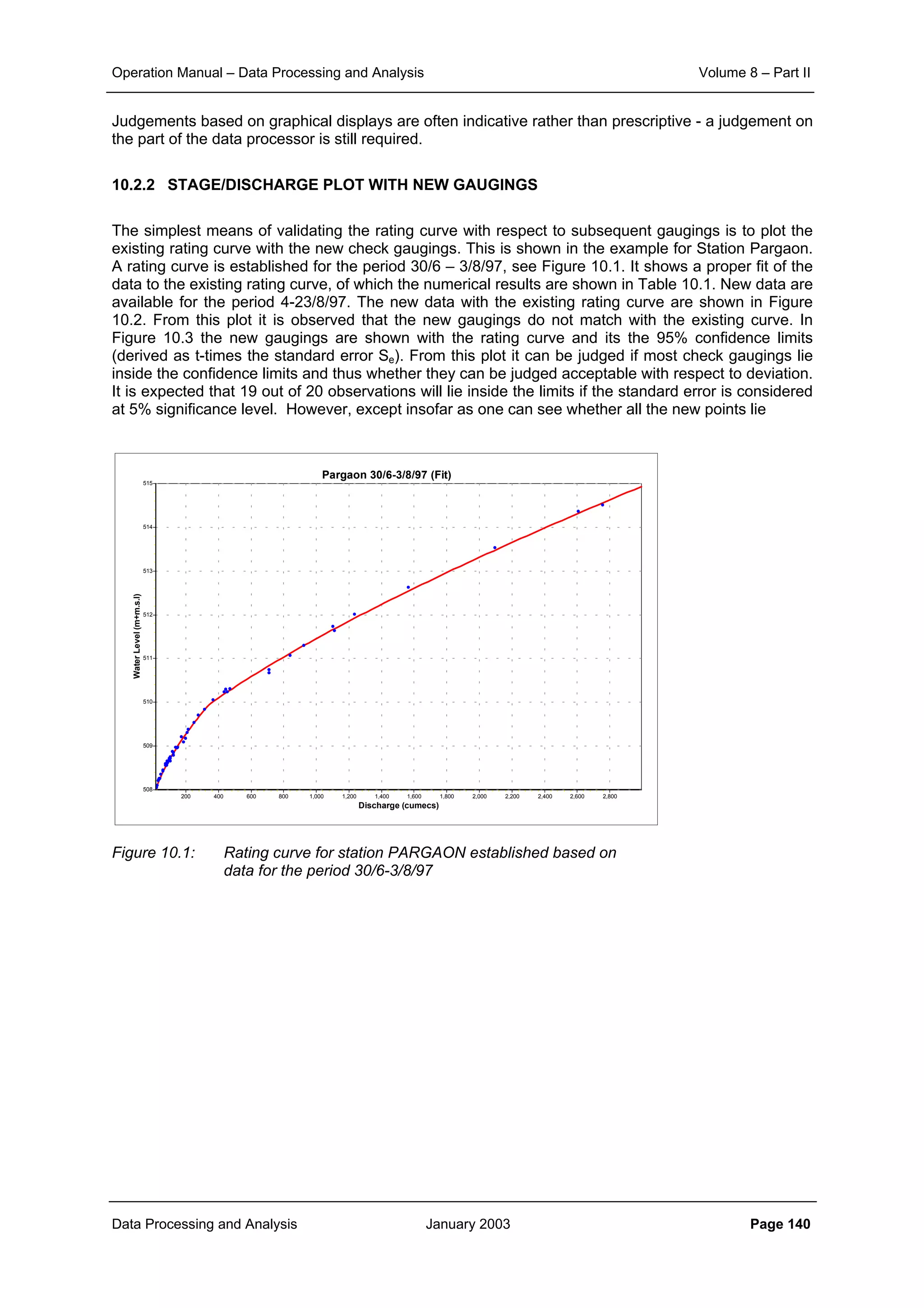
Spatial Correlation - Daily Rainfall (Kheda Catchment)
Distance [km]
120110100908070605040302010
Correlation
1.0
0.8
0.6
0.4
0.2
0.0
Spatial Correlation - 10 Daily Rainfall (Kheda Catchment)
Distance (km)
12011511010510095908580757065605550454035302520151050
Correlation
1.0
0.8
0.6
0.4
0.2
0.0](https://image.slidesharecdn.com/download-manuals-surfacewater-manual-swvolume8operationmanualdataprocessingpartii-140509011631-phpapp01/75/Download-manuals-surface-water-manual-sw-volume8operationmanualdataprocessingpartii-8-2048.jpg)


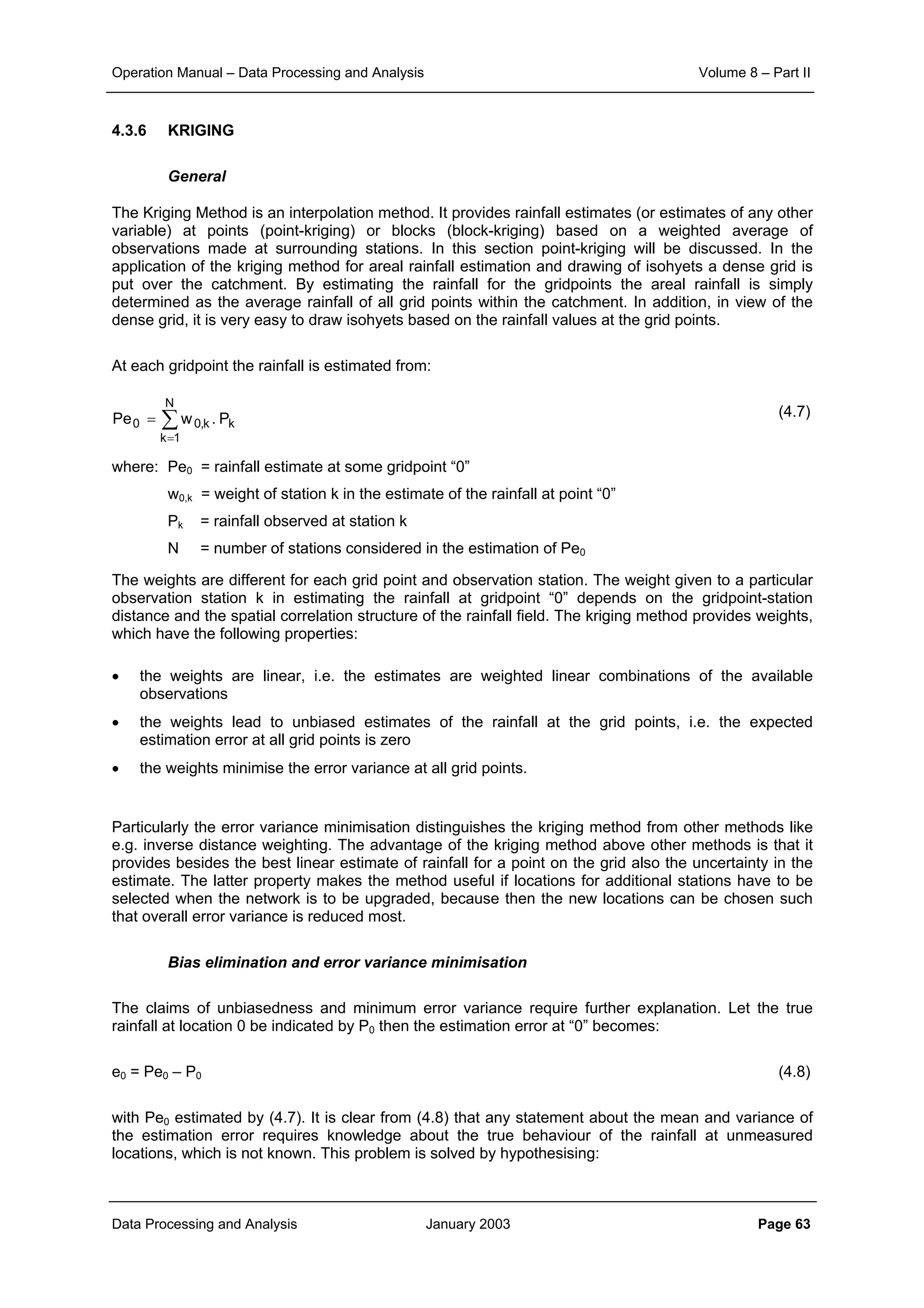
![Operation Manual – Data Processing and Analysis Volume 8 – Part II
Data Processing and Analysis January 2003 Page 64
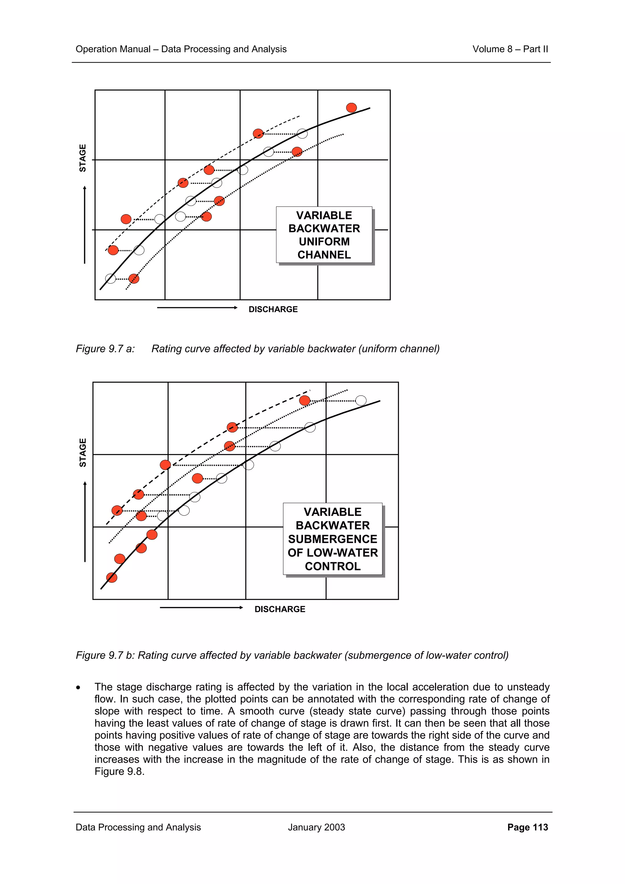
• that the rainfall in the catchment is statistically homogeneous so that the rainfall at all observation
stations is governed by the same probability distribution
• consequently, under the above assumption also the rainfall at the unmeasured locations in the
catchment follows the same probability distribution as applicable to the observation sites.
Hence, any pair of locations within the catchment (measured or unmeasured) has a joint probability
distribution that depends only on the distance between the locations and not on their locations. So:
• at all locations E[P] is the same and hence E[P(x1)] – E[P(x1-d)] = 0, where d refers to distance
• the covariance between any pair of locations is only a function of the distance d between the
locations and not dependent of the location itself: C(d).
The unbiasedness implies:
Hence for each and every gridpoint the sum of the weights should be 1 to ensure unbiasedness:
(4.9)
The error variance can be shown to be (see e.g. Isaaks and Srivastava, 1989):
(4.10)
where 0 refers to the site with unknown rainfall and i,j to the observation station locations. Minimising
the error variance implies equating the N first partial derivatives of σe
2
to zero to solve the w0,i. In
doing so the weights w0,i will not necessarily sum up to 1 as it should to ensure unbiasedness.
Therefore, in the computational process one more equation is added to the set of equations to solve
w0,i, which includes a Lagrangian multiplyer µ. The set of equations to solve the stations weights, also
called ordinary kriging system, then reads:
C . w = D (4.11)
where:
Note that the last column and row in C are added because of the introduction of the Lagrangian
multiplyer µ in the set of N+1 equations. By inverting the covariance matrix the station weights to
estimate the rainfall at location 0 follow from (4.11) as:
w = C-1
. D (4.12)
01w]P[E:or0]P[E]P.w[E:so0]e[E
N
1k
k,000
N
1k
kk,00 =
∑ −=−∑=
==
∑∑ ∑
= = =
−+σ=−=σ
N
1i
N
1j
N
1i
i,0i,0j,ij,0i,0
2
P
2
00
2
e Cw2Cww])PPe[(E
=
µ
=
=
1
C
.
.
C
w
.
.
w
01...................1
1C...............C
...
...
1C...............C
N,0
1,0
N,0
1,0
NN1N
N111
DwC
1w
N
1k
k,0 =∑
=](https://image.slidesharecdn.com/download-manuals-surfacewater-manual-swvolume8operationmanualdataprocessingpartii-140509011631-phpapp01/75/Download-manuals-surface-water-manual-sw-volume8operationmanualdataprocessingpartii-69-2048.jpg)
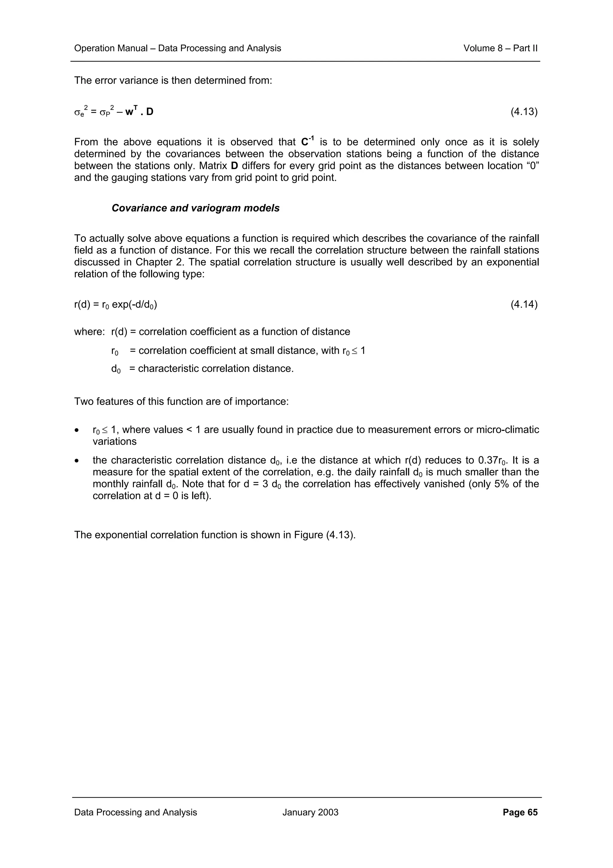
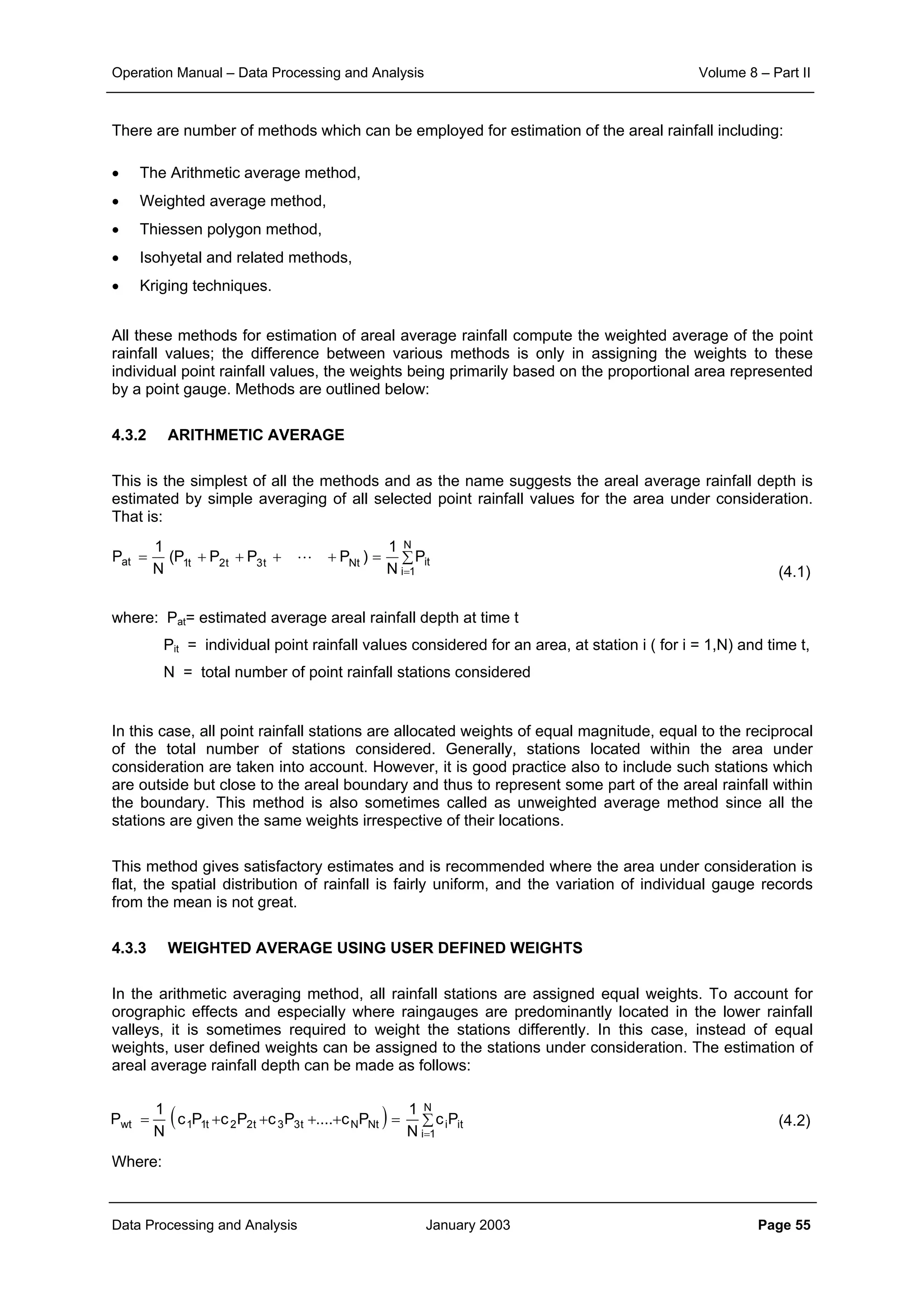
![Operation Manual – Data Processing and Analysis Volume 8 – Part II
Data Processing and Analysis January 2003 Page 66
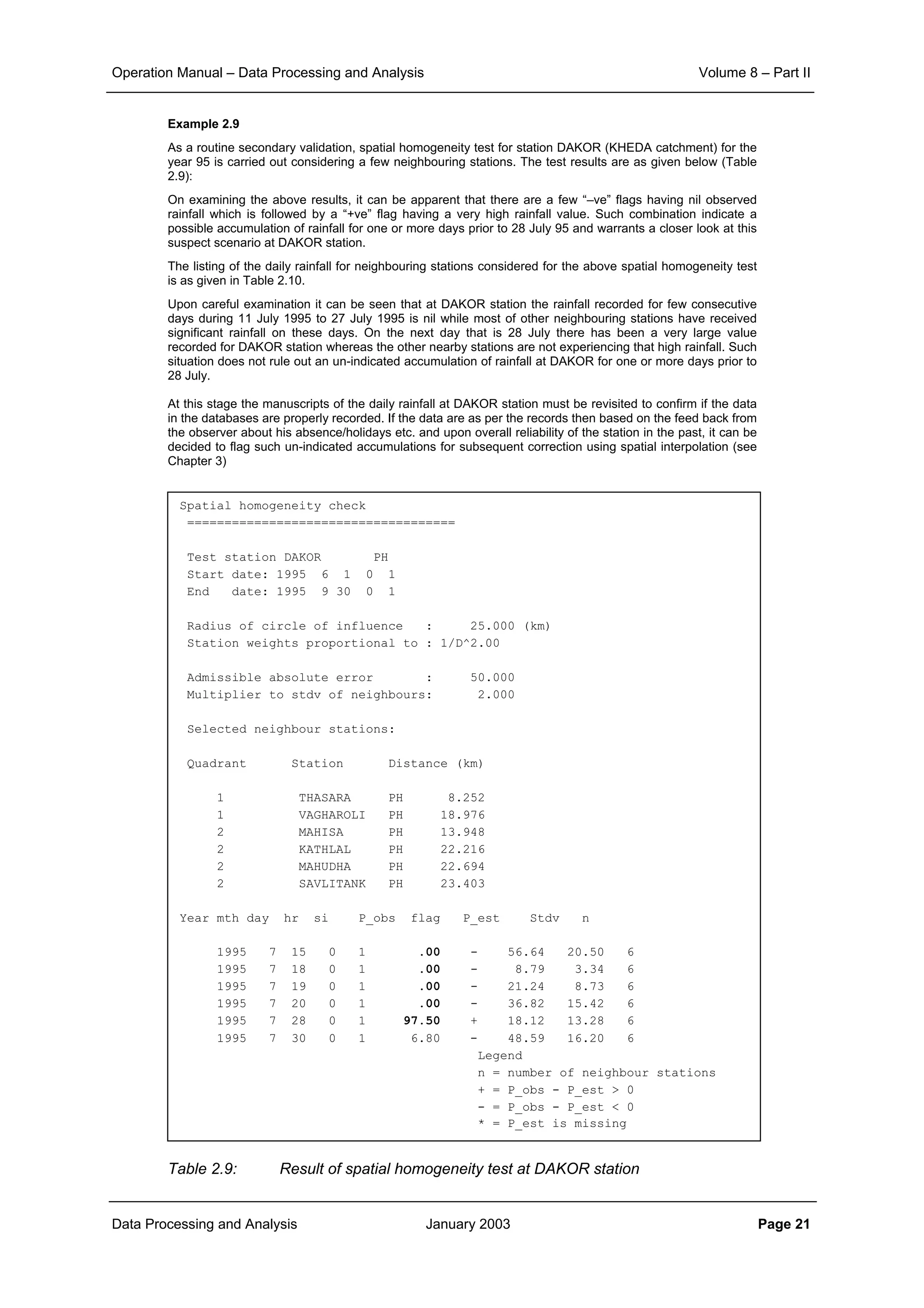
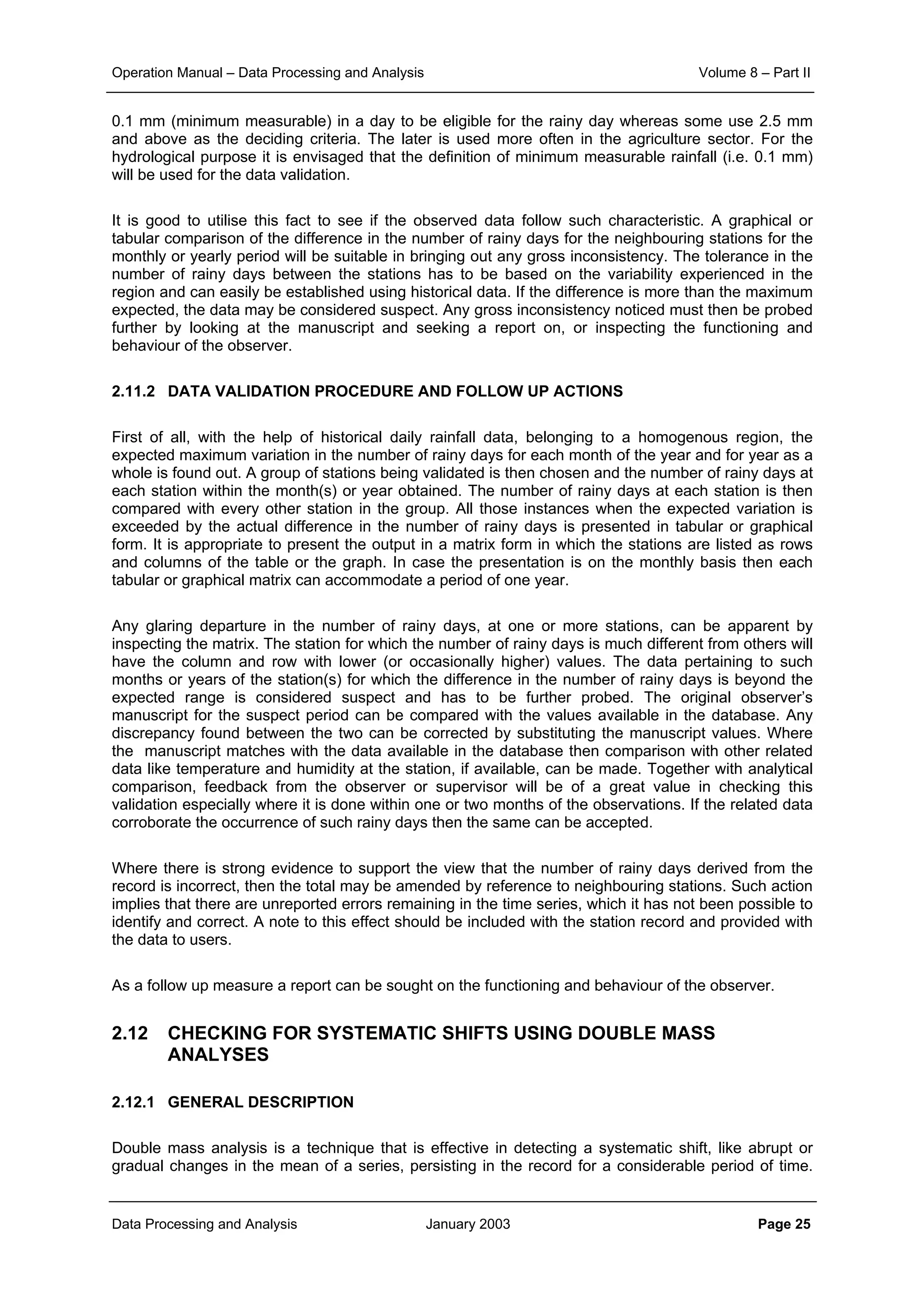
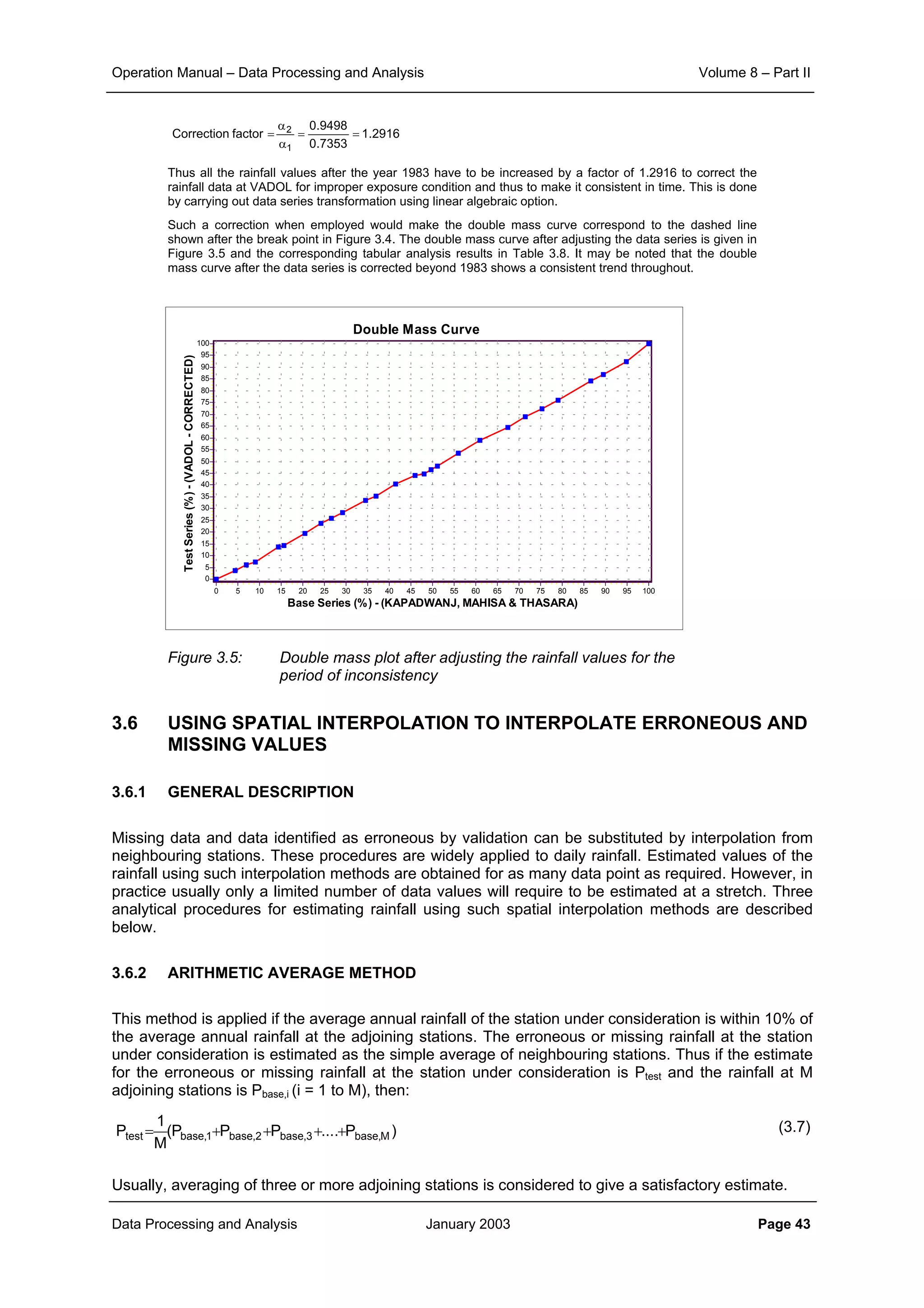
Figure 4.13:
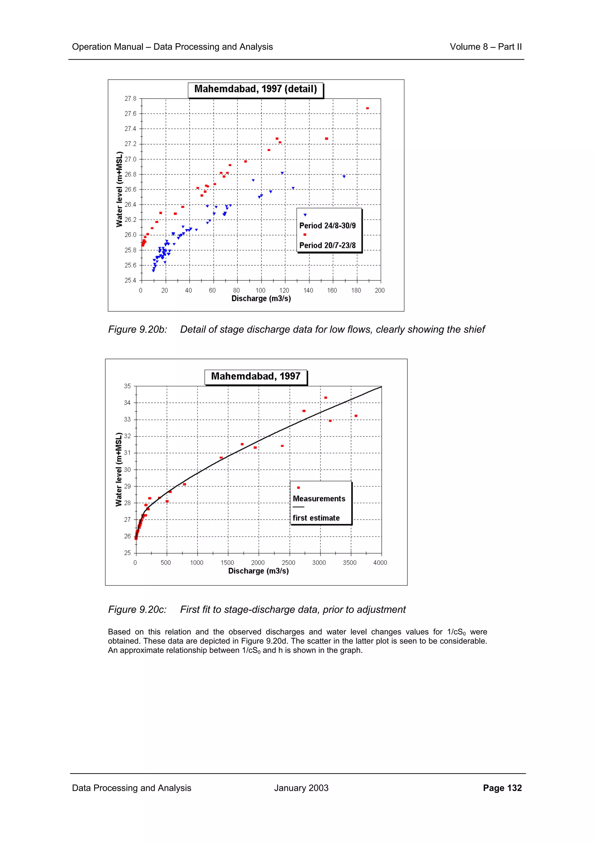
Spatial correlation
structure of rainfall field
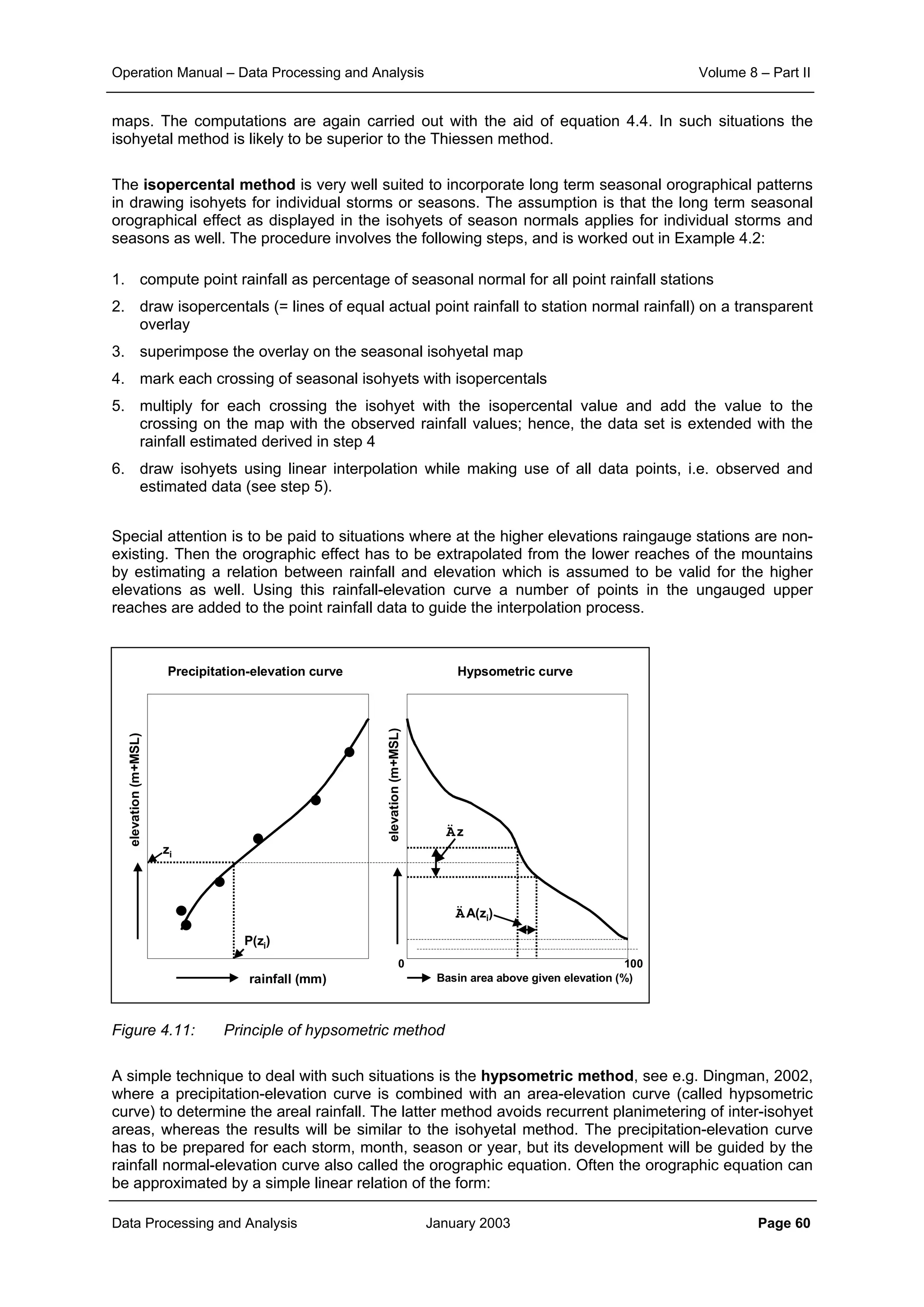
The covariance function of the exponential model is generally expressed as:
(4.15)
Since according to the definition C(d) = r(d)σP
2
, the coefficients C0 and C1 in (4.15) can be related to
those of the exponential correlation model in (4.14) as follows:
C0 = σP
2
(1-r0) ; C1 = σP
2
r0 and a = 3d0 (4.16)
In kriging literature instead of using the covariance function C(d) often the semi-variogram γ(d) is
used, which is halve of the expected squared difference between the rainfall at locations distanced d
apart; γ(d) is easily shown to be related to C(d) as:
γ(d) = ½ E[{P(x1) – P(x1-d)}2
] = σP
2
– C(d) (4.17)
Hence the (semi-)variogram of the exponential model reads:
(4.18)
The exponential covariance and variogram models are shown in Figures 4.14 and 4.15.
0dfor)
a
d3
exp(C)d(C
0dforCC)d(C
1
10
>−=
=+=
0d:for)
a
d3
exp(1CC)d(
0d:for0)d(
10 >
−−+=γ
==γ
1
r0
Distance d
Exponential spatial correlation function
Exponential spatial correlation
function:
r(d) = r0 exp(- d / d0)
0
0.37r0
d0](https://image.slidesharecdn.com/download-manuals-surfacewater-manual-swvolume8operationmanualdataprocessingpartii-140509011631-phpapp01/75/Download-manuals-surface-water-manual-sw-volume8operationmanualdataprocessingpartii-71-2048.jpg)
![Operation Manual – Data Processing and Analysis Volume 8 – Part II
Data Processing and Analysis January 2003 Page 72
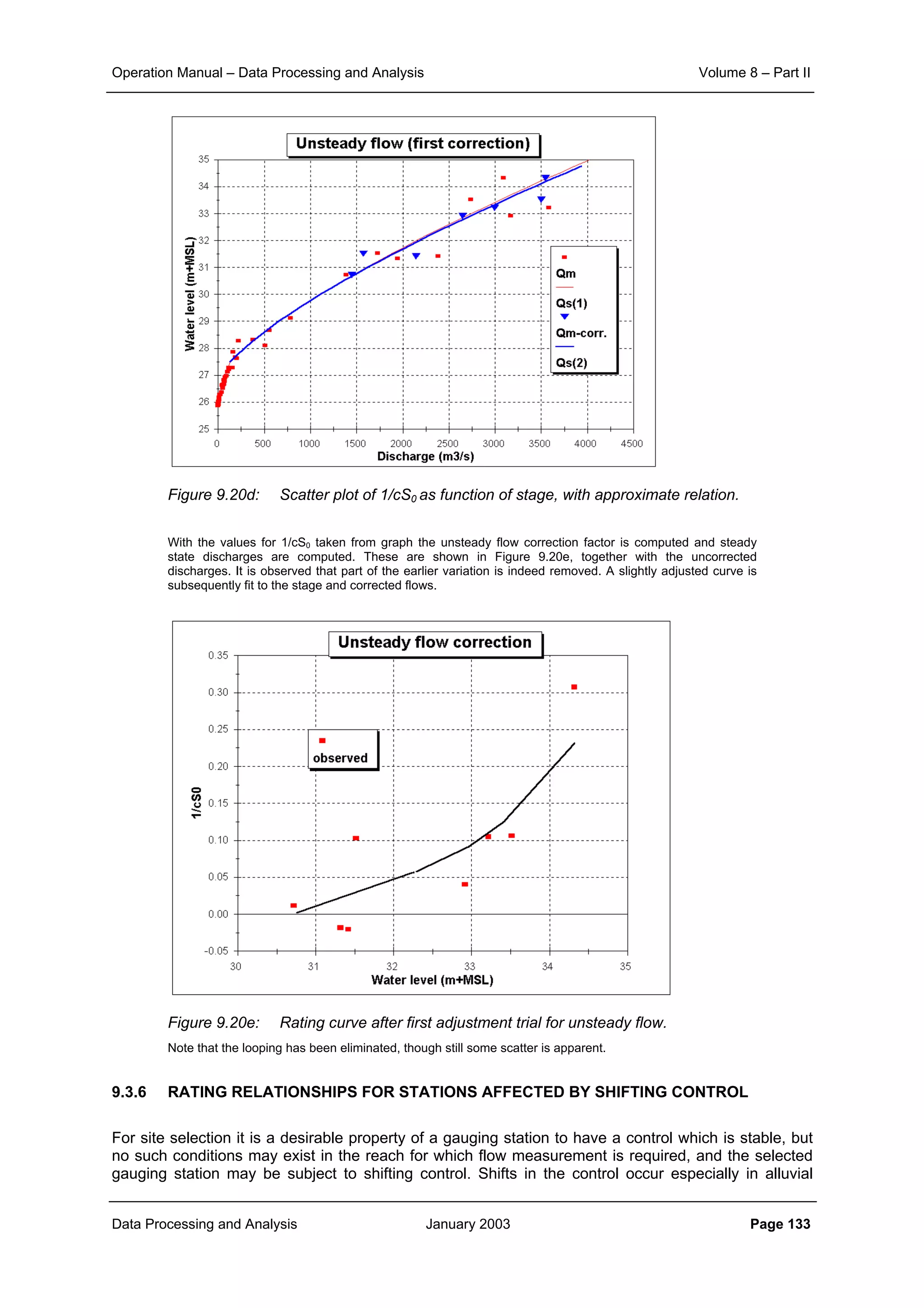
Figure 4.20: Spatial correlation structure of monthly rainfall data in and around
Bilodra catchment (values > 10 mm)
From Figure 4.20 it is observed that the correlation only slowly decays. Fitting an exponential correlation
model to the monthly data gives: r0 ≈ 0.8 and d0 = 410 km. The average variance of the monthly point
rainfall data (>10 mm) amounts approx. 27,000 mm
2
. It implies that the sill of the semi-variogram will be
27,000 mm
2
and the range is approximately 1200 km (≈ 3 d0). The nugget is theoretically σP
2
(1-r0), but is
practically obtained by fitting the semi-variogram model to the semi-variance versus distance plot. In
making this plot a lag-distance is to be applied, i.e. a distance interval for averaging the semi-variances to
reduce the spread in the plot. In the example a lag-distance of 10 km has been applied. The results of the
fit overall and in detail to a spherical semi-variogram model is shown in Figure 4.21. A nugget effect (C0) of
2000 mm
2
is observed.
Figure 4.21: Fit of spherical model to semi-variance, monthly rainfall Bilodra
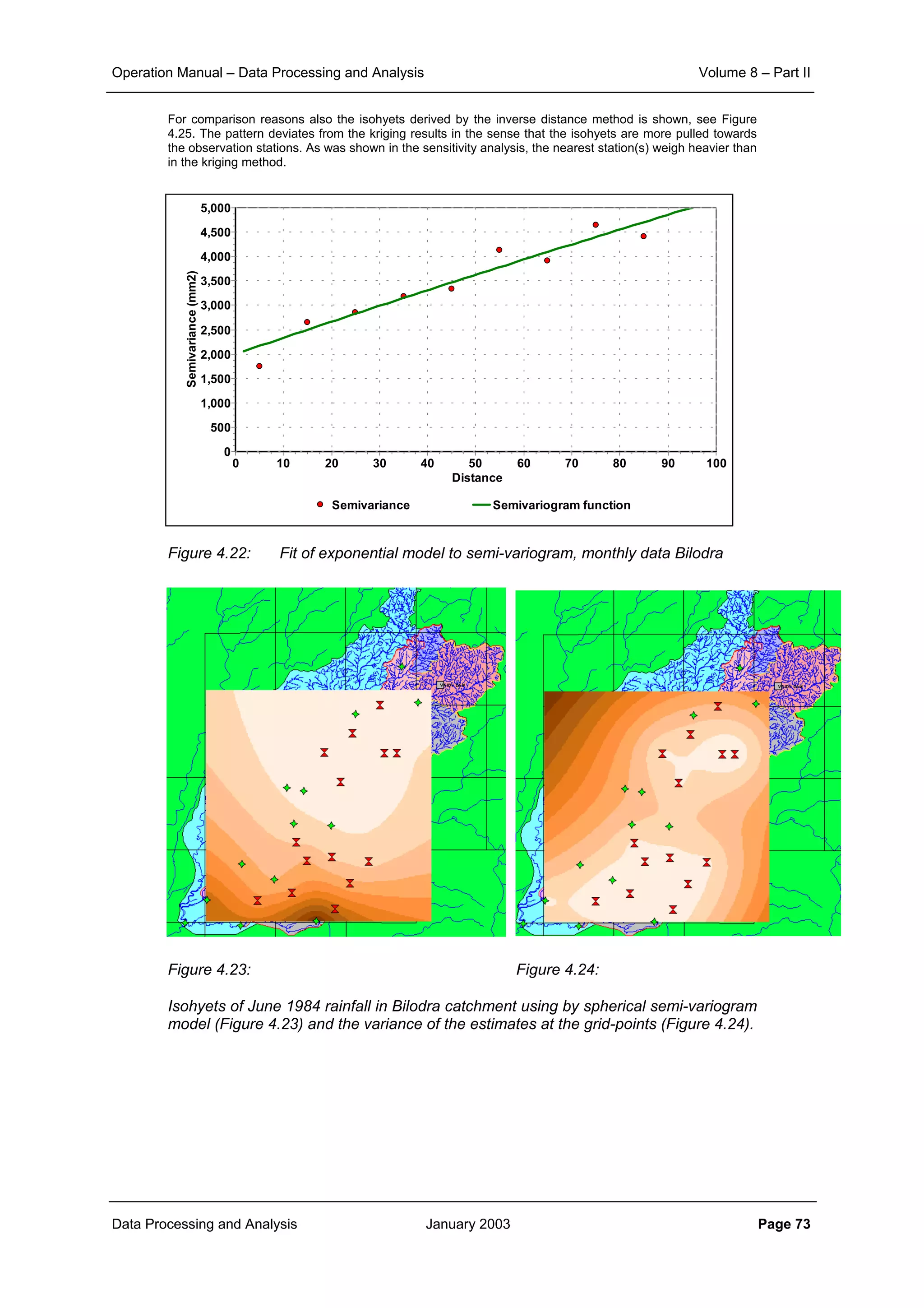
Similarly, the semi-variance was modelled by the exponential model, which in Figure 4.22 is seen to fit in
this case equally well, with parameters C0 = 2,000 mm
2
, Sill = 27,000 mm
2
and Range = 12,00 km. Note
that C0 is considerably smaller than one would expect based on the spatial correlation function, shown in
Figure 4.20. To arrive at the nugget value of 2,000 mm
2
an r0 value of 0.93 would be needed. Important for
fitting the semi-variogram model is to apply an appropriate value for the lag-distance, such that the noise in
the semi-variance is substantially reduced.
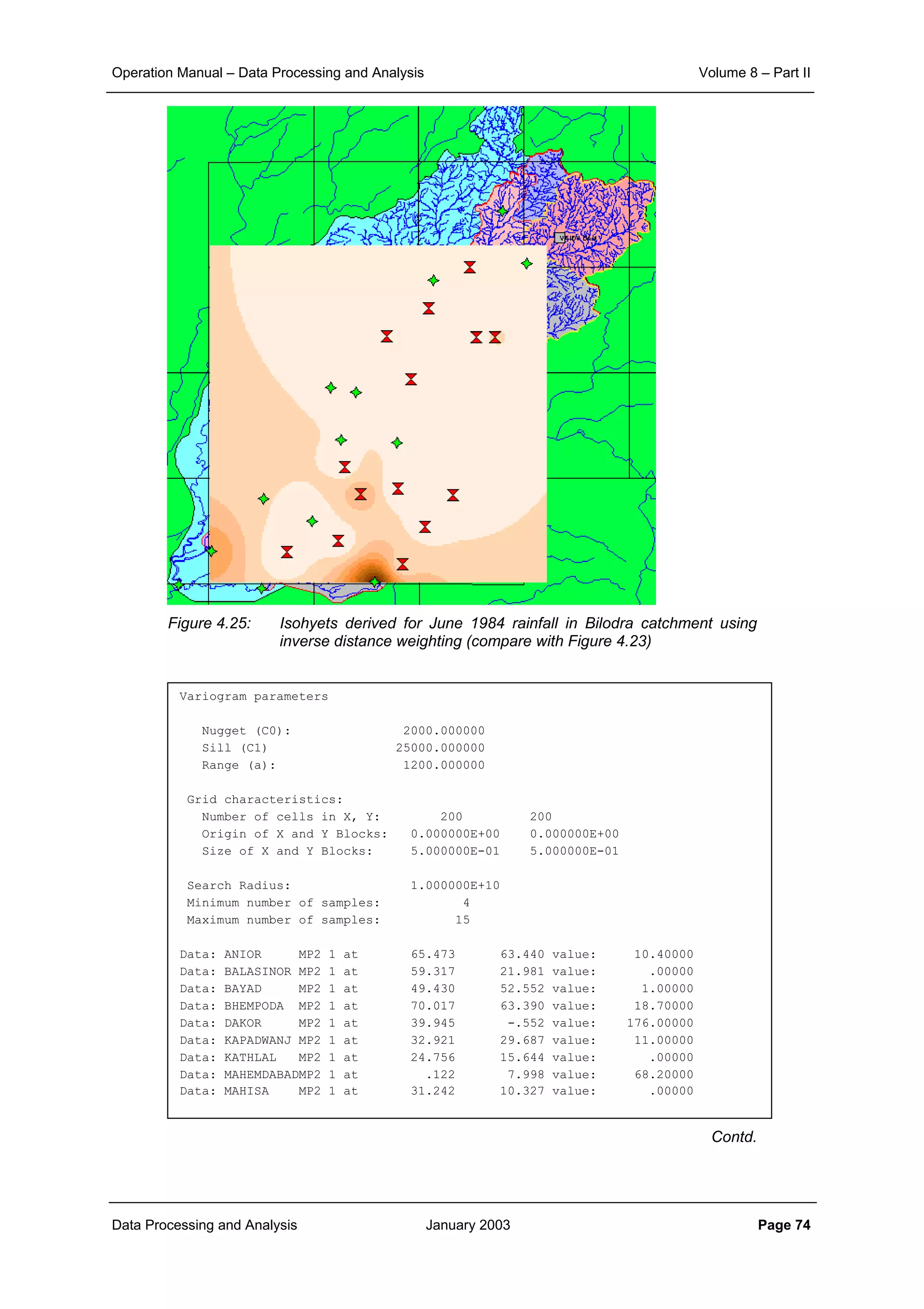
The results with the spherical model applied to the rainfall of June 1984 in the BILODRA catchment is
shown in Figure 4.23. A grid-size of 500 m has been applied. The variance of the estimates is shown in
Figure 4.24. It is observed that the estimation variance at the observation points is zero. Further away from
the observation stations the variance is seen to increase considerably. Reference is made to Table 4.6 for
a tabular output.
Semivariance Semivariogram function
Distance
1,2001,0008006004002000
Semivariance(mm2)
30,000
28,000
26,000
24,000
22,000
20,000
18,000
16,000
14,000
12,000
10,000
8,000
6,000
4,000
2,000
C0 = nugget
Variance
Range
Semivariance Semivariogram function
Distance
1009080706050403020100
Semivariance(mm2)
5,000
4,500
4,000
3,500
3,000
2,500
2,000
1,500
1,000
500
0
Correlation Correlation function
Distance [km]
1009080706050403020100
Correlationcoefficient
1
0.8
0.6
0.4
0.2
0
Details of semi-variance fit](https://image.slidesharecdn.com/download-manuals-surfacewater-manual-swvolume8operationmanualdataprocessingpartii-140509011631-phpapp01/75/Download-manuals-surface-water-manual-sw-volume8operationmanualdataprocessingpartii-77-2048.jpg)


![Operation Manual – Data Processing and Analysis Volume 8 – Part II
Data Processing and Analysis January 2003 Page 123
Standard error expressed in relative terms helps in comparing the extent of fit between the rating
curves for different ranges of discharges. The standard error for the rating curve can be derived for
each segment separately as well as for the full range of data.
Thus 95% of all observed stage discharge data are expected to be within t x Se from the fitted line
where:
Student’s t ≅ 2 where n > 20, but increasingly large for smaller samples.
The stage discharge relationship, being a line of best fit provides a better estimate of discharge than
any of the individual observations, but the position of the line is also subject to uncertainty, expressed
as the Standard error of the mean relationship (Smr) which is given by:
(9.22)
where: t = Student t-value at 95% probability
Pi = ln (hi + a)
S2
P = variance of P
CL 95% = 95% confidence limits
The Se equation gives a single value for the standard error of the logarithmic relation and the 95%
confidence limits can thus be displayed as two parallel straight lines on either side of the mean
relationship. By contrast Smr is calculated for each observation of (h + a). The limits are therefore
curved on each side of the stage discharge relationship and are at a minimum at the mean value of ln
(h + a) where the Smr relationship reduces to:
Smr = ± Se / n1/2
(9.23)
Thus with n = 25, Smr, the standard error of the mean relationship is approximately 20% of Se
indicating the advantage of a fitted relationship over the use of individual gaugings.
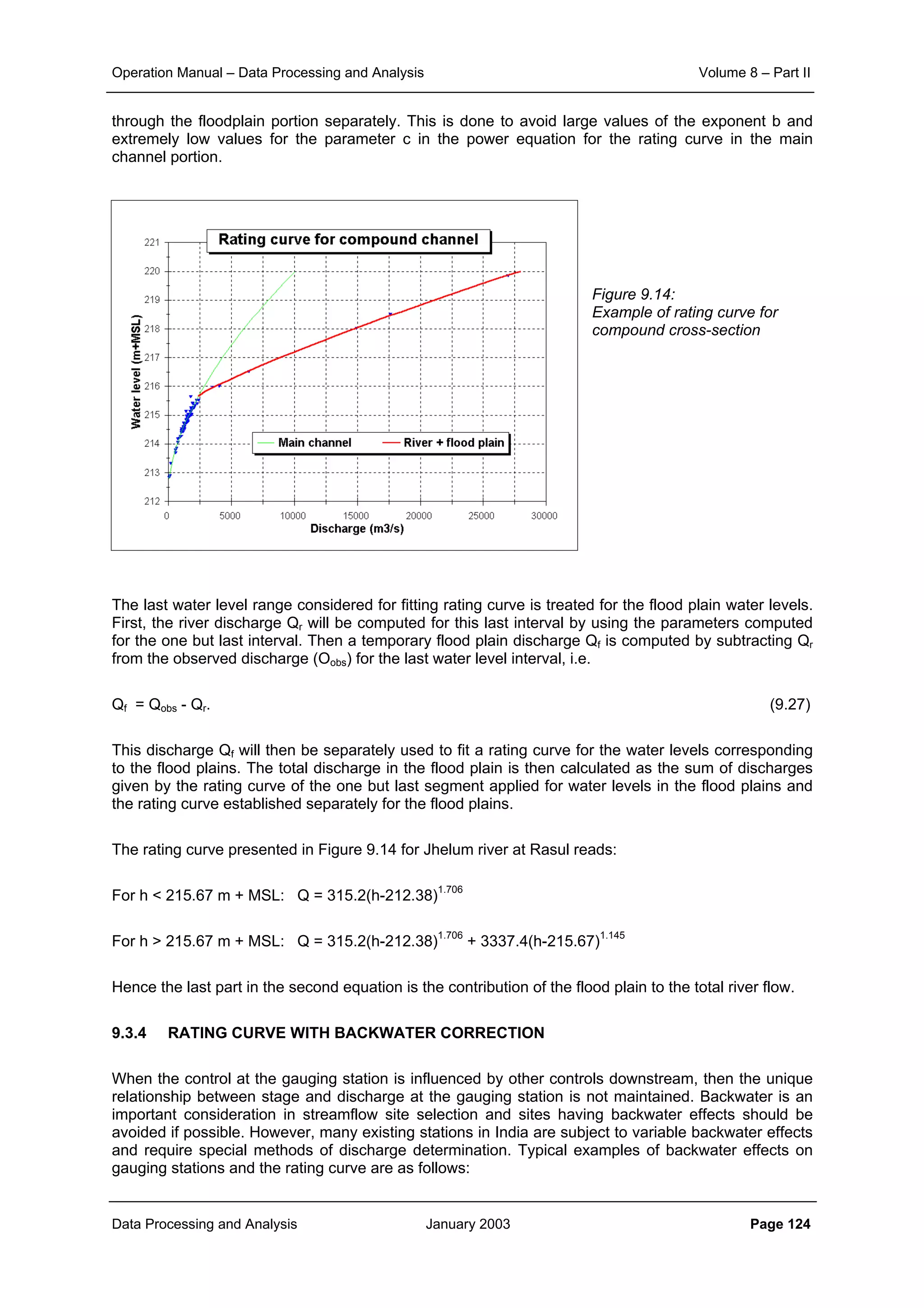
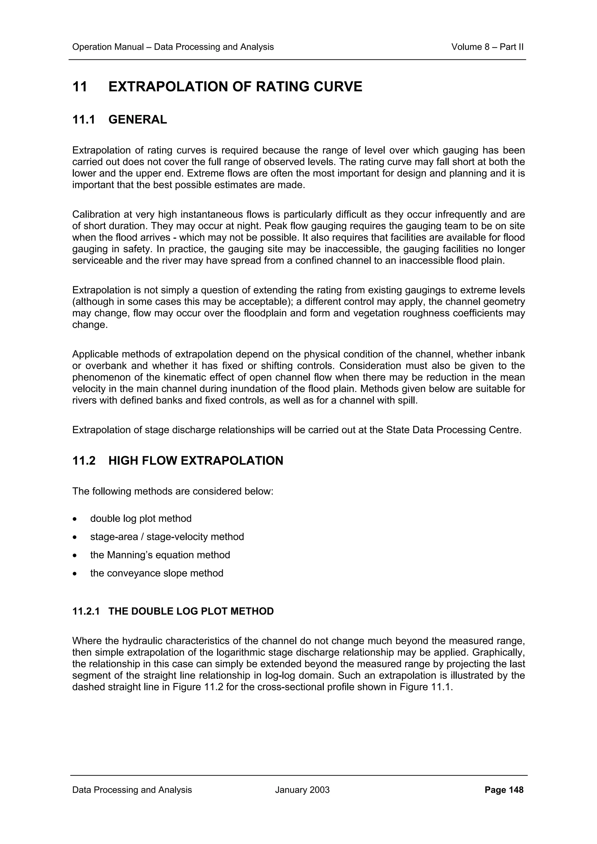
9.3.3 COMPOUND CHANNEL RATING CURVE
If the flood plains carry flow over the full cross section, the discharge (for very wide channels) consists
of two parts:
(9.24)
and
(9.25)
assuming that the floodplain has the same slope as the river bed, the total discharge becomes:
(9.26)
This is illustrated in Figure 9.14. The rating curve changes significantly as soon as the flood plain at
level h-h1 is flooded, especially if the ratio of the storage width B to the width of the river bed Br is
large. The rating curve for this situation of a compound channel is determined by considering the flow
mr%95
2
P
2
i
emr tSCLand
S
)PP(
n
1
SS ±=
−
+=
)ShK()Bh(Q 2/13/2
mrrriver =
]S)hh(K[)BB()hh(Q 2/13/2
1mfr1floodplain −−−=
]S)hh(K[)BB()hh()ShK(BhQ 2/13/2
1mfr1
2/13/2
mrrtotal −−−+=](https://image.slidesharecdn.com/download-manuals-surfacewater-manual-swvolume8operationmanualdataprocessingpartii-140509011631-phpapp01/75/Download-manuals-surface-water-manual-sw-volume8operationmanualdataprocessingpartii-128-2048.jpg)


![Operation Manual – Data Processing and Analysis Volume 8 – Part II
Data Processing and Analysis January 2003 Page 186
will give an unbiased estimate of the average concentration in the vertical. As shown in Sub-section
2.6.3 of the Design Manual of Volume 5 for low values of u*/W a strongy biased result may be
obtained. It is therefore required that for those sites comparisons are being made between
concentrations obtained from concentration measurements over the full depth and the single point
measurements at 0.6 of the depth. To improve the historical data, a correction factor may be
established for the various fractions, to be applied to the old measurements.
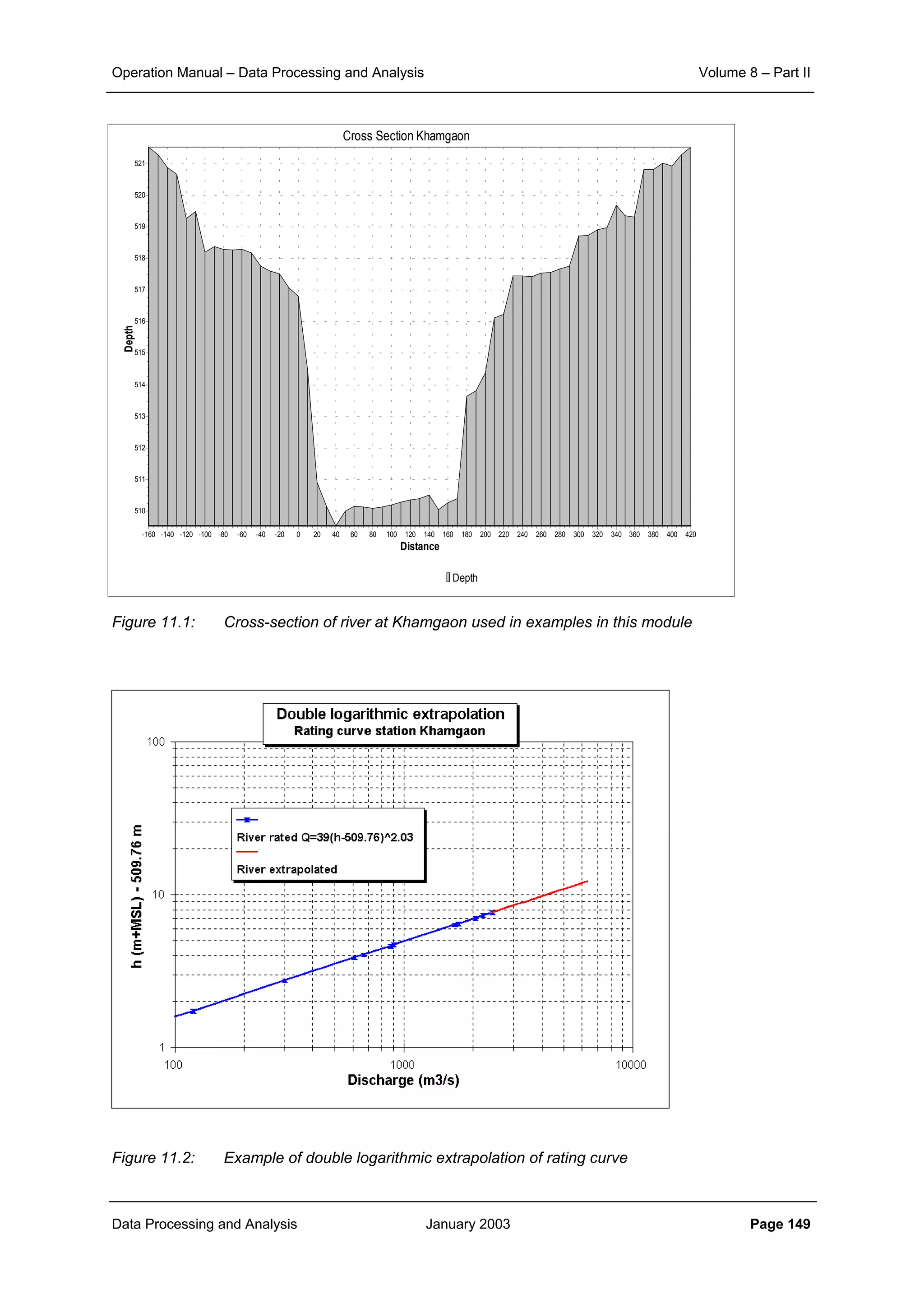
Example 18.1
The total suspended concentrations the test site data used in Chapter 17 for the year 1997 are
displayed in Figure 17.7. From the analysis of the data presented in Chapter 17 it is concluded that:
• a distinct invariable relationship between C+M fractions and discharge exists for the entire
year
• a fairly distinct relationship between the F fraction and discharge is applicable till
September, which drops thereafter. However, in all, the concentration of fines appears to be
small in comparison with the C+M fraction.
Therefore, in view of the small concentration of fines, one relation between total suspended load and
discharge will be established for the year. Hence, the concentration of TSS (Total Suspended
Sediments) is first transformed to total suspended load. Subsequently, a power type relation is
established between discharge and total suspended load for different reaches of the discharge. The
result is shown in Figure 18.1.
Figure 18.1: Fitting of S-Q relation to the total suspended load data for test site
for the year 1997
From the results shown in Figure 18.1, it is seen, that the observed data are well fitted by two
equations:
For Q < 538 m
3
/s: S = 2.74 Q
1.83
[T/d]
For Q 538 m
3
/s: S 210 Q
1.14
[T/d]
Next, the relationships are used to derive the suspended sediment load time series by transformation of the
discharge time series. Still, it has to be determined whether a correction factor has to be applied to arrive at an
unbiased estimate for the sediment load.
Subsequent activities
If the river is entering a reservoir, which is regularly surveyed, a comparison should be made with the
sedimentation rate in the reservoir. For this a percentage has to be added to the suspended load to
account for bed load transport. The match will further be dependent on the trap efficiency of the
reservoir.
1
10
100
1,000
10,000
100,000
1,000,000
10,000,000
1 10 100 1000 10000
Discharge (m
3
/s)
S = 2.74Q
1.83
S = 210Q
1.12](https://image.slidesharecdn.com/download-manuals-surfacewater-manual-swvolume8operationmanualdataprocessingpartii-140509011631-phpapp01/75/Download-manuals-surface-water-manual-sw-volume8operationmanualdataprocessingpartii-191-2048.jpg)


![Vibe Coding vs. Spec-Driven Development [Free Meetup]](https://cdn.slidesharecdn.com/ss_thumbnails/vibecodingvsspecdrivendevelopment-251209105622-43f455e7-thumbnail.jpg?width=640&height=640&fit=bounds)


