This document is Darin Chester Hitchings' PhD dissertation submitted to Boston University. It develops new algorithms for controlling teams of robots performing information-seeking missions in unknown environments with limited sensing budgets. The dissertation first considers scenarios with finite action and measurement spaces and develops algorithms using Lagrangian relaxation and receding horizon control. It then extends these methods to problems with moving objects, continuous action/measurement spaces, and considers how human operators can work with robotic teams. The goal is to maximize information gained about objects while efficiently using limited sensing resources.


![3.4 Bounds for the simulations results in Table 3.3. When the horizon is short,
the 3 MPC algorithms execute more observations per object than were used
to compute the “bound”, and therefore, in this case, the bounds do not match
the simulations; otherwise, the bounds are good. . . . . . . . . . . . . . . . . 46
3.5 Comparison of lower bounds for 2 homogeneous, bi-modal sensors (left 3 columns)
versus 2 heterogeneous sensors in which S1 has only ‘mode1’ available but S2
supports both ‘mode1’ and ‘mode2’ (right 3 columns). There is 1 visibility-
group with πi(0) = [0.7 0.2 0.1]T
∀ i ∈ [0..99]. For many of the cases studied
there is a performance hit of 10–20%. . . . . . . . . . . . . . . . . . . . . . 49
3.6 Comparison of sensor overlap bounds with 2 homogeneous, bi-modal, sensors
and 3 visibility-groups. Both configurations use the prior πi(0) = [0.7 0.2 0.1]T
.
Compare and contrast with the left half of Table 3.5, most of the time the two
sensors have enough objects in view to be able to efficiently use their resources
for both the 60% and 20% overlap configurations; only the bold numbers are
different. . . . . . . . . . . . . . . . . . . . . . . . . . . . . . . . . . . . . 49
3.7 Simulation results for 3 homogeneous sensors without using detection but with
partial overlap as shown in Fig. 3·5. See Fig. 3·6 - Fig. 3·8 for the graphical
version. . . . . . . . . . . . . . . . . . . . . . . . . . . . . . . . . . . . . 51
3.8 Bounds for the simulations results in Table 3.7. When the horizon is short,
the 3 MPC algorithms execute more observations per object than were used to
compute the bound, and therefore, in this case, the bounds do not match the
simulations; otherwise, the bounds are good. . . . . . . . . . . . . . . . . . . 51
5.1 Performance comparison averaged over 100 Monte Carlo simulations. Re-
laxation is the algorithm proposed in this chapter, while Exact is the
algorithm of [Bashan et al., 2008] . . . . . . . . . . . . . . . . . . . . . . 93
xii](https://image.slidesharecdn.com/9f5467db-22a0-4b25-9f85-d66c2d62a6f8-160910233158/85/dissertation-14-320.jpg)
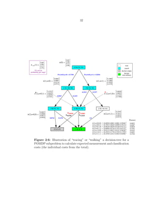
![2·6 Illustration of “tracing” or “walking” a decision-tree for a POMDP sub-
problem to calculate expected measurement and classification costs (the
individual costs from the total). . . . . . . . . . . . . . . . . . . . . . . 32
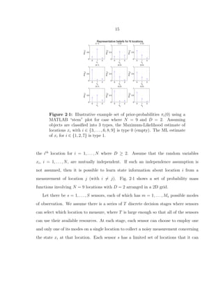
2·7 Strategy 1 (mixture weight=0.726). πi(0) = [0.1 0.6 0.2 0.1]’ ∀ i ∈ [0, . . . , 9],
πi(0) = [0.80 0.12 0.06 0.02]T
∀ i ∈ [10, . . . , 99]. The first 10 objects start with
node 5, the remaining 90 start with node 43. The notation [i Ni0 Ni1 Ni2]
indicates the next node/action from node i as a function of observing the 0th,
1st or 2nd observations respectively. . . . . . . . . . . . . . . . . . . . . . . 33
2·8 Strategy 2 (mixture weight=0.274) πi(0) = [0.1 0.6 0.2 0.1]’ ∀ i ∈ [0, . . . , 9],
πi(0) = [0.80 0.12 0.06 0.02]T
∀ i ∈ [10, . . . , 99]. The first 10 objects start with
node 6, the remaining 90 start with node 18. . . . . . . . . . . . . . . . . 34
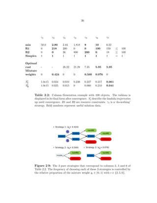
2·9 The 3 pure strategies that correspond to columns 2, 5 and 6 of Table 2.2. The
frequency of choosing each of these 3 strategies is controlled by the relative
proportion of the mixture weight qc ∈ (0..1) with c ∈ {2, 5, 6}. . . . . . . . . 36
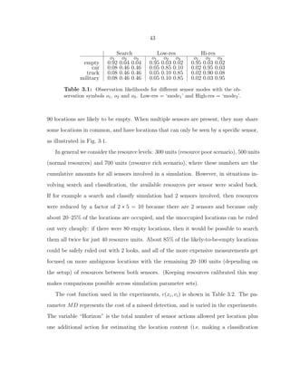
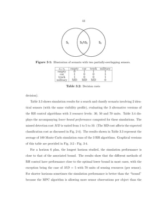
3·1 Illustration of scenario with two partially-overlapping sensors. . . . . . . . . 44
3·2 This figure is the graphical version of Table 3.3 for horizon 3. Simulation results
for two sensors with full visibility and detection (X=’empty’, ’car’, ’truck’, ’mil-
itary’) using πi(0) = [0.1 0.6 0.2 0.1]T
∀ i ∈ [0..9], πi(0) = [0.80 0.12 0.06 0.02]T
∀ i ∈ [10..99]. There is one bar in each sub-graph for each of the three simula-
tion modes studied in this chapter. The theoretical lower bound can be seen
in the upper-right corner of each bar-chart. . . . . . . . . . . . . . . . . . . 47
3·3 This figure is the graphical version of Table 3.3 for horizon 4. . . . . . . . . 47
3·4 This figure is the graphical version of Table 3.3 for horizon 6. . . . . . . . . 48
3·5 The 7 visibility groups for the 3 sensor experiment indicating the number of
locations in each group. . . . . . . . . . . . . . . . . . . . . . . . . . . . . 50
xiv](https://image.slidesharecdn.com/9f5467db-22a0-4b25-9f85-d66c2d62a6f8-160910233158/85/dissertation-16-320.jpg)
![3·6 This figure is the graphical version of Table 3.7 for horizon 3. Situation with
no detection but limited visibility (X=’car’, ’truck’, ’military’) using πi(0) =
[0.70 0.20 0.10]T
∀ i ∈ [0..99]. There were 7 visibility-groups: 20x001, 20x010,
20x100, 12x011, 12x101, 12x110, 4x111. The 3 bars in each sub-graph are for
‘str1’, ‘str2’, ‘str3’ respectively. The theoretical lower bound can be seen in the
upper-right corner of each bar-chart. . . . . . . . . . . . . . . . . . . . . . 52
3·7 This figure is the graphical version of Table 3.7 for horizon 4. . . . . . . . . 52
3·8 This figure is the graphical version of Table 3.7 for horizon 6. . . . . . . . . 53
4·1 An example HMM that can be used for each of the N locations. pa is an
arrival probability and pd is a departure probability for the Markov chain. 57
5·1 Depiction of measurement likelihoods for empty and non-empty cells as a func-
tion of xk0.
√
xk0 gives the mean of the density p(Yk0|Ik = 1). If the cell is
empty the observation is always mean 0 (black curve). . . . . . . . . . . . . 74
5·2 Waterfall plot of joint probability p(Yk0|Ik; xk0) for πk0 = 0.50 for xk0 ∈
[0 . . . 20]. This figure shows the increased discrimination ability that results
from using higher-energy measurements (separation of the peaks). . . . . . . 75
5·3 Graphic showing the posterior probability πk1 as a function of the initial ac-
tion xk0 and the initial measurement value Yk0. This surface plot is for λ = 0.01
and πk0 = 0.20. (The boundary between the high (red) and low (blue) portions
of this surface is not straight but curves towards -y with +x.) . . . . . . . . 76
5·4 Cost function boundary (see Eq. 5.14) with λ = 0.011 and πk0 = 0.18. In the
lighter region two measurements are made, in the darker region just one. (Note
positive y is downwards.) . . . . . . . . . . . . . . . . . . . . . . . . . . . 80
xv](https://image.slidesharecdn.com/9f5467db-22a0-4b25-9f85-d66c2d62a6f8-160910233158/85/dissertation-17-320.jpg)
![5·5 The optimal boundary for taking one action or two as a function of (xk0, Yk0)
(for the [Bashan et al., 2008] cost function) for λ = 0.01 and πk0 = 0.20. The
curves in Fig. 5·6 represent cross-sections through this surface for the 3 x-values
referred to in that figure. . . . . . . . . . . . . . . . . . . . . . . . . . . . 80
5·6 This figure gives another depiction of the optimal boundary between taking
one measurement action or two for the [Bashan et al., 2008] cost function. For
all Y (xk0, λ) ≥ 0 two measurements are made (and the highest curve is for the
smallest xk0, see Fig. 5·5 for the 3D surface from which these cross-sections
were taken). . . . . . . . . . . . . . . . . . . . . . . . . . . . . . . . . . . 81
5·7 Two-factor exploration to determine how the optimal boundary between taking
one measurement or two measurements varies for a cell with the parameters
(p, λ) where p = πk0 (for the [Bashan et al., 2008] problem cost function). Two
measurements are taken in the darker region, one measurement for the lighter
region. . . . . . . . . . . . . . . . . . . . . . . . . . . . . . . . . . . . . . 82
5·8 Plot of cost function samples associated with false alarms, missed detections
and the optimal choice between false alarms and missed detections (for the
Bayes’ cost function). . . . . . . . . . . . . . . . . . . . . . . . . . . . . . 85
5·9 This figure shows cost-to-go function samples as a function of the second
sensing-action xk1 and the second measurement Yk1 for the Bayes’ cost func-
tion. These plots use 1000 samples for Yk1 and 100 for xk1. . . . . . . . . . . 87
5·10 Threshold function for declaring a cell empty (risk of MD) or occupied (risk of
FA). . . . . . . . . . . . . . . . . . . . . . . . . . . . . . . . . . . . . . . 88
5·11 The 0th stage resource allocation as a function of prior probability. The stria-
tions are an artifact of the discretization of resources when looking for optimal
xk0. . . . . . . . . . . . . . . . . . . . . . . . . . . . . . . . . . . . . . . 90
xvi](https://image.slidesharecdn.com/9f5467db-22a0-4b25-9f85-d66c2d62a6f8-160910233158/85/dissertation-18-320.jpg)
![5·12 Total resource allocation to a cell as a function of prior probability. The point-
wise sums of the 0th stage and 1st stage resource expenditures are displayed
here. . . . . . . . . . . . . . . . . . . . . . . . . . . . . . . . . . . . . . . 91
5·13 Cost associated with a cell as a function of prior probability. For the optimal
resource allocations, there is a one-to-one correspondence between the cost of
a cell and the resource utilized to sense a cell. . . . . . . . . . . . . . . . . 92
5·14 Cost-to-go from πk1 . . . . . . . . . . . . . . . . . . . . . . . . . . . . . . 93
5·15 Optimal stage 1 energy allocations. . . . . . . . . . . . . . . . . . . . . . . 94
5·16 Stage 0 energy allocation versus prior probability . . . . . . . . . . . . . . . 95
6·1 Graphical User Interface (GUI) concept for semi-autonomous search and
exploitation strategy game. . . . . . . . . . . . . . . . . . . . . . . . . . 106
A·1 Hyperplanes representing the optimal Value Function (cost framework)
for the canonical Wald Problem [Wald, 1945] with horizon 3 (2 sensing
opportunities and a declaration) for the equal missed detection and false
alarm cost case: FA=MD. . . . . . . . . . . . . . . . . . . . . . . . . . . 119
A·2 Decision-tree for the Wald Problem. This figure goes with Fig. A·1. . . . 119
A·3 Example of 3D hyperplanes for a value function (using a reward formu-
lation for visual clarity) for X = {‘military’,‘truck’,‘car’,‘empty’}, S = 1,
M = 3 for a horizon 3 problem. The cost coefficients for the non-military
vehicles were added together to create the 3D plot. This figure and
Fig. A·4 are a mixed-strategy pair. . . . . . . . . . . . . . . . . . . . . . 122
A·4 Example of 3D hyperplanes representing the optimal value function re-
turned by Value Iteration. The optimal value is the convex hull of these
hyperplanes. This figure and Fig. A·3 are a mixed-strategy pair (see
Section 2.3). . . . . . . . . . . . . . . . . . . . . . . . . . . . . . . . . . 123
xvii](https://image.slidesharecdn.com/9f5467db-22a0-4b25-9f85-d66c2d62a6f8-160910233158/85/dissertation-19-320.jpg)


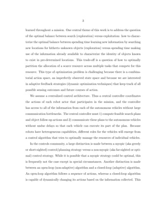
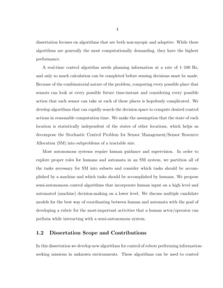
![5
multiple, multi-modal, resource-constrained sensors on autonomous vehicles by specify-
ing where and how they should be used to maximize one of several possible performance
metrics for the mission. The goals of the mission are application-dependent, but at the
very least they will include accurately locating, observing and classifying objects in the
mission space.
The SM control problem can be formulated as a Partially Observed Markov Decision
Problem (POMDP), but its exact solution requires excessive computation. Instead, we
use Lagrangian Relaxation techniques to decompose the original SM problem hierarchi-
cally into POMDP subproblems with coupling constraints and a master problem that
coordinates the prices of resources. To this end, this dissertation makes the following
contributions:
• Develops a Column Generation algorithm that creates mixed strategies for SM and
implements this algorithm in fast, C language code. This algorithm creates sensor plans
that near-optimally solve an approximation of the original SM problem, but generates
mixed strategies that may not be feasible. The output strategies are programmatically
visualized in MATLAB.
• Develops alternatives for receding horizon control using these approximate, mixed strate-
gies output from the Column Generation routine, and evaluates their performance using
a fractional factorial design of experiments based on the above software.
• Extends previous results in SM for classification of stationary objects to allow Markov
dynamics and time varying visibility, obtaining new lower bounds characterizing achiev-
able performance for these problems. These lower bounds can be used to develop receding
horizon control strategies.
• Develops new approaches for solution of dynamic search problems with continuous ac-
tion and observation spaces that are much faster than previous optimal results, with
near-optimal performance. We perform simulations of our algorithms in MATLAB and
compare our results with those of the optimal algorithm from [Bashan et al., 2007,Bashan
et al., 2008]. Our algorithm performs similarly to theirs but can be used for problems
with non-uniform priors.
• Designs a game to explore human supervisory control of automata controlled by our](https://image.slidesharecdn.com/9f5467db-22a0-4b25-9f85-d66c2d62a6f8-160910233158/85/dissertation-27-320.jpg)
![6
algorithms, in order to explore the effects of different levels of information support on
the quality of supervisory control.
1.3 Dissertation Organization
The structure of the remainder of this dissertation is as follows: Chapter 2 is devoted
to presenting a literature survey and background material that is pertinent to the SM
problem. Chapter 2 also reviews theory from [Casta˜n´on, 2005b] that underlies the
theoretical foundations of this dissertation’s results. Chapter 3 builds upon the results
of Chapter 2 and discusses a RH algorithm for near-optimal SM in a scenario where
objects have static state and sensor platforms are unconstrained in terms of where they
look and when (no motion constraints). Chapter 4 discusses new algorithms for two
extensions to the problem formulation of Chapter 3: 1) objects that can arrive and
depart with a Markov birth-death process or 2) object visibility that is known but time-
varying. Chapter 5 considers an adaptive search problem for sensors with continuous
action and observation spaces and presents fast, near-optimal algorithms for the solution
of these problems. Chapter 6 discusses some candidate strategies for mixed human/non-
human, semi-autonomous robotic search and exploit teams and develops a game that can
be used to explore human supervisory control of robotic teams. Chapter 7 summarizes
this dissertation. Last of all, two appendices are included that provide some additional
background theory and documentation for the simulator discussed in Chapter 3.](https://image.slidesharecdn.com/9f5467db-22a0-4b25-9f85-d66c2d62a6f8-160910233158/85/dissertation-28-320.jpg)
![7
Chapter 2
Background
This chapter provides both a literature survey and background material that will be
referred to in later chapters. First we review existing techniques from various fields
related to this dissertation. We describe why the algorithms presented in the litera-
ture fail to address the problem we envision to the extent that is required for a search
and exploitation system to be considered “semi-autonomous”, which we take to mean
an Autonomous Capability Level (ACL) of 6 or higher on the DoDs “UAV Roadmap
2009” [United States Department of Defense, 2009]. Section 2.2 discusses the develop-
ment of a lower bound for the achievable performance of a SM system from [Casta˜n´on,
2005b]. The last section in this chapter, Section 2.3, gives an example of our algo-
rithm for computing SM plans. The implementation of the algorithm from [Casta˜n´on,
2005b], as demonstrated by this example, is the first contribution of this dissertation.
For the interested reader, a brief review of theory pertaining to Partially Observable
Markov Decision Processes (POMDPs), the Witness Algorithm and Point-Based Value
Iteration (PBVI), Dantzig-Wolfe Decompositions and Column Generation is available
in Appendix A.
2.1 Literature Survey
Problems of search and exploitation have been considered in many fields such as Search
Theory, Information-Theory, Multi-armed Bandit Problems (MABPs), Stochastic Con-
trol, and Human-Robot Interactions. We will review relevant results in each of these](https://image.slidesharecdn.com/9f5467db-22a0-4b25-9f85-d66c2d62a6f8-160910233158/85/dissertation-29-320.jpg)
![8
areas in the rest of this section.
2.1.1 Search Theory
One of the earliest examples of Sensor Management (SM) arose in the context of Search,
with application to anti-submarine warfare in the 1940’s [Koopman, 1946, Koopman,
1980]. In this context, Search Theory was used to characterize the optimal allocation
of search effort to look for a single stationary object with a single imperfect sensor.
Sensors had the ability to move spatially and allocate their search effort over time and
space. In [Koopman, 1946] a worst-case search-performance rule is derived yielding the
“Random Search Law” aka the “Exponential Detection Function” [Stone, 1977]. This
work is extended in [Stone, 1975] to handle the case of a single moving object. A survey
of the field of Search Theory is given by [Benkoski et al., 1991], which describes how
most work in this domain focuses on open-loop search plans rather than feedback control
of search trajectories.
The main problem with most Search Theory results is that the search strategies are
non-adaptive and the search ends after the object has been found. Extensions of Search
Theory to problems requiring adaptive feedback strategies have been developed in some
restricted contexts [Casta˜n´on, 1995] where a single sensor takes one action at a time.
Recent work on Search has focused on deterministic control of search vehicle tra-
jectories using different performance metrics. Baronov et al. [Baillieul and Baronov,
2010,Baronov and Baillieul, 2010] describe an information aquisition algorithm for the
autonomous exploration of random, continuous fields in the context of environmental
exploration, reconaissance and surveillance. Our focus in this thesis is on adaptive
sensor scheduling based on noisy observations, and not on control of sensor-platform
trajectories.](https://image.slidesharecdn.com/9f5467db-22a0-4b25-9f85-d66c2d62a6f8-160910233158/85/dissertation-30-320.jpg)
![9
2.1.2 Information Theory for Adaptive Sensor Management
Adaptive SM has its roots in the field of statistics, in which Bayesian experiment design
was used to configure subsequent experiments that were based on observed information.
Wald [Wald, 1943,Wald, 1945] considered sequential hypothesis testing with costly ob-
servations. Lindley [Lindley, 1956] and Kiefer [Kiefer, 1959] expanded the concepts
to include variations in potential measurements. Chernoff [Chernovv, 1972] and Fe-
dorov [Fedorov, 1972] used Cramer-Rao bounds for selecting sequences of measurements
for nonlinear regression problems. Most of the strategies proposed for Bayesian experi-
ment design involve single-step optimization criteria, resulting in “greedy” (or “myopic”)
strategies that optimize bounds on the expected performance after the next experiment.
Athans [Athans, 1972] considered a two-point boundary value approach to controlling
the error covariance in linear estimators by choosing the measurement matrices. Other
approaches to adaptive SM using single-stage optimization have been proposed with al-
ternative information theoretic measures [Schmaedeke, 1993,Schmaedeke and Kastella,
1994,Kastella, 1997,Kreucher et al., 2005].
Most of the work on information theory approaches for SM is focused on tracking
objects using linear or nonlinear estimation techniques [Kreucher et al., 2005,Wong et al.,
2005,Grocholsky, 2002,Grocholsky et al., 2003] and use myopic (single stage) policies.
Myopic policies generated by entropy-gain criteria perform well in certain scenarios,
but they have no guarantees for optimality in dynamic optimization problems. Along
these lines, the dissertation by Williams provides a set of performance bounds on greedy
algorithms as compared to optimal closed-loop policies in certain situations [Williams,
2007].](https://image.slidesharecdn.com/9f5467db-22a0-4b25-9f85-d66c2d62a6f8-160910233158/85/dissertation-31-320.jpg)
![10
2.1.3 Multi-armed Bandit Problems
In the 1970s [Gittins, 1979] developed an optimal indexing rule for “Multi-armed Bandit
Problems” (MABP) that is applicable to SM problems. In these approaches, different
objects are modeled as ”bandits” and assigning a sensor to look at an object is equivalent
to playing the ”bandit”, thereby changing the ”bandit’s” state. Krishnamurthy et al.
[Krishnamurthy and Evans, 2001a,Krishnamurthy and Evans, 2001b] and Washburn et
al. [Washburn et al., 2002] use MABP models to obtain SM policies for tracking moving
objects. The MABP model limits their work to policies that use a single sensor with a
single mode, so only one object can be observed at a time.
2.1.4 Stochastic Control
Stochastic control approaches to SM problems are often posed as Stochastic Control
Problems and solved using Dynamic Programming techniques [Bertsekas, 2007]. Evans
and Krishnamurthy [Krishnamurthy and Evans, 2001a] use a Hidden Markov Model
(HMM) to represent object dynamics while planning sensor schedules. Using a Stochas-
tic Dynamic Programming (SDP) approach, optimal policies are found for the cost
functions studied. While the proposed algorithm provides optimal sensor schedules for
multiple sensors, it only deals with one object.
Several authors have recently proposed approximate Stochastic Dynamic Program-
ming techniques for SM based on value function approximations or reinforcement learn-
ing [Wintenby and Krishnamurthy, 2006,Kreucher and Hero, 2006,Chong et al., 2008a,
Washburn et al., 2002,Schneider et al., 2004,Williams et al., 2005,Chong et al., 2008a,
Chong et al., 2008b]. The majority of these results are focused on the problem of track-
ing objects. Furthermore, the proposed approaches are focused on small numbers of
objects, and fail to address the range and scale of the problems of interest in this dis-
sertation. A good overview of approximate DP techniques is available in [Casta˜n´on and](https://image.slidesharecdn.com/9f5467db-22a0-4b25-9f85-d66c2d62a6f8-160910233158/85/dissertation-32-320.jpg)
![11
Carin, 2008].
Bashan, Reich and Hero [Bashan et al., 2007, Bashan et al., 2008] use DP to solve
a class of two-stage adaptive sensor allocation problems for search with large numbers
of possible cells. The complexity of their algorithm restricts its application to problem
classes where every cell has a uniform prior. Similar results were obtained for an imaging
problem in [Rangarajan et al., 2007]. In this thesis, we develop a different approach that
overcomes this limitation in Ch. 5.
In [Yost and Washburn, 2000], Yost describes a hierarchical algorithm for resource
allocation using a Linear Program (LP) at the top level (the “master problem”) to
coordinate a set of POMDP subproblems in a Battle Damage Assessment (BDA) setting.
This work is similar to the approach of this dissertation, except we are concerned with
more complicated POMDP subproblems.
The problem of unreliable resource allocation is discussed in [Casta˜n´on and Wohletz,
2002,Castanon and Wohletz, 2009] in which a pool of M resources is assigned to complete
N failure-prone tasks over several stages using an SDP formulation. Casta˜n´on proposes
a receding-horizon control approach to solve a relaxed DP problem that has an execution
time nearly linear in the number of tasks involved, however this work does not handle a
partially observable state.
Most approaches for dynamic feedback control are limited in application to problems
with a small number of sensor-action choices and simple constraints because the algo-
rithms must enumerate and evaluate the various control actions. In [Casta˜n´on, 1997],
combinatorial optimization techniques are integrated into a DP formulation to obtain
approximate SDP algorithms that extend to large numbers of sensor actions. Subsequent
work in [Casta˜n´on, 2005b] derives an SDP formulation using partially observed Markov
decision processes (POMDPs) and obtains a computable lower bound to the achievable
performance of feedback strategies for complex multi-sensor, SM problems. The lower](https://image.slidesharecdn.com/9f5467db-22a0-4b25-9f85-d66c2d62a6f8-160910233158/85/dissertation-33-320.jpg)
![12
bound is obtained by a convex relaxation of the original combinatorial POMDP using
mixed strategies and averaged constraints. However, the results in [Casta˜n´on, 2005b]
do not specify algorithms with performance close to the lower bound (see Section 2.2).
This dissertation describes such an algorithm in Ch. 3 and then proposes theoretical
extensions to this algorithm in Ch. 4.
2.1.5 Human-Robot Interactions and Human Factors
The use of simulation as a technique to explore the best means of Human-Robot Inter-
action (HRI) in teams with multiple robots per human is the subject of [Dudenhoeffer
et al., 2001]. Questions of human situational awareness, mode awareness (what the
robot is currently doing), and mental model formulation are discussed.
In [Raghunathan and Baillieul, 2010], a search game involving the identification
of roots of random polynomials is presented. The paper analyses the search versus
exploration trade-off made by players and develops Markov models that emulate the
style of play of the 18 players involved in the experiments indistinguishably w.r.t. a
performance metric.
The SAGAT tool for measuring situational awareness has gained wide acceptance in
the literature [Endsley, 1988]. This tool is important for estimating an operator’s ability
to adequately control a team of robots and avoid mishaps.
In the M.S. thesis of [Anderson, 2006], various hierarchical control structures are
described for the human control of multiple robots. A game of tag is played inside
a maze by two teams of three robots controlled at 5 levels of autonomy, and various
metrics for human and robot performance are studied. Robots in this work are either
tele-operated or move myopically, and sensor measurements are noiseless within a certain
range.
In [Scholtz, 2002], possible HRI interactions are divided up into three categories, and](https://image.slidesharecdn.com/9f5467db-22a0-4b25-9f85-d66c2d62a6f8-160910233158/85/dissertation-34-320.jpg)
![13
it is speculated that each category of interaction requires different types of information
and a different interface. This work suggests that a system with multiple levels of
autonomy requires different kinds kind of interfaces according to its mode of operation
and needs to be able to transition between them without confusing the human operator.
In [Cummings et al., 2005], Cummings discusses a list of issues that need to be
addressed to achieve the military’s vision for Network Centric Warfare (NCW). The
author states that to improve system performance, systems must move from a paradigm
of Management by Consent (MBC) to Management by Exception (MBE).
A system for predicting human performance in tasking multiple robotic vehicles is
discussed in [Crandall and Cummings, 2008]. Human behavior is predicted by generating
several stochastic models for 1) the amount of time humans need to issue commands
and 2) the amount of time humans need to switch between tasks. Several performance
metrics are also presented for situational awareness, for the effectiveness of an operator’s
communications with a robot, and for the success of robot behavior while untasked.
These references for HRI focus on human situational awareness, performance metrics,
and various control strategies for human control of automata in simple environments.
These references do not investigate the question of an optimal means of HRI in a semi-
autonomous system in which robots with noisy, resource-constrained sensors are used to
explore an unknown, partially-observable and dynamic environment using non-myopic
and adaptive search strategies.
2.1.6 Summary of Background Work
As the above discussion indicates, the research to date has focused on only parts of
the problem of interest in this dissertation. The methods used in the existing body
of research need to be merged and unified in an intelligent fashion such that a semi-
autonomous search, plan, and execution system is created that behaves cohesively and](https://image.slidesharecdn.com/9f5467db-22a0-4b25-9f85-d66c2d62a6f8-160910233158/85/dissertation-35-320.jpg)
![14
in a non-myopic, adaptive fashion.
In this dissertation, we develop and implement algorithms for the efficient compu-
tation of adaptive SM strategies for complex problems involving multiple sensors with
different observation modes and large numbers of potential object locations. The al-
gorithms we present are based on using the lower bound formulation from [Casta˜n´on,
2005b] as an objective in a RH optimization problem and on developing techniques for
obtaining feasible sensing actions from (generally infeasible) mixed strategy solutions.
These algorithms support the use of multiple, multi-modal, resource-constrained, noisy
sensors operating in an unknown environment in a search and classification context.
The resulting near-optimal, adaptive algorithms are scalable to large numbers of tasks,
and suitable for real-time SM.
2.2 Sensor Management Formulation and Previous Results
In this section, we discuss the SM stochastic control formulation and results presented
in [?] which serve as the starting point for our work in subsequent chapters. We extend
the notation of [?] to include multiple sensors and additional modes such as search.
2.2.1 Stationary SM Problem Formulation
Assume there are a finite number of locations 1, . . . , N, each of which may have an object
with a given type, or which may be empty. Assume that there is a set of S sensors, each
of which has multiple sensor modes, and that each sensor can observe one and only one
location at each time with a selected mode. This assumption can be relaxed, although
it introduces additional complexity in the exposition and the computation.
Let xi ∈ {0, 1, . . . , D} denote the state of location i, where xi = 0 if location i
is unoccupied, and otherwise xi = k > 0 indicates location i has an object of type
k. Let πi(0) ∈ ℜD+1
be a discrete probability distribution over the possible states for](https://image.slidesharecdn.com/9f5467db-22a0-4b25-9f85-d66c2d62a6f8-160910233158/85/dissertation-36-320.jpg)
![16
observe, denoted by Os ⊆ {1, . . . , N}. A sensor action by sensor s at stage t is a pair:
us(t) = (is(t), ms(t)) (2.1)
consisting of a location to observe, is(t) ∈ Os, and a mode for that observation, ms(t).
Sensor measurements by sensor s with mode m at stage t, ys,m(t) are modeled as be-
longing to a finite set ys,m(t) ∈ {1, . . . , Ls}. The conditional probability of the measured
value is assumed to depend on the sensor s, sensor mode m, location i and on the true
state at the location, xi, but not on the states of other locations. Denote this condi-
tional probability as P(ys,m(t)|xi, i, s, m). We assume that this conditional probability
given xi is time-invariant, and that the random measurements ys,m(t) are conditionally
independent of other measurements yσ,n(τ) given the states xi, xj for all sensors s, σ
and modes m, n provided i = j or τ = t.
Each sensor has a limited quantity of Ri resources available for measurements over
the T stages of time. Associated with the use of mode m by sensor s on location i is
a resource cost rs(us(t)) to use this mode, representing power or some other type of
resource required to use this mode from this sensor.
T−1
t=0
rs(us(t)) ≤ Rs ∀ s ∈ [1, . . . , S] (2.2)
This is a hard constraint for each realization of observations and decisions.
Let I(t) denote the history of past sensing actions and measurement outcomes up to
and including stage t − 1:
I(t) = {(us(τ), ys,m(τ)), s = 1, . . . , S; τ = 0, . . . , t − 1}
As is frequently the case when working with POMDPs, we make use of the idea of the
information history as a sufficient statistic for the state of the system/world x.](https://image.slidesharecdn.com/9f5467db-22a0-4b25-9f85-d66c2d62a6f8-160910233158/85/dissertation-38-320.jpg)
![17
Under the assumption of conditional independence of measurements and indepen-
dence of individual states at each location, the joint probability π(t) = P(x1 = k1, x2 =
k2, . . . , xN = kN |I(t)) can be factored as the product of belief-states (marginal condi-
tional probabilities) for each location. Denote the conditional probability (belief-state)
at location i as πi(t) = p(xi|I(t)). The probability vector π(t) is a sufficient statistic for
all information that is known about the state of the N locations up until time t.
When a sensor measurement is taken, the belief-state π(t) is updated according to
Bayes’ Rule. A measurement of location i with the sensor-mode combination us(t) =
(i, m) at stage t that generates observable ys,m(t) updates the belief-vector as:
πi(t + 1) =
diag{P(ys,m(t)|xi = j, i, s, m)}πi(t)
1T
diag{P(ys,m(t)|xi = j, i, s, m)}πi(t)
(2.3)
where 1 is the D + 1 dimensional vector of all ones. Eq. 2.3 captures the relevant
information dynamics that SM controls. For generality, the index i in the likelihood
function specifies that the sensor statistics could vary on a location-by-location basis.
Of prime importance is the fact that using π(t) as a sufficient statistic along with
Eq. 2.3, we are able to combine a priori probabilities represented by π(t) with conditional
probabilities given by sensor measurements in order to form posterior probabilities,
π(t + 1), in recursive fashion: beliefs can be maintained and propagated.
In addition to information dynamics, there are resource dynamics that characterize
the available resources at stage t. The dynamics for sensor s are given as:
Rs(t + 1) = Rs(t) − rs(us(t)); Rs(0) = Rs (2.4)
These dynamics constrain the admissible decisions by a sensor, in that it can only use
modes that do not use more resources than are available.
An adaptive feedback strategy is a closed-loop policy or decision-making rule that
maps collected information sets up until stage t, i.e. the sets Ii(τ) ∀ i ∈ [1, . . . , N], τ ∈](https://image.slidesharecdn.com/9f5467db-22a0-4b25-9f85-d66c2d62a6f8-160910233158/85/dissertation-39-320.jpg)
![18
[0, . . . , t − 1] to choose actions for stage t: γ : I(t) → U(t). Define a local strategy, γi,
as an adaptive feedback strategy that chooses actions for location i purely based on the
information sets Ii(t), which is to say based purely on the history of past actions and
observations specific to location i.
Given the final information, I(T), the quality of the information collected is measured
by making an estimate of the state of each location i given the available information.
Denote these estimates as vi ∀ i = 1, . . . , N. The Bayes’ cost of selecting estimate vi
when the true state is xi is denoted as c(xi, vi) ∈ ℜ with c(xi, vi) ≥ 0. The objective of
the SM stochastic control formulation is to minimize:
J =
N
i=1
E[c(xi, vi)] (2.5)
by selecting adaptive sensor control policies and final estimates subject to the dynamics
of Eq. 2.3 and the constraints of Eq. 2.2 and Eq. 2.4.
This problem was solved using dynamic programming in [Casta˜n´on, 2005a] as follows:
Define the optimal value function V (π, R, t) that is the optimal solution to Eq. 2.5
subject to Eq. 2.2 and Eq. 2.4 when the initial information is π, and R is the vector
of current resource levels. Let R = [R1 R2 . . . RS]T
. Define πij as the jth
component
of the probability vector associated with location i. The value function is defined on
SN
× ℜS
+. Let U represent the set of all possible sensor actions and define U(R) ⊂ U
as the set of feasible actions with resource level R. The value function V (π, R, t) must
be recursively related to V (π, R, t + 1), its value one time step earlier, according to
Bellman’s Equation [Bellman, 1957]:
V (π, R, t + 1) = min
N
i=1
min
vi∈X
j=0,...,D
c(j, vi)πij, (2.6)
min
u∈U(R)
E
y
{V (T(π, u, y), R − Ru, t)}](https://image.slidesharecdn.com/9f5467db-22a0-4b25-9f85-d66c2d62a6f8-160910233158/85/dissertation-40-320.jpg)
![19
where Ru = [r1(u1(t)) r2(u2(t)) . . . rS(uS(t))]T
and T(.) is an operator describing the
belief dynamics. T is the identity mapping for information states πj(t) ∀ j except for
{j | j = is ∀ s ∈ [1, . . . , S]}, the set of sensed locations. For a sensed location i, T maps
πi(t) to πi(t + 1) with Eq. 2.3. The expectation in Eq. 2.6 is given by:
E
y
{V (T(π, u, y), R − Ru, t)} =
y∈Ys,m ∀ s
P(y|I(k), u)V (T(π, u, y), R − Ru, t)
where Ys,m is the (discrete) set of possible observations (symbols) for sensor s with
mode m, and y is a vector of measurements with one measurement per sensor. (The
mode m for each sensor s is determined by the vector-action u in the minimization).
The minimization is done over S dimensions because there are S sensors.
To initialize the recursion, the optimal value function when the number of stages to
go t is zero is determined by choosing the classification decision vi without any additional
measurements, as
V (π, R, 0) =
N
i=1
min
vi∈X
j=0,...,D
c(j, vi)πij (2.7)
Note that this minimization can be done independently for each location i. The optimal
value of Eq. 2.5 can be computed using Eq. 2.6 - Eq. 2.7.
The problem with the DP equation Eq. 2.6 as it currently stands is that whereas the
measurement and classification costs of the N locations in the problem initially start
off decoupled from each other (c.f. Eq. 2.7), the DP recursion does not preserve the
decoupling from one stage to the next. Therefore in general the best choice of action for
location i with t stages-to-go will depend on the amount of resources from each of the
different sensors that have been expended on other locations during the previous stages.
This leads to a very large POMDP problem with a combinatorial number of actions to
consider and an underlying belief-state of dimension (D + 1)N
that is computationally
intractable unless there are few locations.](https://image.slidesharecdn.com/9f5467db-22a0-4b25-9f85-d66c2d62a6f8-160910233158/85/dissertation-41-320.jpg)
![20
In [Casta˜n´on, 2005b], the above problem is replaced by a simpler problem that
provides a lower bound on the optimal cost, by expanding the set of admissible strategies,
replacing the constraints of Eq. 2.2 with “soft” constraints:
E[
T−1
t=0
rs(us(t))] ≤ Rs ∀ s ∈ [1 . . . S] (2.8)
Note that every admissible strategy that satisfies Eq. 2.2 also satisfies Eq. 2.8. After
relaxing the resource constraints, there is just one constraint per sensor (instead of one
constraint for every possible realization of actions and observations per sensor). These
constraints are constraints on the average resource use one would expect to spend over
the planning horizon.
To solve the relaxed problem, [Casta˜n´on, 2005b] proposed incorporation of the soft
constraints in Eq. 2.8 into the objective function using Lagrange multipliers λs for each
sensor s and using Lagrangian Relaxation. Now the measurement and classification costs
for a pair of locations are only related through the values of the Lagrange multipliers
associated with the sensors they use in common. Therefore given the price of time for
the set of sensors that will be used in the optimal policy to make measurements on a
pair of locations, the classification and measurement costs for those two locations are
decoupled in expectation! Once we can partition resources between a pair of locations,
we can do so for N locations. The augmented objective function is:
¯Jλ = J +
T−1
t=0
S
s=1
λs E[rs(us(t))] −
S
s=1
λsRs (2.9)
Define an admissible strategy, γ, as a function which maps an information state,
π(t), to a feasible measurement action (or to a null action if sufficient resources are
unavailable). Define Γ as the set of all possible γ. Because the measurements and
possible sensor actions are finite-valued, the set of possible SM strategies Γ is also finite.](https://image.slidesharecdn.com/9f5467db-22a0-4b25-9f85-d66c2d62a6f8-160910233158/85/dissertation-42-320.jpg)
![21
Let Q(Γ) denote the set of mixed strategies that assign probability q(γ) to the choice of
strategy γ ∈ Γ.
A key result in [Casta˜n´on, 2005b] was that when the optimization of Eq. 2.9 was
done over mixed strategies for given values of Lagrange multipliers, λs, optimization
problem in Eq. 2.9 decoupled into independent POMDPs for each location, and the
optimization could be performed using local feedback strategies, γi, for each location i.
Write ΓL for the set of all local feedback strategies. These POMDPs have an underlying
information state-space of dimension D + 1, corresponding to the number of possible
states at a single location, and can be solved efficiently. Decomposition is essential to
make the problem tractable.
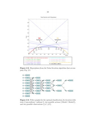
The pair of figures Fig. 2·2 and Fig. 2·3 demonstrate what a stereotypical POMDP
solution (for a toy problem) looks like. These figures describe the optimal set of solution
hyperplanes and the optimal policy for SM on a set of locations given a vector of prices
for resource costs (i.e. assuming for the moment that we already know what the optimal
resource prices are). The brown and magenta hyperplanes (nodes 2 and 6 w.r.t. Fig. 2·3
are very nearly parallel to the neighboring hyperplanes and therefore two of the three
hyperplanes with node id’s 1–3 are very nearly redundant (dominated) and the same
goes for node id’s 5–7. The smaller the extent of a hyperplane in the concave (for cost
functions) hull of the set of hyperplanes, the less role it has to play in the optimal
value function. In this example the cost of the ‘Mode1’ action was 0.1 units and that
of ‘Mode2’ was 0.18 units. If the ‘Mode2’ cost is changed to 0.2 units then there
are only 7 hyperplanes in the optimal set of hyperplanes (i.e. the value function) and
‘Mode2’ is not used at all. These results are relative to the prior probability and sensor
statistics. The alpha vectors (i.e. hyperplane coefficients) and actions associated with
each hyperplane (equivalently decision-tree node) can be seen in the inset below the
value function. The state enumeration was X={‘non-military’,‘military’}. The alpha](https://image.slidesharecdn.com/9f5467db-22a0-4b25-9f85-d66c2d62a6f8-160910233158/85/dissertation-43-320.jpg)
![22
vector coefficients give the classification + measurement cost of a location having each
one of these states w.r.t. this enumeration.
In Fig. 2·3, assume hypothesis ‘H2’ corresponds to ‘Declare military vehicle’ and
‘H1’ is the null hypothesis (‘Declare non-military vehicle’). In this policy the arrows
leaving each node on top represent observation ‘y1’ (‘non-military’), and the arrows on
bottom represent ‘y2’ (‘military’). The 9 nodes on the left of this policy correspond
to the 9 hyperplanes that make up Fig. 2·2. If there had been more than two possible
actions and two possible observations, then after a few stages there could easily have
been thousands of distinct nodes in the initial stage! This figure uses a model with a
dummy/terminal capture state, so it is possible to stop sensing at any time.
The use of two states, one sensor with two modes, two observations (the same type of
observations for both modes) for a horizon 5 (4 sensing actions+classification) POMDP
results in 9 hyperplanes based on the particular cost structure used: ‘Mode1’ costs
0.1 units and ‘Mode2’ costs 0.18 units. False alarms (FAs) and Missed detections (MDs)
each cost 1 unit. For problems with several sensors, 4 possible states and 3 modes
per sensor with 3 possible observations, there are frequently on the order of 500–1000
hyperplanes for a horizon 5 POMDP. Whereas originally this work was done using the
Witness Algorithm in a modified version of pomdp-solve-5.3 [Cassandra, 1999], this
algorithm is slow when solving 1000’s (later millions) of POMDPs in a loop. Therefore,
by default we use the Finite Grid algorithm (PBVI) within our customized version of
pomdp-solve-5.3 with 500–1000 belief-points to solve POMDPs. This allows a POMDP
of this size to be solved within about 0.2 sec on a single-core, Intel P4, 2.2 GHz, Linux
machine.
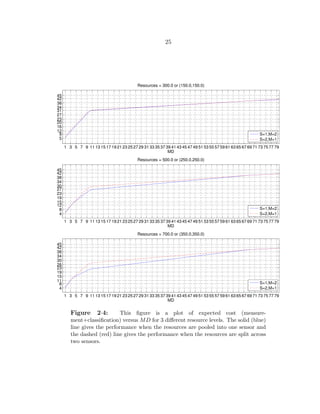
There is a trade-off between correctly detecting objects and engendering false alarms.
Fig. 2·4 illustrates how the overall classification cost increases as the ratio of the MD:FA
cost increases (from 1:1 through 80:1) for 3 resource levels {300, 500, 700} according to](https://image.slidesharecdn.com/9f5467db-22a0-4b25-9f85-d66c2d62a6f8-160910233158/85/dissertation-44-320.jpg)
![24
two cases: in the first case the resources are all available to a single sensor that supports
two modes of operation {‘mode1’, ‘mode2’}, and in the second case the resources are
equally divided between two identical sensors that each support the same two modes of
operation. Partitioning resources in this way adds an additional constraint that increases
classification cost. We also observe that the larger the quantity of resources available,
the larger the discrepancy between the S = 1, M = 2 case and the S = 2, Ms = 1 ∀ s
case.
In order to have meaningful POMDP solutions, we must have a way of coordinating
the sensing activities between various locations. Lagrange multipliers and Lagrangian
Relaxation provide this coordinating mechanism. Writing our policies for SM in terms
of mixed strategies allows linear programming techniques to be used for Lagrangian
Relaxation. To this end, we write Eq. 2.9 in terms of mixed strategies:
˜J∗
λ = min
γ∈Q(ΓL)
E
γ
N
i=1
c(xi, vi) +
T−1
t=0
S
s=1
λsrs(us(t)) −
S
s=1
λsRs (2.10)
where the strategy γ maps the current information state π(t) to the choice of us(t) ∀ s.
At stage T the strategy γ also determines the classification decisions vi ∀ i. On account
of the fact that we chose a relaxed form of resource constraint in Eq. 2.2, we know that
the actual optimal cost must be lower bounded by Eq. 2.10 because we have expanded
the space of feasible actions. This identification leads to the inequality:
J∗
≥ sup
λ1,...,λS≥0
˜J∗
λ1,...,λS
(2.11)
As shown in [Casta˜n´on, 2005a], Eq. 2.11 is the dual of the LP:
min
q∈Q(ΓL)
γ∈ΓL
q(γ) E
γ
[J(γ)] (2.12)](https://image.slidesharecdn.com/9f5467db-22a0-4b25-9f85-d66c2d62a6f8-160910233158/85/dissertation-46-320.jpg)
![26
γ∈ΓL
q(γ) E
γ
N
i=1
T−1
t=0
rs(us(t)) ≤ Rs ∀ s ∈ [1, . . . , S] (2.13)
γ∈ΓL
q(γ) = 1 (2.14)
where we have one constraint for each of the S sensor resource pools and an additional
simplex constraint in Eq. 2.14 which ensures that q ∈ Q(ΓL) forms a valid probability
distribution.
This is a large LP, where the number of possible variables are the strategies in
ΓL. However, the total number of constraints is S + 1, which establishes that optimal
solutions of this LP are mixtures of no more than S + 1 strategies. Thus, one can use a
Column Generation approach [Gilmore and Gomory, 1961,Dantzig and Wolfe, 1961,Yost
and Washburn, 2000] to quickly identify an optimal mixed strategy that solves the relaxed
(i.e. approximate) form of our SM problem. (See Appendix A.3 for an overview of
Column Generation). To use Column Generation with the LP formulation Eq. 2.12 -
Eq. 2.14, we break the original problem hierarchically into two new sets of problems
that are called the master problem and subproblems. There is one POMDP subproblem
for each location. The master problem consists of identifying the appropriate values of
the Lagrange multipliers, λs ∀ s, to determine how resources should be shared across
locations, and the subproblems consist of using these Lagrange multipliers to compute
the expected resource usage and expected classification cost for each of the N locations.
See Fig. 2·5 for a pictorial representation.
Column Generation works by solving Eq. 2.12 and Eq. 2.13, restricting the mixed
strategies to be mixtures of a small subset Γ′
L ⊂ ΓL. The solution of the restricted LP
has optimal dual prices λs, s = 1, . . . , S. Using these prices, one can determine a corre-
sponding optimal pure strategy by minimizing Eq. 2.9, which the results in [Casta˜n´on,
2005b] show can be decoupled into N independent optimization problems, one for each
location. Each of the subproblems is solved as a POMDP using standard algorithms,](https://image.slidesharecdn.com/9f5467db-22a0-4b25-9f85-d66c2d62a6f8-160910233158/85/dissertation-48-320.jpg)
![27
Figure 2·5: Schematic showing how the master problem coordinates the ac-
tivities of the POMDP subproblems using Column Generation and Lagrangian
Relaxation. After the master problem generates enough columns to find the
optimal values for the Lagrange multipliers, there is no longer any benefit to
violating one of the resource constraints and the subproblems (with augmented
costs) are decoupled in expectation.
such as Point-Based Value Iteration (PBVI), Appendix A.2 [Pineau et al., 2003], to de-
termine the best pure strategy γ1 for these prices. Solving all of the subproblems allows a
new column to be generated by providing values for the expected classification cost and
expected resource utilization for a given set of sensor prices λs; these values become the
coefficients in the new column in the (Revised) Simplex Tableau of the master problem.
The column that is generated will be a pure strategy that is not already in the basis of
the LP (or else the master problem would have converged). If the best pure strategy, γ1,
for the prices, λs ∀ s ∈ [1, . . . , S], is already in the set Γ′
L, then the solution of Eq. 2.12
and Eq. 2.13 restricted to Q(Γ′
L) is an optimal mixed strategy over all of Q(ΓL), and
the Column Generation algorithm terminates. Otherwise, the strategy γ1 is added to
the admissible set Γ′
L, and the iteration is repeated. The solution to this algorithm is
a set of mixed strategies that achieve a performance level that is a lower bound on the
original SM optimization problem with hard constraints.
2.2.2 Addressing the Search versus Exploitation Trade-off
As one contribution of this dissertation, we address how to non-myopically trade-off be-
tween spending time searching for objects versus spending time acting on them. This is](https://image.slidesharecdn.com/9f5467db-22a0-4b25-9f85-d66c2d62a6f8-160910233158/85/dissertation-49-320.jpg)
![28
P(y1,1(t)|xi, u1(t)) = P(y1,2(t)|xi, u2(t)) = P(y1,3(t)|xi, u3(t)) =
empty
car
truck
SAM
0
B
B
B
B
B
@
0.92 0.04 0.04
0.08 0.46 0.46
0.08 0.46 0.46
0.08 0.46 0.46
1
C
C
C
C
C
A
o1 o2 o3
0
B
B
B
B
B
@
0.95 0.03 0.02
0.05 0.85 0.10
0.05 0.10 0.85
0.05 0.10 0.85
1
C
C
C
C
C
A
o1 o2 o3
0
B
B
B
B
B
@
0.97 0.02 0.01
0.02 0.95 0.03
0.02 0.90 0.08
0.02 0.03 0.95
1
C
C
C
C
C
A
o1 o2 o3
Table 2.1: Example of expanded sensor model for an SEAD mission
scenario where the states are {‘empty’, ‘car’, ‘truck’, ‘SAM’} and the
observations are ys,m = {o1 = ‘see nothing’, o2 = ‘civilian vehicle’, o3
= ‘military vehicle’} ∀ s, m. This setup models a single sensor with
modes {u1 = ‘search’, u2 = ‘mode1’, u3 = ‘mode2’} where mode2 by
definition is a higher-quality mode than mode1. Using mode1, trucks can
look like SAMs, but cars do not look like SAMs.
an easy generalization to make: object confusion matrices can be used to allow inferenc-
ing based on detection only. To accomplish this, we augment the sensor model used in
example of [Casta˜n´on, 2005a] with a ‘search’ action that supports a low-res mode of op-
eration (with low resource demand) designed for object detection but incapable of object
classification. Our sensor observation models can be made non-informative w.r.t. object
type by setting the conditional probability of an observation for each type of object to be
the same as in Table 2.1. As a simple starting point for the new sensor model, we consider
three possible values of observations : {o1 = ‘see nothing’, o2 = ‘uninteresting object’,
o3 = ‘interesting object’} that have known statistics and are the result of pre-processing
and thresholding sensor data. The ‘search’ action effectively returns the joint probability
of P(o2 ∩ o3|xi, u1).
2.2.3 Tracing Decision-Trees
One hindrance is that the hyperplanes given by a POMDP solver that represent the
expected cost-to-go are in terms of total cost. In order to create a new column, it is
necessary to separate out the classification cost from the measurement costs. This pro-
cess is best illustrated with an example. Consider Fig. 2·6. This figure is an illustration](https://image.slidesharecdn.com/9f5467db-22a0-4b25-9f85-d66c2d62a6f8-160910233158/85/dissertation-50-320.jpg)
![29
of “tracing” or “walking” a POMDP decision-tree solution to calculate expected clas-
sification costs and resource utilizations for a subproblem. The states in this example
are indexed as {‘military’, ‘truck’, ‘car’, ‘empty’}. The dot-product of the probability
vector for the current information state, in this example π(0) = [0.02 0.06 0.12 0.80]T
,
with the best hyperplane returned by Value Iteration (or the approximation PBVI)
gives the total cost for location i: Ji,total = Ji,measure +Ji,classify, from which we can calcu-
late the subproblem classification cost, Ji,classify, once we subtract out its measurement
cost, Ji,measure. To subtract out the measurement cost, we must recursively traverse the
decision-tree and sum up the (expected) cost of each potential measurement action. The
probability mixture weights in the expected cost of each action are given by the obser-
vation probabilities P(ys,m(t)|πi(t), u(t)), where u(t) is the sensor action taken. For the
particular initial probability of π(0), only actions in the set {‘wait’, ‘search’} are part
of the optimal solution (for simplicity of illustration). The numbers in blue represent
the conditional likelihood of an observation occurring, and the color of each node rep-
resents the optimal choice of action for that information state (and nearby information
states): {white=‘wait’, aqua=‘search’}. Given this decision-tree that represents the op-
timal course of action for the information state π(0), the set of possible future beliefs
and the relative likelihood of each belief occurring are shown. The possible beliefs and
likelihoods display their respective observation histories up to time t using the conven-
tion o = {y(0), . . . , y(t−1)}. In this example false alarm and missed detection costs are
equal (FA=MD), and the (time-invariant) likelihoods for the ‘search’ action are:
P(ysearch(t)|xi, ‘search’) =
0.08 0.46 0.46
0.08 0.46 0.46
0.08 0.46 0.46
0.92 0.04 0.04
In this matrix, the states xi vary along the rows, and the observations {‘o0’, ‘o1’, ‘o2’} (for
{‘see nothing’, ‘see non-military vehicle’, ‘see military vehicle’}) vary across the columns.](https://image.slidesharecdn.com/9f5467db-22a0-4b25-9f85-d66c2d62a6f8-160910233158/85/dissertation-51-320.jpg)
![30
All indices are 0-based. There were 3 observations (which in general implies three child
nodes for every node in the decision-tree) for some actions, but the search action has a
uniform observation probability over all non-empty observations (all observations except
‘o0’), and therefore the latter two future node indices for search nodes (nodes that specify
search actions) are always the same. (This keeps the example tractable). For a ‘wait’
action, all three future nodes are the same because there is only one possible future belief-
state. The green terminal classification (‘declaration’) node represents the decision that
a location contains a benign object (‘truck’, ‘car’) and the gray declaration node that the
location is ‘empty’. The nodes are labeled using the scheme: ‘[nodeId nextNodeId[o0]
nextNodeId[o1] nextNodeId[o2]’, so for the root node (stage 0, node 0) the next node will
be (stage 1, node 4) if the observation is o0, (stage 1, node 1) if the observation is o1, and
again (stage 1, node 1) for observation o2 because a search action can not discriminate
object type. The declaration nodes have no future nodes, which is indicated with ‘X’
characters. Notice there are two possible information states (beliefs) for π(2) at nodeId 0
during the second-to-last stage, and therefore the conditional observation probabilities
at this node are path-dependent (the nodes represent a convex region of belief-space,
they do not represent a unique probability vector). The red star and black box in the
figure indicate the two different possible beliefs (and therefore the two different possible
sets of observation likelihoods) for this node. The vector πnew(1) represents the future
belief-state after one time interval if no action is taken. In other words the state is
non-stationary in this example and in fact a HMM model was imposed on the state of
each location. The HMM has an arrival probability (chance of leaving the ‘empty’ state)
at each stage of 5%: the probability of a location being empty goes from 80% to 76% in
one stage (0.05 × 0.80 = 0.76), and this probability mass diffuses elsewhere (increases
the chance of state ‘military’).
One caveat w.r.t. the software package we used (an extensively modified version of](https://image.slidesharecdn.com/9f5467db-22a0-4b25-9f85-d66c2d62a6f8-160910233158/85/dissertation-52-320.jpg)
![31
Tony Cassandra’s pomdp-solve-5.3 [Cassandra, 1999]) that comes into play with a time-
varying state is that an observation at stage t (undesirably) refers to the system state
at time t+1. This is the convention used in the robotics community but is not desirable
in an SM context: it’s anti-causal. There is no difference if the state is stationary. We
will pick up this topic of non-stationarity again in the next section and then as one of
the main topics of Ch. 4.
Each possible terminal belief-state is indicated along with the associated proba-
bility of classification error in the lower-right corner. By way of example, while the
P(error|π(3;o=0,0,0)) = 0.0052, the expected contribution of this error to the terminal
classification cost is even smaller because the likelihood of this particular outcome is
the joint probability of the associated observations: P(y0 = 0, y1 = 0, y2 = 0) = P(y0 =
0)P(y1 = 0)P(y2 = 0) = 0.7184∗0.8567∗0.8724 (the numbers in blue along this realiza-
tion of the decision-tree). The variables in the conditioning were suppressed for brevity.
Unfortunately, walking the decision-trees to back out classification costs is rather slow
(recursive function calls) with large trees, requiring on the order of 15% of the compu-
tational time in simulations with horizon 6 plans (PBVI took around 80%), however at
least this operation is parallelizable, and the PBVI algorithm is parallelizable as well!
As a slightly more complex example of a set of POMDP solutions and what tracing
decision-trees entails, consider Fig. 2·7 and Fig. 2·8 which show a pair of decision-trees
for a horizon 6 scenario with D = 3 and Ms = 3 (plus a ‘wait’ action). The state
‘empty’ has been added to X and a ‘search’ mode has been added to the action space.
The ‘search’ mode is able to quickly detect the presence or absence of an object but
completely unable to specify object type. In addition, an HMM has been used instead
of having the state be stationary such that the model allows for a non-zero probability
of object arrivals from one stage to the next. This example uses an object arrival
probability of 5% / stage. It is interesting to note the situations in which the optimal](https://image.slidesharecdn.com/9f5467db-22a0-4b25-9f85-d66c2d62a6f8-160910233158/85/dissertation-53-320.jpg)
![33
Figure 2·7: Strategy 1 (mixture weight=0.726). πi(0) = [0.1 0.6 0.2 0.1]’
∀ i ∈ [0, . . . , 9], πi(0) = [0.80 0.12 0.06 0.02]T
∀ i ∈ [10, . . . , 99]. The first 10
objects start with node 5, the remaining 90 start with node 43. The notation
[i Ni0 Ni1 Ni2] indicates the next node/action from node i as a function of
observing the 0th, 1st or 2nd observations respectively.
strategy is to wait to act versus to gain as much information as possible with the time
available.
2.2.4 Violation of Stationarity Assumptions
At first glance, using a HMM state model with arrival probabilities, as in Fig. 2·6,
seems to violate our stationarity assumptions that allowed us to decompose the original
problem into one in which we have parallel virtual time-lines happening at each location
and where we did not need to worry about the sequencing of events between these
locations. Given stationarity, the order in which locations are sensed does not matter.
We notice that the same thing is true for a HMM with arrival probabilities because
having an object arrive at a location does not influence the optimal choice of sensing](https://image.slidesharecdn.com/9f5467db-22a0-4b25-9f85-d66c2d62a6f8-160910233158/85/dissertation-55-320.jpg)
![34
Figure 2·8: Strategy 2 (mixture weight=0.274) πi(0) = [0.1 0.6 0.2 0.1]’ ∀ i ∈
[0, . . . , 9], πi(0) = [0.80 0.12 0.06 0.02]T
∀ i ∈ [10, . . . , 99]. The first 10 objects
start with node 6, the remaining 90 start with node 18.
actions at that location in the past when the location was empty. If a location is
empty, there is no sensing to be done. An arrival only affects the best choices of sensing
action for that location in the future, and we replan every round. Therefore we can
still decouple sensing actions across locations when we have arrivals. The problem in
developing a model for a time-varying state is how to handle object departures. If an
object departs (a location becomes empty), now the best choice of previous actions for
that location are affected retroactively.
2.3 Column Generation And POMDP Subproblem Example
In this section we present an example of the Column Generation algorithm and POMDP
algorithms discussed previously. In this simple example we consider 100 objects (N=100),
2 possible object types (D=2) with X = {‘non-military vehicle’, ‘military vehicle’}, and](https://image.slidesharecdn.com/9f5467db-22a0-4b25-9f85-d66c2d62a6f8-160910233158/85/dissertation-56-320.jpg)
![35
2 sensors that each have one mode (S = 2 and Ms = 1 ∀ s ∈ {1, 2}). Sensor s actions
have resource costs: rs, where r1 = 1, r2 = 2. Sensors return 2 possible observation
values, corresponding to binary object classifications, with likelihoods:
P(y1,1(t)|xi, u1(t)) P(y2,1(t)|xi, u2(t))
0.90 0.10
0.10 0.90
0.92 0.08
0.08 0.92
where the (j, k) matrix entry denotes the likelihood that y = k if xi = j. The second
sensor has 2% better performance than the first sensor but requires twice as many
resources to use. Each sensor has Rs = 100 units of resources, and can view each
location. Each of the 100 locations has a uniform prior of πi = [0.5 0.5]T
∀ i. For the
performance objective, we use c(xi, vi) = 1 if xi = vi, and 0 otherwise, so the cost is
1 unit for a classification error.
Table 2.2 demonstrates the Column Generation solution process. The first three
columns are initialized by guessing values of resource prices and obtaining the POMDP
solutions, yielding expected costs and expected resource use for each sensor at those
resource prices. A small LP is solved to obtain the optimal mixture of the first three
strategies γ1, . . . , γ3, and a corresponding set of dual prices. These dual prices are used
in the POMDP solver to generate the fourth column γ4, which yields a strategy that is
different from that of the first 3 columns. The LP is re-solved for mixtures of the first
4 strategies, yielding new resource prices that are used to generate the next column. This
process continues until the solution using the prices after 7 columns yields a strategy
that was already represented in a previous column, terminating the algorithm. The
optimal mixture combines the strategies of the second, fifth and sixth columns. When
the master problem converges, the optimal cost, J∗
, for the mixed strategy is 5.95 units.
The resulting decision-trees are illustrated in Fig. 2·9, where branches up indicate
measurements y = 1 (‘non-military’) and down y = 2 (‘military’). The red and green](https://image.slidesharecdn.com/9f5467db-22a0-4b25-9f85-d66c2d62a6f8-160910233158/85/dissertation-57-320.jpg)


![41
• str1: Select the pure strategy with maximum probability.
• str2: Randomly select a pure strategy per location according to the optimal mix-
ture probabilities.
• str3: Select the pure strategy with positive probability that minimizes the expected
sensor resource use over all sensors (and leaves resources for use in future stages).
The column gen simulator that we have developed also supports two other methods
for converting mixed strategies to sensing actions:
• str4: Select the pure strategy that minimizes classification cost.
• str5: Randomly select a single pure strategy for all locations jointly according to
the optimal mixture probabilities.
However these latter two methods for RH control were deemed to be less useful and
therefore were not included in the fractional factorial design of experiments analysis.
The pure strategies that are selected for each location map the current information
sets, Ii(t) for location i, into a deterministic sensing action. ‘str1’ and ‘str3’ choose
the same pure strategy to use across all locations, but ‘str2’ chooses a pure strategy
on a location-by-location basis. Note that there may not be enough sensor resources
to execute the selected actions, particularly in the case where the pure strategy with
maximum probability is selected. To address this, we rank sensing actions by their
expected entropy gain [Kastella, 1996]:
Gain(us(t)) =
H(πi(t)) − Ey[H(πi(t + 1))|y, us(t)]
rs(us(t))
(3.1)
where Ey[] is the expected future entropy value. We schedule sensor actions in order
of decreasing expected entropy gain, and perform those actions at stage t that have
enough sensor resources to be feasible. We also use the Entropy Gain algorithm at the](https://image.slidesharecdn.com/9f5467db-22a0-4b25-9f85-d66c2d62a6f8-160910233158/85/dissertation-63-320.jpg)
![42
very end of a simulation when resources are nearly depleted, and the higher cost sensor
modes are no longer feasible, see Appendix B for more information. (When the horizon
is very short, the Entropy Gain algorithm is nearly-optimal, so this does not constitute
a significant performance limitation in our design).
The measurements collected from the scheduled actions are used to update the infor-
mation states πi(t + 1) using Eq. 2.3. The resources used by the actions are eliminated
from the available resources to compute Rs(t + 1) using Eq. 2.4. The RH algorithm
is then executed from the new information state/resource state condition in iterative
fashion until all resources are expended.
3.2 Simulation Results
In order to evaluate the relative performance of the alternative RH algorithms, we
performed a set of simulations. In these experiments, there were 100 locations, each of
which could be empty, or have objects of three types, so the possible states of location i
were xi ∈ {0, 1, 2, 3} where type 1 represents cars, type 2 trucks, and type 3 military
vehicles. Sensors can have several modes: a ‘search’ mode, a low resolution ‘mode1’ and
a high resolution ‘mode2’. The search mode primarily detects the presence of objects;
the low resolution mode can identify cars, but confuses the other two types, whereas the
high resolution mode can separate the three types. Observations are modeled as having
three possible values. The search mode consumes 0.25 units of resources, whereas the
low-resolution mode consumes 1 unit and the high resolution mode 5 units, uniformly
for each sensor and location. Table 3.1 shows the likelihood functions that were used in
the simulations.
Initially, each location has a state with one of two prior probability distributions:
πi(0) = [0.10 0.60 0.20 0.10]T
, i ∈ [1, . . . , 10] or πi(0) = [0.80 0.12 0.06 0.02]T
, i ∈
[11, . . . , 100]. Thus, the first 10 locations are likely to contain objects, whereas the other](https://image.slidesharecdn.com/9f5467db-22a0-4b25-9f85-d66c2d62a6f8-160910233158/85/dissertation-64-320.jpg)
![45
plan is accounting for, — after doing multiple planning iterations. (A simulation may
re-plan 5+ times before resources are exhausted, but the bound was computed assuming
there will only be a maximum of two sensing opportunities per object for a horizon=3
problem). Obviously, the easily classified objects are ruled out of the competition for
sensor resources (their identities are decided upon) early in the simulation process,
and with every additional planning iteration, sensor resources are concentrated on the
remaining objects whose identities are uncertain. In this situation the approximate
sensor plan from the Column Generation algorithm does not match well with the way
events unfold, and the “bound” is not a bound. However, after choosing a horizon that
accounts appropriately for how many RH planning iterations there will be and how
many sensing opportunities will take place at each location, the bounds are tight.
In terms of which strategy is preferable for converting the mixed strategies to a pure
strategy, the results of Table 3.3 are unclear. For short planning horizons in the RH
algorithms, the preferred strategy appears to be to use the least resources (str3): because
planning with a longer horizon improves performance minimally, we find that using a RH
replanning approach with a short horizon in conjunction with a resource-conservative
planning strategy can be used to reduce computation time with limited performance
degradation. For the longer horizons, there was no significant difference in performance
among the three strategies we investigated.
In the next set of experiments, we compare the use of heterogeneous sensors that
have different modes available. In these experiments, the 100 locations are guaranteed
to have an object, so xi = 0 is not feasible. The prior probability of object type for
each location is πi(0) = [0 0.7 0.2 0.1]T
. Table 3.5 shows the results of experiments with
sensors that have all sensing modes, versus an experiment where one sensor has only
a low-resolution mode and the other sensor has both high and low-resolution modes.
The table shows the lower bounds predicted by the Column Generation algorithm, to](https://image.slidesharecdn.com/9f5467db-22a0-4b25-9f85-d66c2d62a6f8-160910233158/85/dissertation-67-320.jpg)
![46
MD = 1 MD = 5 MD = 10
Hor. 3 str1 str2 str3 str1 str2 str3 str1 str2 str3
Res 30 3.64 3.85 3.85 11.82 12.88 12.23 15.28 14.57 14.50
Res 50 2.40 2.80 2.43 6.97 6.93 7.84 10.98 9.99 10.45
Res 70 2.45 2.32 1.88 3.44 3.99 4.04 6.14 6.48 5.10
Hor. 4
Res 30 3.58 3.46 3.52 12.28 12.62 11.90 14.48 15.91 15.59
Res 50 2.37 2.21 2.33 7.44 7.44 7.20 9.94 9.28 10.65
Res 70 1.68 1.33 1.60 3.59 3.57 3.62 6.30 5.18 5.86
Hor. 6
Res 30 3.51 3.44 3.73 11.17 11.85 12.09 15.17 14.99 13.6
Res 50 2.28 2.11 2.31 7.29 8.02 7.70 10.67 10.47 11.25
Res 70 1.43 1.38 1.44 3.60 3.73 3.84 4.91 5.09 5.94
Table 3.3: Simulation results for 2 homogeneous, multi-modal sensors in
a search and classify scenario. str1: select the most likely pure strategy for
all locations; str2: randomize the choice of strategy per location according to
mixture probabilities; str3: select the strategy that yields the least expected
use of resources for all locations. See Fig. 3·2 - Fig. 3·4 for the graphical version
of this table.
MD
Horizon 3 1 5 10
Res[30, 30] 4.96 12.11 14.64
Res[50, 50] 4.09 8.79 11.16
Res[70, 70] 3.38 6.20 8.19
Horizon 4
Res[30, 30] 4.24 11.86 14.56
Res[50, 50] 3.09 6.72 9.50
Res[70, 70] 2.16 4.24 5.94
Horizon 6
Res[30, 30] 3.35 11.50 13.85
Res[50, 50] 2.21 6.27 9.40
Res[70, 70] 1.32 2.95 4.96
Table 3.4: Bounds for the simulations results in Table 3.3. When the horizon
is short, the 3 MPC algorithms execute more observations per object than were
used to compute the “bound”, and therefore, in this case, the bounds do not
match the simulations; otherwise, the bounds are good.](https://image.slidesharecdn.com/9f5467db-22a0-4b25-9f85-d66c2d62a6f8-160910233158/85/dissertation-68-320.jpg)
![47
1 2 3
0
5
10
15
FA:MD = 1 Bound = 4.960
E[J]
1 2 3
0
5
10
15
FA:MD = 5 Bound = 12.110
E[J]
1 2 3
0
5
10
15
FA:MD = 10 Bound = 14.640
E[J]
1 2 3
0
5
10
15
FA:MD = 1 Bound = 4.090
E[J]
1 2 3
0
5
10
15
FA:MD = 5 Bound = 8.790
E[J]
1 2 3
0
5
10
15
FA:MD = 10 Bound = 11.160
E[J]
1 2 3
0
5
10
15
FA:MD = 1 Bound = 3.380
E[J]
1 2 3
0
5
10
15
FA:MD = 5 Bound = 6.200
E[J]
1 2 3
0
5
10
15
FA:MD = 10 Bound = 8.190
E[J]
Horizon = 3
Resources =
60.0
Resources =
100.0
Resources =
140.0
Figure 3·2: This figure is the graphical version of Table 3.3 for horizon 3.
Simulation results for two sensors with full visibility and detection (X=’empty’,
’car’, ’truck’, ’military’) using πi(0) = [0.1 0.6 0.2 0.1]T
∀ i ∈ [0..9], πi(0) =
[0.80 0.12 0.06 0.02]T
∀ i ∈ [10..99]. There is one bar in each sub-graph for
each of the three simulation modes studied in this chapter. The theoretical
lower bound can be seen in the upper-right corner of each bar-chart.
1 2 3
0
5
10
15
FA:MD = 1 Bound = 4.240
E[J]
1 2 3
0
5
10
15
FA:MD = 5 Bound = 11.860
E[J]
1 2 3
0
5
10
15
FA:MD = 10 Bound = 14.560
E[J]
1 2 3
0
5
10
15
FA:MD = 1 Bound = 3.090
E[J]
1 2 3
0
5
10
15
FA:MD = 5 Bound = 6.720
E[J]
1 2 3
0
5
10
15
FA:MD = 10 Bound = 9.500
E[J]
1 2 3
0
5
10
15
FA:MD = 1 Bound = 2.160
E[J]
1 2 3
0
5
10
15
FA:MD = 5 Bound = 4.240
E[J]
1 2 3
0
5
10
15
FA:MD = 10 Bound = 5.940
E[J]
Horizon = 4
Resources =
60.0
Resources =
100.0
Resources =
140.0
Figure 3·3: This figure is the graphical version of Table 3.3 for horizon 4.](https://image.slidesharecdn.com/9f5467db-22a0-4b25-9f85-d66c2d62a6f8-160910233158/85/dissertation-69-320.jpg)
![48
1 2 3
0
5
10
15
FA:MD = 1 Bound = 3.350
E[J]
1 2 3
0
5
10
15
FA:MD = 5 Bound = 11.500
E[J]
1 2 3
0
5
10
15
FA:MD = 10 Bound = 13.850
E[J]
1 2 3
0
5
10
15
FA:MD = 1 Bound = 2.210
E[J]
1 2 3
0
5
10
15
FA:MD = 5 Bound = 6.270
E[J]
1 2 3
0
5
10
15
FA:MD = 10 Bound = 9.400
E[J]
1 2 3
0
5
10
15
FA:MD = 1 Bound = 1.320
E[J]
1 2 3
0
5
10
15
FA:MD = 5 Bound = 2.950
E[J]
1 2 3
0
5
10
15
FA:MD = 10 Bound = 4.960
E[J]
Horizon = 6
Resources =
60.0
Resources =
100.0
Resources =
140.0
Figure 3·4: This figure is the graphical version of Table 3.3 for horizon 6.
illustrate the change in performance expected from the different architectural choices
of sensors. The results indicate that specialization of one sensor can lead to significant
degradation in performance due to inefficient use of its resources.
The next set of results explore the effect of spatial distribution of sensors. We con-
sider experiments where there are two homogeneous sensors which have only partially-
overlapping coverage zones. (We define a “visibility group” as a set of sensors that have
a common coverage zone). Table 3.6 gives bounds for different percentages of overlap.
Note that, even when there is only 20% overlap, the achievable performance is similar to
that of the 100% overlap case in Table 3.5, indicating that proper choice of strategies can
lead to efficient sharing of resources from different sensors by equalizing their workload.
The last set of simulation results we consider show the performance of these RH
algorithms for three homogeneous sensors with partial sensor overlap, no detection and
varying resource levels. The visibility groups are graphically portrayed in Fig. 3·5.
Table 3.7 presents the simulated cost values averaged over 100 simulations of the three
different RH algorithms. See Table 3.8 for the accompanying lower bounds. Fig. 3·6 -
Fig. 3·8 display the graphical version of these tables. The results support our previous](https://image.slidesharecdn.com/9f5467db-22a0-4b25-9f85-d66c2d62a6f8-160910233158/85/dissertation-70-320.jpg)
![49
Homogeneous Heterogeneous
MD MD
Horizon 3 1 5 10 1 5 10
Res[150, 150] 5.689 16.928 30.380 6.338 18.150 31.233
Res[250, 250] 4.614 16.114 25.917 5.527 16.767 29.322
Res[350, 350] 4.225 15.301 21.453 5.123 16.414 27.411
Horizon 4
Res[150, 150] 5.016 16.059 20.606 5.641 16.849 20.606
Res[250, 250] 3.939 9.461 12.662 4.576 12.047 14.873
Res[350, 350] 3.352 8.578 12.474 4.275 9.407 12.651
Horizon 6
Res[150, 150] 4.618 15.661 19.564 5.271 16.202 19.564
Res[250, 250] 2.919 8.237 10.913 3.321 8.830 11.347
Res[350, 350] 2.175 4.860 7.151 2.658 6.629 9.174
Table 3.5: Comparison of lower bounds for 2 homogeneous, bi-modal sensors
(left 3 columns) versus 2 heterogeneous sensors in which S1 has only ‘mode1’
available but S2 supports both ‘mode1’ and ‘mode2’ (right 3 columns). There
is 1 visibility-group with πi(0) = [0.7 0.2 0.1]T
∀ i ∈ [0..99]. For many of the
cases studied there is a performance hit of 10–20%.
Overlap 60% Overlap 20%
MD MD
Horizon 3 1 5 10 1 5 10
Res[150, 150] 5.69 16.93 30.38 5.69 16.93 30.38
Res[150, 150] 4.61 16.11 25.98 4.61 16.11 25.92
Res[150, 150] 4.23 15.30 21.45 4.23 15.30 21.45
Horizon 4
Res[150, 150] 5.02 16.06 20.61 5.02 15.93 20.61
Res[150, 150] 3.94 9.46 12.66 3.94 9.46 12.66
Res[150, 150] 3.35 8.58 12.47 3.35 8.58 12.47
Horizon 6
Res[150, 150] 4.62 15.66 19.56 4.62 15.66 19.56
Res[150, 150] 2.92 8.25 10.91 2.94 8.24 10.91
Res[150, 150] 2.18 4.86 7.19 2.18 4.86 7.16
Table 3.6: Comparison of sensor overlap bounds with 2 homogeneous, bi-
modal, sensors and 3 visibility-groups. Both configurations use the prior πi(0) =
[0.7 0.2 0.1]T
. Compare and contrast with the left half of Table 3.5, most of
the time the two sensors have enough objects in view to be able to efficiently
use their resources for both the 60% and 20% overlap configurations; only the
bold numbers are different.](https://image.slidesharecdn.com/9f5467db-22a0-4b25-9f85-d66c2d62a6f8-160910233158/85/dissertation-71-320.jpg)
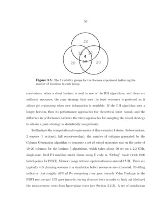
![51
MD = 1 MD = 5 MD = 10
Hor. 3 str1 str2 str3 str1 str2 str3 str1 str2 str3
Res 100 5.26 6.08 5.57 17.23 17.44 16.79 22.02 21.93 22.16
Res 166 5.91 4.81 3.13 10.23 11.91 9.21 14.19 16.66 12.85
Res 233 3.30 3.75 3.43 10.15 9.32 5.88 14.49 12.55 8.21
Hor. 4
Res 100 5.32 5.58 5.93 17.26 16.88 16.17 21.92 20.94 21.35
Res 166 3.42 4.07 3.24 8.63 8.00 9.04 12.05 11.71 14.08
Res 233 3.65 3.07 3.29 5.27 7.14 5.38 8.25 10.08 7.90
Hor. 6
Res 100 5.79 5.51 5.98 17.13 17.90 17.44 22.03 20.56 22.17
Res 166 2.96 2.68 2.72 10.22 8.33 9.08 9.82 11.47 11.57
Res 233 1.52 2.00 1.70 4.81 4.13 4.24 5.64 7.20 5.11
Table 3.7: Simulation results for 3 homogeneous sensors without using de-
tection but with partial overlap as shown in Fig. 3·5. See Fig. 3·6 - Fig. 3·8 for
the graphical version.
MD
Horizon 3 1 5 10
Res[30, 30] 5.69 16.93 30.38
Res[50, 50] 4.61 16.11 25.89
Res[70, 70] 4.26 15.31 21.48
Horizon 4
Res[30, 30] 5.02 15.92 20.61
Res[50, 50] 3.94 9.46 12.66
Res[70, 70] 3.35 8.58 12.48
Horizon 6
Res[30, 30] 4.62 15.66 19.56
Res[50, 50] 2.92 8.22 10.89
Res[70, 70] 2.18 4.87 7.18
Table 3.8: Bounds for the simulations results in Table 3.7. When the horizon
is short, the 3 MPC algorithms execute more observations per object than were
used to compute the bound, and therefore, in this case, the bounds do not
match the simulations; otherwise, the bounds are good.](https://image.slidesharecdn.com/9f5467db-22a0-4b25-9f85-d66c2d62a6f8-160910233158/85/dissertation-73-320.jpg)
![52
Figure 3·6: This figure is the graphical version of Table 3.7 for horizon 3.
Situation with no detection but limited visibility (X=’car’, ’truck’, ’military’)
using πi(0) = [0.70 0.20 0.10]T
∀ i ∈ [0..99]. There were 7 visibility-groups:
20x001, 20x010, 20x100, 12x011, 12x101, 12x110, 4x111. The 3 bars in each
sub-graph are for ‘str1’, ‘str2’, ‘str3’ respectively. The theoretical lower bound
can be seen in the upper-right corner of each bar-chart.
Figure 3·7: This figure is the graphical version of Table 3.7 for horizon 4.](https://image.slidesharecdn.com/9f5467db-22a0-4b25-9f85-d66c2d62a6f8-160910233158/85/dissertation-74-320.jpg)
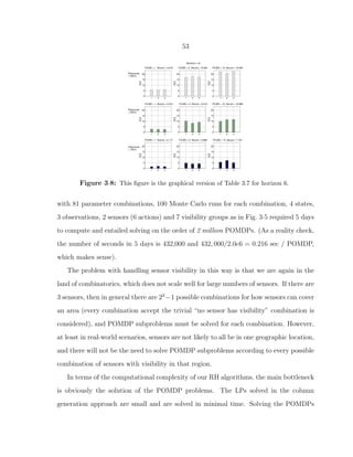

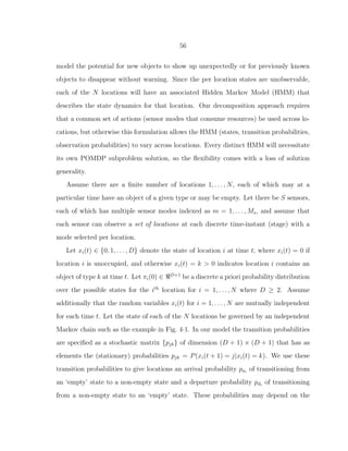
![58
time have elapsed. The action space for each stage is then the Cartesian product of
the set of feasible sensor-mode assignments for the N locations with the set of tentative
classification decisions for the N locations.
A sensor action by sensor s at stage t is the set of pairs:
us(t) = {(is(t), ms(t)) | is(t) ∈ Os(t), ms(t) ∈ Ms} (4.1)
where each pair consists of a location to observe is(t), and a sensor mode (independent
for each location) used to observe this location, ms(t), where the mode is restricted to
the set of feasible modes given the resource levels for each sensor. We assume that no two
sensors observe the same location at the same time in order to minimize the complexity
of the associated action and observation spaces. Let ui,s(t) refer to the sensor action
taken on location i with sensor s at stage t if any, or let ui,s(t) = ∅ otherwise.
Sensor measurements are modeled as belonging to a finite set ys,m ∈ {1, . . . , Ls}. The
likelihood of the measured value is assumed to depend on the sensor s, sensor mode m,
location i and on the true state at the location, xi(t), but not on the states of other loca-
tions (statistical independence). Denote this likelihood as P(ys,m(t)|xi(t), i, s, m). Thus,
the Markov models are observed through noisy measurements, resulting in HMMs. We
assume that this likelihood given xi(t) is time-invariant, and that the random measure-
ments ys,m(t) are conditionally independent of other measurements yσ,n(τ) given the
states xi(t), xj(τ) for all sensors s, σ and modes m, n provided i = j or τ = t.
Assume each sensor has a quantity Rs of resources available for measurements during
each stage, so there is a periodic constraint on sensor utilization. Associated with the
use of mode m by sensor s on location i at time t is a resource cost rs(ui,s(t)) to use this
mode, representing power or some other type of resource required to operate the sensor:
i∈Os(t)
rs(ui,s(t)) ≤ Rs ∀ s ∈ [1 . . . S]; ∀ t ∈ [1 . . . T] (4.2)](https://image.slidesharecdn.com/9f5467db-22a0-4b25-9f85-d66c2d62a6f8-160910233158/85/dissertation-80-320.jpg)
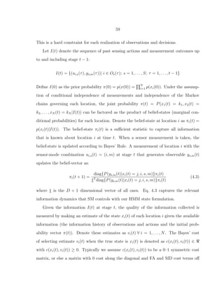
![60
the diagonal in the appropriate locations (relative to which state is not to be missed
and which state is a nuisance-detection).
The objective of this problem is to estimate the state of each location at each time
with minimum error as measured by the number of FAs and MDs:
J = min
γ∈Γ
E
γ
N
i=1
T
t=1
c(xi(t), vi(t)) (4.4)
subject to Eq. 4.2. The minimization is done over the (countable) space of admissible,
adaptive feedback strategies γ ∈ Γ. In this context, a strategy γ is a time-varying
mapping from an information set (history) to a sensor action and tentative classification
decision.
After replacing the hard resource constraint in Eq. 4.2 with an expected-resource-use
constraint for each of the S sensors, we have the constraints:
i∈Os(t)
E[rs(ui,s(t))] ≤ Rs ∀ s ∈ [1 . . . S]; ∀ t ∈ [1 . . . T] (4.5)
We can dualize these resource constraints and create an augmented objective-function
(Lagrangian) of the form:
Jλ = min
γ∈Γ
E
γ
N
i=1
T
t=1
c(xi(t), vi(t)) −
S
s=1
T
t=1
λs(t)
Rs −
i∈Os(t)
rs(ui,s(t))
(4.6)
This problem is a lower bound on the original problem Eq. 4.4 with sample path con-
straints Eq. 4.2 because every strategy that satisfies the original sample path constrained
problem is feasible for the relaxed problem.
In order to proceed with this derivation, we need a theoretical justification for why
choosing actions for locations on an individual basis will not detrimentally affect the
optimal cost on a global basis now that locations have time-varying state. The work of
[Casta˜n´on, 2005a] provides such a result for a stationary-state case, we need to generalize](https://image.slidesharecdn.com/9f5467db-22a0-4b25-9f85-d66c2d62a6f8-160910233158/85/dissertation-82-320.jpg)
![61
this theory for state dynamics. The idea that classification performance should not
suffer seems rather intuitive considering that the states of each location are statistically
independent, however there is still the coupling mechanism governed by resource usage.
Consider the following lemma (which uses some terms, e.g. “local strategies”, defined in
Section 2.2.1):
Lemma 4.1.1 (Optimality of Local Adaptive Feedback Strategies). Given a SM prob-
lem with periodic resource constraints, an independent HMM governing the state of each
location i ∀ i ∈ [1, . . . , N], and the Lagrange multiplier trajectories λs(t) ∀ s, t, the perfor-
mance of an optimal, non-local, adaptive feedback strategy γ is equal to the performance
of N, locally optimal, adaptive feedback strategies γi.
Proof.
We have the following inequality:
min
γ∈Γ
E
γ
N
i=1
T
t=1
c(xi(t), vi(t)) +
S
s=1
λs(t)rs(ui,s(t)) ≥
N
i=1
min
γ∈Γ
E
γ
T
t=1
c(xi(t), vi(t)) +
S
s=1
λs(t)rs(ui,s(t)) (4.7)
because on the right-hand side the minimum for each term in the sum can use a different
strategy, whereas on the left hand side the same strategy must be used for all N terms.
Now, consider the minimization problem for each location i:
min E
T
t=1
c(xi(t), vi(t)) +
S
s=1
λs(t)rs(ui,s(t))
We can solve this problem via SDP. We break the decision problem at each stage t into
two stages: first, we select ui,s(t) and collect information on object i. Then, we select
vi(t), the tentative classification. At the final stage, consider the selection of vi(T) as a
function of the complete information state I(T), collected over the entire set of locations,](https://image.slidesharecdn.com/9f5467db-22a0-4b25-9f85-d66c2d62a6f8-160910233158/85/dissertation-83-320.jpg)
![62
as:
J∗
i (I(T), T) = min
vi(T)
E [c(xi(T), vi(T))|I(T)]
= min
vi(T)
E [c(xi(T), vi(T))|Ii(T)] ≡ J∗
i (Ii(T), T)
because of the independence of xi(T) from other xj(T) and conditional independence
of the observations of location i from those of other locations. These independence
assumptions imply p(xi(T)|I(T)) = p(xi(T)|Ii(T)). Thus, the optimal decision, vi(T),
and the optimal cost-to-go will be a function only of Ii(T) and not all of I(T).
Now, assume inductively that for stages τ > t, the optimal cost-to-go J∗
i (I(τ), τ) ≡
J∗
i (Ii(τ), τ) depends only on the information collected at location i, and the strategy for
the optimal decision vi(τ) and measurements ui,s(τ +1) for s = 1, . . . , S depends only on
Ii(τ) and not all of I(τ). Consider the minimization over the choice of vi(t), ui,s(t + 1),
s = 1, . . . , S. Under γ, these are functions of the entire information state I(t). Bellman’s
equation becomes:
J∗
i (I(t), t) = min
vi(t),ui,s(t+1)
E c(xi(t), vi(t)) +
S
s=1
λs(t + 1)rs(ui,s(t + 1))
+ E J∗
i (Ii(t + 1), t + 1) I(t), {ui,s(t + 1)} I(t)
= min
vi(t),ui,s(t+1)
E c(xi(t), vi(t)) +
S
s=1
λs(t + 1)rs(ui,s(t + 1))
+ E J∗
i (Ii(t + 1), t + 1) Ii(t), {ui,s(t + 1)} Ii(t)
because of the same independence assumptions, which implies that p(xi(t)|I(t)) =
p(xi(t)|Ii(t)) and:
E J∗
i (Ii(t + 1), t + 1) I(t), {ui,s(t + 1)} = E J∗
i (Ii(t + 1), t + 1) Ii(t), {ui,s(t + 1)}](https://image.slidesharecdn.com/9f5467db-22a0-4b25-9f85-d66c2d62a6f8-160910233158/85/dissertation-84-320.jpg)
![64
where I(·) is an indicator function (meaning is context-sensitive). Now using Lemma 4.1.1
we have:
Jλ =
N
i=1
min
γi∈ΓL
E
γi
T
t=1
c(xi(t), vi(t)) +
S
s=1
λs(t)rs(ui,s(t))I(i ∈ Os(t))
−
T
t=1
S
s=1
λs(t)Rs (4.9)
To develop a new lower bound for this formulation with HMM subproblems, we write
Eq. 4.9 in terms of mixed strategies as we did in Section 2.2.1:
Jλ =
N
i=1
min
γi∈Q(ΓL)
E
γi
T
t=1
c(xi(t), vi(t)) +
S
s=1
λs(t)rs(ui,s(t))I(i ∈ Os(t))
−
T
t=1
S
s=1
λs(t)Rs (4.10)
where Q(ΓL) is the set of all mixtures of the pure strategies in the set ΓL. On account
of the fact that we have a relaxed form of resource constraint in Eq. 4.2, we know that
the actual optimal cost in Eq. 4.4 must be lower bounded by Eq. 4.10 because we have
expanded the space of feasible actions. This identification leads to the inequality:
J∗
≥ sup
λ1,...,λS≥0
Jλ1,...,λS
(4.11)
from weak-duality in Linear Programming. Eq. 4.11 is the dual of the LP:
min
q∈Q(ΓL)
γi∈ΓL
q(γi) E
γi
N
i=1
T
t=1
c(xi(t), vi(t)) (4.12)
γi∈ΓL
q(γi) E
γi
i∈Os(t)
rs(ui,s(t))
≤ Rs ∀ s ∈ [1, . . . , S], and t ∈ [1, . . . , T] (4.13)
γi∈ΓL
q(γi) = 1 (4.14)](https://image.slidesharecdn.com/9f5467db-22a0-4b25-9f85-d66c2d62a6f8-160910233158/85/dissertation-86-320.jpg)
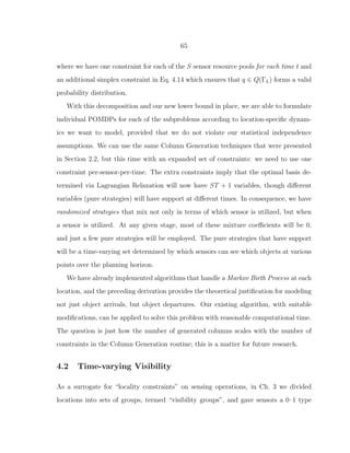
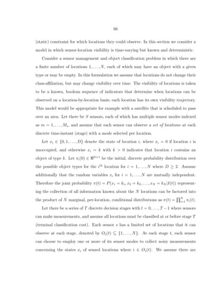
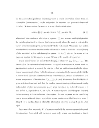
![68
is a resource cost rs(us(t)) to use this mode, representing power or some other type of
resource required to operate the sensor:
i∈Os(t)
rs(ui,s(t)) ≤ Rs ∀ s ∈ [1 . . . S]; ∀ t ∈ [0 . . . T − 1] (4.16)
This is a hard constraint for each sample-path: each and every possible realization
of observations and actions. There are no sensor resource dynamics per se because
resource availability at a later stage does not depend on resource expenditures at earlier
stages. There is however a time-varying demand for sensing resources according to when
the visibility constraints dictate are the best and worst times for observing locations.
These constraints model the limited information-processing bandwidth of sensors. The
S sensors are treated as a set of finite-capacity resource pools wherein making sensor
measurements consumes resources, however resources are renewed with every new time-
step; (aside from battery-powered devices), sensing-capacity is a renewable resource.
Concerning the set Os(t) of visible locations at stage t, consider the following dy-
namics: location i has a deterministic visibility profile, wi,s(t), for each sensor s that
is known a priori: wi,s : N+
→ {0, 1} where the indicator ‘1’ indicates the location is
visible. In this case, we assume that a sensor can look at a series of locations in any
order so long as the ordering preserves visibility constraints, so Os(t) = {i | wi,s(t) =
1, i ∈ [1, . . . , N]} ∀ s, t. The sensor platforms themselves have no physical state repre-
sentation. In this context, the action space is the set of all feasible sensor modes and
feasible sensing locations (for all sensors) at a particular time.
Let I(t) denote the sequence of past sensing actions and measurement outcomes up
to and including stage t − 1:
I(t) = {(ui,s(τ), ys,m(τ)) | i ∈ Os(τ); s = 1, . . . , S; τ = 0, . . . , t − 1}](https://image.slidesharecdn.com/9f5467db-22a0-4b25-9f85-d66c2d62a6f8-160910233158/85/dissertation-90-320.jpg)
![69
Define I(0) as the prior probability π(0) = p(x) = N
i=1 p(xi). Under the assumption
of conditional independence of measurements and independence of individual states at
each location, the joint probability π(t) = P(x1 = k1, x2 = k2, . . . , xN = kN |I(t))
can be factored as the product of belief-states (marginal conditional probabilities) for
each location. Denote the belief-state at location i as πi(t) = p(xi|I(t)). When a
sensor measurement is taken, the belief-state is updated according to Bayes’ Rule. A
measurement of location i with the sensor-mode combination ui,s(t) = (i, m) at stage t
that generates observable ys,m(t) updates the belief-vector as:
πi(t + 1) =
diag{P(ys,m(t)|xi = j, i, s, m)}πi(t)
1T
diag{P(ys,m(t)|xi = j, i, s, m)}πi(t)
(4.17)
where 1 is the D + 1 dimensional vector of all ones. Eq. 4.17 captures the relevant
information dynamics that SM controls through the choice of measurement actions.
The objective for this formulation is to classify, with minimum cost as measured by
FAs and MDs, the state of each location at the end of T stages:
J = min
γ∈Γ
E
γ
N
i=1
c(xi, vi) (4.18)
subject to Eq. 4.16.
After replacing the hard resource constraint in Eq. 4.16 with an expected-resource-
use constraint for each of the S sensors, we have the constraints:
i∈Os(t)
E[rs(ui,s(t))] ≤ Rs ∀ s ∈ [1 . . . S]; ∀ t ∈ [0 . . . T − 1] (4.19)
We can dualize the resource constraints and create an augmented objective-function
(Lagrangian) of the form:
Jλ = min
γ∈Γ
E
γ
N
i=1
c(xi, vi) −
S
s=1
T−1
t=0
λs(t)
Rs −
i∈Os(t)
rs(ui,s(t))
(4.20)](https://image.slidesharecdn.com/9f5467db-22a0-4b25-9f85-d66c2d62a6f8-160910233158/85/dissertation-91-320.jpg)

![72
Chapter 5
Adaptive Sensing with Continuous Action
and Measurement Spaces
In this chapter, we present an alternative approach for the inhomogeneous adaptive
search problems studied in [Bashan et al., 2007,Bashan et al., 2008] based on the con-
straint relaxation approach developed in [Casta˜n´on, 1997, Casta˜n´on, 2005b, Hitchings
and Casta˜n´on, 2010]. Our approach decomposes the global two-stage SM problem into
per location two-stage SM problems, coupled through a master problem for partition-
ing sensing resources across subproblems, which is solved using Lagrangian Relaxation.
The resulting algorithm obtains solutions of comparable quality to the grid search ap-
proaches proposed in [Bashan et al., 2007,Bashan et al., 2008] with roughly two orders
of magnitude less computation.
Whereas in Ch. 3 the computation went towards considering a relatively narrow
set of actions with a handful of possible observations over a long (deep) horizon, this
chapter considers a continuum of actions and observations with a shallower horizon.
In this chapter, the states of locations are binary-valued: X = {‘empty’, ‘occupied’}.
Therefore this chapter basically implements the ‘search’ mode of Ch. 3 for the shortest
horizon considered in that chapter but with a much higher resolution sensor model.
The remainder of this chapter proceeds as follows: Section 5.1 describes the two-stage
adaptive SM problem of [Bashan et al., 2007,Bashan et al., 2008]. Section 5.2 describes
our solution to obtain adaptive sensor allocation strategies. Section 5.3 discusses an](https://image.slidesharecdn.com/9f5467db-22a0-4b25-9f85-d66c2d62a6f8-160910233158/85/dissertation-94-320.jpg)
![73
alternative approach based on DP techniques. In Section 5.4, we provide simulation
results that compare our algorithms with the algorithms in [Bashan et al., 2008].
5.1 Problem Formulation
Consider an area that contains Q locations (or ‘cells’) to be measured with R total units
of resources (e.g. energy) over T = 2 stages indexed by t, starting with t = 0. Let the
cells be indexed by k ∈ [1, . . . , Q]. Define the indicator function Ik = 1 if the kth
cell
contains an object, and let Ik = 0 otherwise. The variables Ik are assumed to be random
and independent, with prior probability πk0 = Pr(Ik = 1).
The decision variables at stages t = 0, 1, are denoted by xkt, k = 1, . . . , Q, corre-
sponding to the sensor resource allocated to each cell k at stage t. As in [Bashan et al.,
2007,Bashan et al., 2008], allocating resources to a cell corresponds to allocating radar
energy to that cell, which improves the signal-to-noise ratio (SNR) of a measurement
there. A measurement generated for each cell k at stages 0, 1, is described by:
Ykt =
√
xktIk + vk(t) (5.1)
where vk(t) are Gaussian, zero-mean, unit variance random variables that are mutually
independent across k and t and independent of Ii for all i. Thus, xkt represents the energy
allocated to cell k at stage t and is also the signal-to-noise ratio for the measurement.
See Fig. 5·1 for a graphical depiction of this sensor model.
Let Yt = [Y1t, Y2t, . . . , YQt] denote the measurements collected across all locations at
stage t. For adaptive sensing, we allow the allocations xk1 to be a function of the ob-
servations Y0. Thus, an adaptive sensor allocation is a strategy γ = {(xk0, xk1(Y0)), k =
1, . . . , Q}. The resource (energy) constraint requires that feasible adaptive sensor allo-](https://image.slidesharecdn.com/9f5467db-22a0-4b25-9f85-d66c2d62a6f8-160910233158/85/dissertation-95-320.jpg)
![74
−6 −4 −2 0 2 4 6 8 10 12
0
0.05
0.1
0.15
0.2
0.25
0.3
0.35
0.4
Likelihood functions p(Y
k0
| I=1; x
k0
=[0.81 2.83 5.66 ]) and p(Y
k0
|I=0)
yk0
p(Y
k0
|I;x
k0
)
Figure 5·1: Depiction of measurement likelihoods for empty and non-empty
cells as a function of xk0.
√
xk0 gives the mean of the density p(Yk0|Ik = 1). If
the cell is empty the observation is always mean 0 (black curve).
cations satisfy:
Q
k=1
(xk0 + xk1(Y0)) ≤ R for all Y0 (5.2)
Note, the resulting optimization problem has a continuum of constraints for all sample
paths of the observations Y0.
We initially use the following cost function, from [Bashan et al., 2007,Bashan et al.,
2008], to develop an adaptive sensing strategy:
Jγ
= E
γ
Q
k=1
Ik
xk0 + xk1(Y0)
(5.3)
This cost function rewards allocating more sensing resources to cells that are occupied.
There are many other variations that can be considered, but this simple form is sufficient
to illustrate our approach.
The above problem can be solved in principle using SDP, but the cost is not easily
separable across stages. Nevertheless, one can still use nested expectation principles to](https://image.slidesharecdn.com/9f5467db-22a0-4b25-9f85-d66c2d62a6f8-160910233158/85/dissertation-96-320.jpg)
![75
Figure 5·2: Waterfall plot of joint probability p(Yk0|Ik; xk0) for πk0 = 0.50
for xk0 ∈ [0 . . . 20]. This figure shows the increased discrimination ability that
results from using higher-energy measurements (separation of the peaks).
approach this problem, as outlined in [Bashan et al., 2008]. Define the belief-state:
πk,t+1 = P(Ik = 1|Yt) = P(Ik = 1|Ykt), k = 1, . . . , Q (5.4)
and resource dynamics:
R1 = R −
Q
k=1
xk0
where the last equality in Eq. 5.4 follows from the independence assumptions made on
the cell indicator functions and the measurement noise. Fig. 5·2 is a 3D plot displaying
how increasing energy expenditures improves the discriminatory power of sensor mea-
surements (improves SNR), and Fig. 5·3 demonstrates how this increased discriminatory
power affects the resulting a posteriori probability for a cell, πk1.](https://image.slidesharecdn.com/9f5467db-22a0-4b25-9f85-d66c2d62a6f8-160910233158/85/dissertation-97-320.jpg)
![76
Figure 5·3: Graphic showing the posterior probability πk1 as a function of
the initial action xk0 and the initial measurement value Yk0. This surface plot
is for λ = 0.01 and πk0 = 0.20. (The boundary between the high (red) and low
(blue) portions of this surface is not straight but curves towards -y with +x.)
Let πt = [π1t, . . . , πQt], x0 = [x10, . . . , xQ0], x1 = [x11, . . . , xQ1]. Then:
min
γ
Jγ
= min
γ
E
γ
Q
k=1
Ik
xk0 + xk1(Y0)
= min
x0
E min
x1(Y0)
E
Q
k=1
Ik
xk0 + xk1(Y0)
Y0
= min
x0
E E min
x1
Q
k=1
Ik
xk0 + xk1(Y0)
Y0
= min
x0
E min
x1
Q
k=1
πk1
xk0 + xk1
(5.5)
For each value of x0 and measurements Y0, the inner minimization is a deterministic
resource allocation problem with a convex, separable objective and a single constraint
Q
k=1 xk1 = R − Q
k=1 xk0, which is straightforward to solve. The algorithm of [Bashan
et al., 2008] then solves the overall problem by enumerating possible values of x0, simu-](https://image.slidesharecdn.com/9f5467db-22a0-4b25-9f85-d66c2d62a6f8-160910233158/85/dissertation-98-320.jpg)
![77
lating values of Y0 for each x0 and subsequently solving the inner minimization problem
for each x0, Y0 combination to find the best set of adaptive sensor allocations.
5.2 Relaxed Solution
In order to avoid enumeration of all feasible resource allocations at stage 0, we adopt a
constraint relaxation approach that expands the space of feasible sensor allocations, as
in Section 2.2 and [Casta˜n´on, 1997,Casta˜n´on, 2005b]. Specifically, we approximate the
constraints implied by Eq. 5.2 with a single resource constraint that constrains the total
expected energy use:
E
Q
k=1
(xk0 + xk1(Y0)) ≤ R, xkt ≥ 0 (5.6)
This expands the space of admissible sensor allocations, so the solution of the SM prob-
lem with these constraints yields a lower bound to the original problem. We introduce
a Lagrange multiplier λ ≥ 0 to integrate this constraint into an augmented objective
function:
Jγ
(λ) =
Q
k=1
E
Ik
xk0 + xk1(Y0)
+ λ E
Q
k=1
(xk0 + xk1(Y0)) − R (5.7)
Given λ, Eq. 5.7 is additive over the cells, so for the remainder of this chapter we
concentrate on the cost of optimally classifying just one cell. This separability establishes
the following result:
Theorem 5.2.1. An optimal solution of Eq. 5.7 subject to constraints Eq. 5.6 is achieved
by an adaptive sensing strategy where xk1(Y0) ≡ xk1(Yk1) ≡ xk1(πk1).
The proof of this follows along the lines of the results in [Casta˜n´on, 2005b,Castanon
and Wohletz, 2009]. This result restricts the adaptive sensing allocations for each cell k
to depend only on the information collected on that cell, summarized by πk1, and leads](https://image.slidesharecdn.com/9f5467db-22a0-4b25-9f85-d66c2d62a6f8-160910233158/85/dissertation-99-320.jpg)

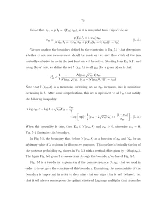
![80
Figure 5·4: Cost function boundary (see Eq. 5.14) with λ = 0.011 and
πk0 = 0.18. In the lighter region two measurements are made, in the darker
region just one. (Note positive y is downwards.)
Figure 5·5: The optimal boundary for taking one action or two as a function
of (xk0, Yk0) (for the [Bashan et al., 2008] cost function) for λ = 0.01 and
πk0 = 0.20. The curves in Fig. 5·6 represent cross-sections through this surface
for the 3 x-values referred to in that figure.](https://image.slidesharecdn.com/9f5467db-22a0-4b25-9f85-d66c2d62a6f8-160910233158/85/dissertation-102-320.jpg)
![81
−6 −4 −2 0 2 4 6 8 10 12
−15
−10
−5
0
5
10
Measurement Boundry for Having/Not−Having Follow−up
Action for xk0
=[0.81 2.83 5.66 ] λ=0.0100 p=0.20
yk0
γ(xk0
,λ)
Figure 5·6: This figure gives another depiction of the optimal boundary
between taking one measurement action or two for the [Bashan et al., 2008]
cost function. For all Y (xk0, λ) ≥ 0 two measurements are made (and the
highest curve is for the smallest xk0, see Fig. 5·5 for the 3D surface from which
these cross-sections were taken).
the individual subproblems.
We now develop an expression for the outer expectation in Eq. 5.8, which defines the
problem of optimizing xk0, as follows: let p(yk0; xk0) = p(Yk0|Ik = 1; xk0)πk0 +p(Yk0|Ik =
0; xk0)(1 − πk0). Then using Eq. 5.13 yields:
E[Jλ∗
k,1(xk0, πk1)] =
y∈Y (xk0,λ)
2 λπk1 p(yk0; xk0)dyk0
+
y /∈Y (xk0,λ)
πk1
xk0
+ λxk0 p(yk0; xk0)dyk0
=
y∈Y (xk0,λ)
2 λπk0 N(yk0;
√
xk0, 1) p(yk0; xk0)dyk0
+
y /∈Y (xk0,λ)
πk0
xk0
N(yk0;
√
xk0, 1) + λxk0 p(yk0; xk0) dyk0
To minimize E[Jλ∗
k,1(xk0, πk1)] with respect to xk0, we have to evaluate the integrals
above. Note, the regions of integration also depend on xk0. Although it is possible](https://image.slidesharecdn.com/9f5467db-22a0-4b25-9f85-d66c2d62a6f8-160910233158/85/dissertation-103-320.jpg)
![82
Figure 5·7: Two-factor exploration to determine how the optimal boundary
between taking one measurement or two measurements varies for a cell with
the parameters (p, λ) where p = πk0 (for the [Bashan et al., 2008] problem cost
function). Two measurements are taken in the darker region, one measurement
for the lighter region.](https://image.slidesharecdn.com/9f5467db-22a0-4b25-9f85-d66c2d62a6f8-160910233158/85/dissertation-104-320.jpg)
![83
to take derivatives and try to solve for possible minima, it is simpler to evaluate the
integrals by numerical quadrature and obtain the optimal value xk0 by numerical search
in one dimension.
The above procedure computes the optimal strategy for the relaxed problem of
Eq. 5.7 for fixed λ. To obtain a solution to the original problem with the relaxed
constraints of Eq. 5.6, we do an optimization over λ: a one-dimensional concave max-
imization problem where the direction of ascent is readily identified. A subgradient
direction is given by:
∂Jγ
(λ) = E
Q
k=1
(xk0 + xk1(Y0)) − R
=
Q
k=1
y∈Y (xk0,λ)
πk1
λ
p(yk0; xk0)dyk0
+
Q
k=1
y /∈Y (xk0,λ)
xk0 p(yk0; xk0)dyk0 − R
Note, the relevant expectations have already been evaluated by quadrature in the search
for the optimal xk0 for each λ, which makes searching for the optimal λ straightforward.
The algorithm above obtains optimal adaptive sensor allocations for optimizing
Eq. 5.3 subject to the relaxed constraints in Eq. 5.6. To obtain sensor allocations
that satisfy the original constraints of Eq. 5.2, we use the sensor allocations {xk0, k =
1, . . . , Q} determined by our procedure above, collect the vector of observations Y0 across
all cells, and then replan for the optimal allocation of the remaining resources, enforcing
the constraint Eq. 5.2 for the specific observations Y0. This stage 1 optimization problem
is a straightforward deterministic separable convex minimization problem with a single
additive constraint, and can be solved analytically in finite time by indexing the cells,
as described in [Bashan et al., 2008].](https://image.slidesharecdn.com/9f5467db-22a0-4b25-9f85-d66c2d62a6f8-160910233158/85/dissertation-105-320.jpg)
![84
5.3 Bayesian Objective Formulation
One of the factors that makes the adaptive SM problem in [Bashan et al., 2008] complex
is that the objective function Eq. 5.3 does not depend on the observed measurements at
stage 1, Y1. As argued in [Bashan et al., 2008], this objective is related to lower bounds
in performance such as Cramer Rao bounds on the estimation of Ik or Chernoff bounds
on correct classification, particularly for open-loop allocations. The resulting cost is not
separable across stages, and is a hybrid of bounds and actual expected performance.
A direct approach would have been to define a cost at stage 2 that depends on the
measurements of both stages 0 and 1, along with a decision stage that generates an
estimate or a classification for each cell, as in [Casta˜n´on, 2005b], and to use DP tech-
niques for partially observed Markov decision processes (POMDPs), suitably extended
to incorporate continuous-valued action and measurement spaces.
We assume that for each cell k at stage 2 there will be a classification decision uk2 ∈
{0, 1}, which depends on the observed measurements Y0, Y1. For any cell k where we have
collected Yk0, Yk1, denote the conditional probability πk2 = P(Ik = 1|Yk0, Yk1; xk0, xk1).
Let MD denote a constant representing the relative cost of a missed detection at the
end of 2 stages where the false alarm cost (FA) is held constant at 1. The Bayes’ cost
we seek to optimize is:
JBayes
= E
Q
k=1
(MD Ik(1 − uk2) + (1 − Ik)uk2)
The surfaces of Fig. 5·8 show how the MD and FA costs vary with the values of xk1
and Yk1 after making the first measurement. These figures are cost-samples for the cost
that results after each outcome (xk1,Yk1) at the last stage. The FA classification cost
is independent of the amount of energy used in the second measurement, but the MD
classification cost is not.](https://image.slidesharecdn.com/9f5467db-22a0-4b25-9f85-d66c2d62a6f8-160910233158/85/dissertation-106-320.jpg)
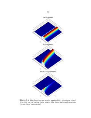
![86
Incorporating the relaxed constraints of Eq. 5.6, we get an augmented cost that can
be decomposed over cells, along the lines of the formulation in the previous section, to
obtain the cell-wise optimization objective:
JBayes
k (λ) = E[(MD Ik(1 − uk2) + (1 − Ik)uk2) + λ(xk0 + xk1)]
where xk1 depends on Yk0, and uk2 depends on Yk0, Yk1. Using DP, the sufficient statistic
for this problem is the information state πkt for each stage t. The cost-to-go at stage 2
is:
J∗
k,2(πk2) = min MD πk2, (1 − πk2)
The DP recursion is now:
Jλ∗
k,1(πk1) = min
xk1
E min MD
p(Yk1|1; xk1)πk1
p(Yk1; xk1)
, (1 −
p(Yk1|1; xk1)πk1
p(Yk1; xk1)
) + λxk1 (5.15)
Using this DP recursion yields the optimization problem for xk0:
min
xk0
E Jλ∗
k,1(πk1) + λxk0
Fig. 5·9 shows a set of plots for the Bayes’ cost function when t = 1 for the proba-
bilities πk1 = 0.0991 and πk1 = 0.3493 for λ = 0.0001. The first row in the figure
shows cost-samples for the unaugmented cost function, the middle row for Eq. 5.15 and
the final row shows the corresponding joint-probabilities for each prior. These figures
demonstrate that the higher the value of πk1, the larger the amount of cost associated
with a measurement Yk1 that is near 0 (the measurement is ambiguous and so the chance
of making a mistake and paying a classification cost is relatively large). Fig. 5·10 de-
scribes the boundary between determining a cell to be empty / occupied for the Bayes’
cost function with γ(xk1) defined as the observation value Yk1 that makes the FA and
MD costs equal.](https://image.slidesharecdn.com/9f5467db-22a0-4b25-9f85-d66c2d62a6f8-160910233158/85/dissertation-108-320.jpg)
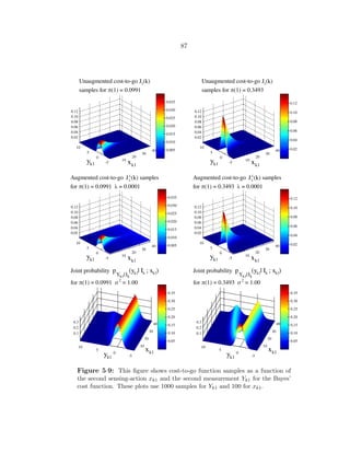
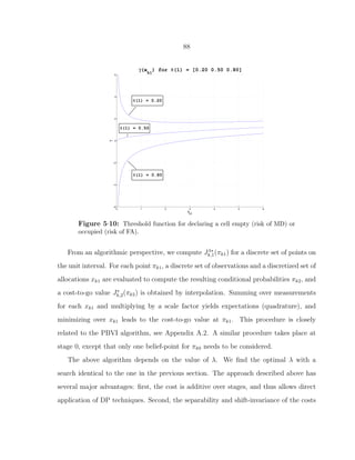
![89
allows for computation of a single cost-to-go function Jλ∗
k,1(πk1) for all cells k, which is a
significant savings in computation.
5.4 Experiments
We now consider some simulation results. Simulations were done using MATLAB on
a 2.2 Ghz, single-core, Intel P4, Linux machine. We ran two separate simulation con-
figurations. The first was an independent experiment and the second was meant to be
compared against the algorithm of [Bashan et al., 2007,Bashan et al., 2008].
In the first configuration, we used 1000 points to discretize the observation space
for quadrature, 100 discrete points to search for optimal sensor allocations xk0 with a
line search and 500 units of energy, which gives an SNR (= 10 log10 (R
Q
)) of 6.99 units.
The values reported in the experiments are averages over 100 simulation runs using
Q = 100 cells. A set of prior probabilities was created for the 100 simulations using
100 independent samples from a gamma distribution with shape 2 and scale 3. The
values were scaled and thresholded to fall in the range [0.05 . . . 0.80]. The net result was
a vector of prior probabilities with most of its values around 0.10 − 0.20 and with a few
higher probability elements.
We first focus on comparing the adaptive sensor allocation algorithm using the re-
laxation approach of Section 5.2. Fig. 5·11 displays the initial resource allocation as a
function of the value of the prior probability of each cell πk0. The amount of resource
initially allocated to measuring a cell is a monotonically increasing function of the chance
that an object is there, as the cost function rewards spending resources on cells that
contain objects. Fig. 5·12 shows a similar behavior for the total expected resource alloca-
tions per cell (with the expected value of the follow-up resource allocations (xk1) making
up the difference between Fig. 5·11 and Fig. 5·12). The striations seen in Fig. 5·11 are
artifacts of the resource allocation quantizations at stage 0, which had a granularity of](https://image.slidesharecdn.com/9f5467db-22a0-4b25-9f85-d66c2d62a6f8-160910233158/85/dissertation-111-320.jpg)
![90
around 0.2 units of energy. There are more points on these graphs for small values of πk0
because a prior was used with a relatively low probability of object occurrence. Fig. 5·13
is very similar to Fig. 5·12 because the classification cost is completely determined by
the total amount of resource spent and the prior probability of an object being present.
In terms of computation time, determining the optimal adaptive sensor allocation (for
0 0.1 0.2 0.3 0.4 0.5 0.6 0.7 0.8
2
2.5
3
3.5
4
4.5
5
5.5
6
π(0)
energy
First Stage Energy Allocation vs Prior Probability
Figure 5·11: The 0th stage resource allocation as a function of prior prob-
ability. The striations are an artifact of the discretization of resources when
looking for optimal xk0.
the case of non-uniform priors) required around two minutes for our MATLAB imple-
mentation. Subsequent evaluation of the performance using Monte Carlo runs required
around 10 seconds per simulation. To summarize the performance statistics, the aver-
age simulation cost over 100 simulations was 2.85 units, and the sample variance of the
simulation cost was 0.40 units.
In order to compare our results with the results of [Bashan et al., 2008] for the second
simulation configuration, we obtained a MATLAB version of their algorithm with a](https://image.slidesharecdn.com/9f5467db-22a0-4b25-9f85-d66c2d62a6f8-160910233158/85/dissertation-112-320.jpg)
![91
0 0.1 0.2 0.3 0.4 0.5 0.6 0.7 0.8
2
3
4
5
6
7
8
9
10
11
π(0)
energy
Total Energy Allocation vs Prior Probability
Figure 5·12: Total resource allocation to a cell as a function of prior proba-
bility. The point-wise sums of the 0th stage and 1st stage resource expenditures
are displayed here.
specific problem implementation that contained a grid of Q = 1024 cells and used an
action space discretized to 100 energy levels. Their algorithm evaluated expectations
using 500 random samples for Y0. We used 1000 energy levels and an observation space
discretized to 100 observations. The algorithms in [Bashan et al., 2008] assume a uniform
prior probability πk0 = 0.01, which reduces the need for a Q-dimensional enumeration
to a one dimensional enumeration because of symmetry, so xk0 is constant across all
cells k. To get an overall SNR of 10, the resource (energy) level R was set to 10240
so that, on average, there are 10 units of resources per cell. We used 100 Monte Carlo
simulations to evaluate the performance of the adaptive sensor allocations.
With this second configuration involving an order of magnitude more cells, our MAT-
LAB algorithm created an adaptive sensor allocation plan in 9.5 seconds by exploiting
the symmetry across cells. Evaluation of performance with the 100 Monte Carlo simu-](https://image.slidesharecdn.com/9f5467db-22a0-4b25-9f85-d66c2d62a6f8-160910233158/85/dissertation-113-320.jpg)
![92
0 0.1 0.2 0.3 0.4 0.5 0.6 0.7 0.8
0.02
0.04
0.06
0.08
0.1
0.12
0.14
π(0)
cost
Cost vs Prior Probability
Figure 5·13: Cost associated with a cell as a function of prior probability. For
the optimal resource allocations, there is a one-to-one correspondence between
the cost of a cell and the resource utilized to sense a cell.
lations required an additional 17.7 seconds to do the 100 simulations. We ran the same
experiments using the MATLAB code implementing the approach described in [Bashan
et al., 2008], which required 100.3 sec to compute adaptive sensor allocations, and 2.7 sec
of simulation time to evaluate performance (because their algorithm does not require in-
line replanning to ensure feasibility). The results are summarized in Table I. The results
show that our algorithm achieves performance close to that of the optimal algorithm
described in [Bashan et al., 2008] with significantly lower computational requirements.
The above comparison does not highlight the fact that our algorithm is scaleable
for problems with non-uniform prior information. In essence, for our algorithm non-
uniform priors would increase computation time by a factor of Q, the number of distinct
cells that require evaluation using our relaxation approach. In contrast, computation
times for the algorithm of [Bashan et al., 2008] would require enumeration of 1024Q](https://image.slidesharecdn.com/9f5467db-22a0-4b25-9f85-d66c2d62a6f8-160910233158/85/dissertation-114-320.jpg)
![93
Average Standard Solution Simulation
Cost Deviation Time Time
Relaxation 0.2762 0.14 9.5 17.7
Exact 0.2666 0.15 100.3 2.7
Table 5.1: Performance comparison averaged over 100 Monte Carlo simu-
lations. Relaxation is the algorithm proposed in this chapter, while Exact
is the algorithm of [Bashan et al., 2008]
0 0.1 0.2 0.3 0.4 0.5 0.59 0.69 0.79 0.89 0.99
0
0.01
0.03
0.05
0.07
0.09
0.1
0.12
0.14
0.16
0.17
π1
(k)
J
λ
1
(k)
Figure 5·14: Cost-to-go from πk1
locations versus 1024 locations, an exponential increase in time, making consideration
of nonuniform priors an infeasible problem.
As a final set of experiments, we implemented the algorithm of Section 5.3 using the
first simulation configuration with 100 cells and MD = 1. We used a grid of 1000 belief-
points to represent the cost-to-go function, with cubic spline interpolation for values in
between points. The optimal cost-to-go at stage 1 in the Bayes’ cost function is shown in
Fig. 5·14 and the corresponding optimal energy allocations are in Fig. 5·15. The results
show the expected cutoff where no action is taken once enough certainty exists in πk1.](https://image.slidesharecdn.com/9f5467db-22a0-4b25-9f85-d66c2d62a6f8-160910233158/85/dissertation-115-320.jpg)
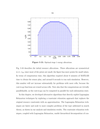
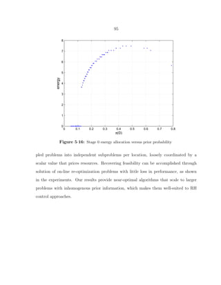

![98
around them will have evolved into a new state that is not necessarily related to the
one for which a decision is to be made. If humans are forced to act too quickly, they
may not be able to outperform machine systems, and therefore lose their utility in a
semi-autonomous system. In order to close the loop and allow robots to collaborate
with humans, algorithms used for machine-reasoning need to incorporate an awareness
of the time-scale that humans require for choosing courses of action.
Tasking humans with decision-making at a time-scale that is at or near the limits
of their capability only detracts from human situational awareness and leaves humans
prone to making poor decisions. Time-scales appropriate for human interaction need to
be established as a function of current and projected near-term environmental complex-
ity and need to include the fixed-cost of asking a human operator to switch contexts as
well as the time-cost of analyzing a situation to reach a decision. The relative benefit
of human supervision must be weighed against how well a machine can perform inde-
pendently and an awareness of what else the human could have been doing with that
time. This problem is similar to a job-scheduling problem with stochastic setup and job-
completion times where the “servers” are human operators. (See [Leung, 2004,Sellers,
1996] for an overview of job-shop scheduling problems).
6.1.3 Human and Machine Strengths and Weaknesses
Whereas humans are capable of significant parallel processing (e.g. w.r.t. being aware
of and responding to numerous novel stimuli at the same time), they do so on a very
slow time-scale relative to autonomous agents. However, automata are typically built
to perform just a few select tasks very well and at high-speed; developing algorithms
that have generalization capability remains a serious challenge. Humans can currently
identify patterns and trends in complex environments that far exceed the ability of any
automaton to process. On the other hand, humans are fallible, can become bored or](https://image.slidesharecdn.com/9f5467db-22a0-4b25-9f85-d66c2d62a6f8-160910233158/85/dissertation-120-320.jpg)
![99
confused and can act with predilection or supposition or short-sightedness. The larger
the task that a human is given, the more contextual information there is to be aware of,
the longer it takes human operators to switch between tasks [Cummings and Mitchell,
2008]. Therefore this is a design parameter, and tasks need to be divided up into
appropriately sized pieces to maximize human operator effectiveness.
One of the largest problems with incorporating input from human operators that
oversee multiple robotic vehicles is that it is easy to confuse contexts in switching be-
tween tasks and in so doing, to lose situational awareness [Cummings et al., 2005]. If
human agents become confused, they are rendered idle until re-situated. The higher
the complexity of the mission-space and the more dynamic the state-space, the more
likely such loss of awareness is to happen. However, this issue can be quantified and
anticipated, which allows for potential problems to be in large part averted. One
means of staving off these problems is by providing human operators with key fea-
tures/indicators when switching tasks such that information is presented to humans on
a need-to-know/prioritized basis (with a certain amount of redundancy).
There is a duality relationship between man and machine that can be exploited.
Humans can help automata perform better by adding domain-specific knowledge that
is not yet modeled (or feasible to model) in machine planning algorithms. Human par-
ticipants in the decision-making loop can employ higher level reasoning processes (e.g.
handling of contingency scenarios when a vehicle falls out of commission) to add robust-
ness and human experience to the search and exploitation process. A semi-autonomous
hybrid controller can take the input from both human and non-human controllers and
fuse it together in such a way as to leverage the strongest characteristics of each of the
component controllers.](https://image.slidesharecdn.com/9f5467db-22a0-4b25-9f85-d66c2d62a6f8-160910233158/85/dissertation-121-320.jpg)
![100
6.1.4 Time-Varying Machine Autonomy
It is of practical interest to try and develop semi-autonomous object search and exploita-
tion algorithms that can operate at dynamic levels of autonomy according to mission
complexity [Bruemmer and Walton, 2003, Baker and Yanco, 2004, Schermerhorn and
Scheutz, 2009,Goodrich et al., 2001]. The goal is to keep human workload at an accept-
able level at the busiest of times while not forgoing the performance enhancements that
humans can provide a semi-autonomous control system at less busy times. In routine
conditions, a semi-autonomous system may be able to proceed on “autopilot” whereas in
dangerous situations, or ones in which there is a lot of uncertainty/rapidly changing en-
vironmental conditions, it may be advantageous for humans to step in and assume more
authority over UAV activities. It is obviously very important that any robot operating
in the field be able to quantify its degree of uncertainty about the external environment
and “understand” when its model for the world isn’t matching reality.
6.1.5 Machine Awareness of Human Inputs
The amount of input that a human operator can give to numerous vehicles communicat-
ing on a one-on-one basis is limited, so the duration and objective of these interactions
needs to be delimited by a protocol that is adaptive to circumstances [Cummings et al.,
2005]. Allowing humans to participate in search and exploitation missions requires de-
veloping sophisticated Graphical User Interfaces (GUI’s) that present a dynamic flow of
information that is filtered/emphasized in real-time according to the content of the data
being displayed. In order to best leverage humans’ cognitive abilities for prediction, in-
tuition and pattern-recognition, it is necessary to design software that takes account of
the relative importance of the information being displayed and how long a human will re-
quire in order to grasp and make use of that information [Kaupp and Makarenko, 2008].
If human operators do not have sufficient time to consider and react to information that](https://image.slidesharecdn.com/9f5467db-22a0-4b25-9f85-d66c2d62a6f8-160910233158/85/dissertation-122-320.jpg)
![101
is displayed to them, that information becomes noise that impairs the completion of
other (feasible) tasks, and it should not be displayed [Cummings et al., 2005]. There
is also a potential schism that must be handled concerning the activities a human may
wish to focus on versus what a predictive decision-making algorithm considers to be the
most important issue for human operators to work on.
6.2 Control Structures for HRI
There are several degrees of freedom to be explored when it comes to the control struc-
tures that are used to regulate, route, sequence and validate decisions made by machines.
The number of robotic agents that a single human can oversee while acting as a supervi-
sor is a central issue to explore [Cummings and Mitchell, 2008,Steinfeld et al., 2006]. In
addition to using humans in a supervisory capacity, human operators can act as peers
within a semi-autonomous team. Humans can also assume control of robots in time-
varying fashion as a situation warrants. For instance 3 humans could oversee 9 robots
(in 3 subgroups) and a 4th
human could be tasked to assist one of the 3 subgroups
in time-varying fashion as needed. Up to a certain level of dynamism in the environ-
ment, this would allow all 3 subgroups to reap most of the benefits of having 2 human
decision-makers involved at all times [Nehme and Cummings, 2007].
In addition to exploring the best choice for optimal team size and composition, the
tasks that human/non-human operators perform best can vary over time. Tasks can
be partitioned according to several different static and dynamic strategies [Gerkey and
Matari´c, 2004]. As a first pass, a catalog of activities can be created, and then hu-
mans can be given a fixed subset of the activities that they perform well and robots the
complementary subset. Tasks can be partitioned between humans and machines based
upon geographical constraints, which makes sense if humans are navigating vehicles and
doing their own information-gathering. Tasks can preferentially be given to a human](https://image.slidesharecdn.com/9f5467db-22a0-4b25-9f85-d66c2d62a6f8-160910233158/85/dissertation-123-320.jpg)
![102
(machine) decision-maker and robots (humans) can be used as a fall-back option. Dif-
ferent humans have heterogeneous capabilities and robots may as well. Task-allocations
should take such heterogeneity into account [Nehme and Cummings, 2007]. Tasks can
be partitioned based on a time-window threshold at which point humans will not have
enough time to accomplish the task, so therefore a robot must take responsibility. Tasks
can be allocated based on situational awareness metrics that machines use to gauge hu-
man preparedness [Cummings et al., 2005]. Decisions must be made in a collaborative
fashion, however, such that human and non-human decisions complement each other
versus impede each other [Dudenhoeffer, 2001]. A mixed initiative control mechanism is
necessary in order to incorporate both robot and human decisions into a single, unified
plan of action. Human operators may be able to quickly generate a few candidate plans
of action without being able to determine which one is best. If people can help “narrow
the playing field” for autonomous agents, the agents can concentrate their processing
power on looking more deeply into such a refined/limited set of strategies.
In as much as possible, it is desirable to use a policy-driven decision-making scheme
wherein a human makes a standing decision that remains in effect unless preempted by
another human or a more important decision. “Management by exception” is required
in order to support a system with one human controlling large numbers of robots [Cum-
mings and Morales, 2005]. Threshold policies and quotas concerning resource usage and
rate of usage are types of policies that both humans and non-humans can use to good
effect. We explore how these decision-making techniques can be exploited to relieve
the decision-making burden on human-operators but at the same time keep them as
informed as possible about the evolving state of a mission.](https://image.slidesharecdn.com/9f5467db-22a0-4b25-9f85-d66c2d62a6f8-160910233158/85/dissertation-124-320.jpg)
![103
6.2.1 Verification of Machine Decisions
Autonomous agents have yet to become fully accepted as team-members alongside hu-
mans in a collaborative environment. This issue has been observed in search and rescue
settings as well as military ones. It takes time for people to gain confidence in new
technology [Cummings et al., 2005]. In order to facilitate the acceptance process of
autonomous agents, it is necessary to build machine-reasoning algorithms that not only
arrive at verifiably good decisions, but ones that are transparent to a human opera-
tor. The issue of not over-trusting or under-trusting automata is a key factor in system
performance [Freedy et al., 2007].
In short, we seek to consider the performance benefits of including one or more hu-
mans in the SM decision-making loop to guide the actions of semi-autonomous vehicles.
We seek to identify tasks that robots do not perform well, that are computationally
intractable for automata, or where machines would benefit from an external informa-
tion source. Incorporating human input increases robustness to model error, allows the
system to be capable of handling anomalies that are outside the scope of its design, and
adds a level of redundancy that ensures the robots remain grounded and on track at
all times. Conversely, having computerized feedback from robots can help the humans
remain situated at all times as well.
6.3 Strategy Game Design
Having discussed some of the issues concerned with human supervisory control of teams
of robots, this section describes how human operators may enhance the performance of
our search and exploitation system. In preceding chapters we have developed algorithms
that allow robots operating in dynamic environments of limited size to conduct near-
optimal search and exploitation activities. In order to create an algorithm for SM over
extended distances, we use a game that explores using a human supervisor to coordinate](https://image.slidesharecdn.com/9f5467db-22a0-4b25-9f85-d66c2d62a6f8-160910233158/85/dissertation-125-320.jpg)
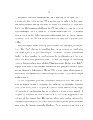
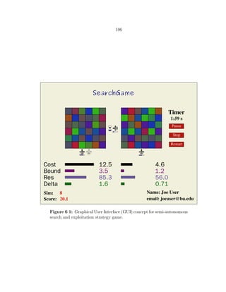


![111
Chapter 7
Conclusion
Viewed from a high-level, this dissertation seeks to address outstanding problems in the
domain of optimal search theory with follow-up actions, the trade-off between search
versus exploitation and human-computer relations/human-factors. Within this context,
we have presented algorithms that allow large, combinatorially complex problems to
be broken up into subproblems of a tractable size that can be solved in real-time. We
perform these hierarchical decompositions using Lagrangian Relaxation and Column
Generation to coordinate the solutions of independently-solved subproblems without
losing the fidelity represented in subproblem solutions.
7.1 Summary of Contributions
In one of the most important contributions of this dissertation, Ch. 3 describes novel
techniques for RH control algorithms based on mixed strategies and a lower bound for
sensing performance that was developed in [Casta˜n´on, 2005a,Casta˜n´on, 2005b]. These
strategies consider near-optimal (non-myopic, adaptive) allocation schemes for a set of
noisy, multi-modal, heterogeneous sensors to detect and classify objects in an unknown
environment in the face of resource constraints using a centralized control algorithm.
We consider mixed strategies for sensing that employ a handful of possible sensor modes
and a discrete set of measurement symbols with deep (far-seeing) decision-trees.
A C++/C-language simulator was constructed to implement our RH control algo-
rithms, and simulations using fractional factorial design of experiments were performed.](https://image.slidesharecdn.com/9f5467db-22a0-4b25-9f85-d66c2d62a6f8-160910233158/85/dissertation-133-320.jpg)
![113
more general version of the problem that was posed by [Bashan et al., 2007] in roughly
two orders of magnitude less computing time. First and foremost we avoid performing
N dimensional grid-searches while looking for the optimal per-location sensing energy
allocations. Lagrangian Relaxation and Duality theory are harnessed for this purpose.
We make the argument that these decomposition methods as proposed by [Yost and
Washburn, 2000, Casta˜n´on, 2005a, Casta˜n´on, 2005b] can be applied to a wide-range of
problems involving search, classification, (sensor) scheduling and assignment problems
of which Ch. 3 and Ch. 5 provide prototypical examples.
The final contribution of this dissertation consists of the design of a game that ex-
plores issues surrounding the best means of allowing humans (operators) to input feed-
back into a semi-autonomous system that performs search+exploitation functions with
the ultimate goal of developing a near-optimal, mixed initiative, human+robot search
team that leverages the strengths of machine algorithms (model predictive control with
scripted intelligence) and human intelligence (real-time feedback and adaptation). We
propose the design of this game as a means of empirically measuring the most informa-
tive type of GUI interface for human operators that maximizes situational awareness
and minimizes operator workload. Such a design allows more robots to be controlled
per human operator.
7.2 Directions for Future Research
There are numerous directions for future work in the domain of SM. First of all, the
algorithms we have proposed for RH control using time-varying Lagrange multipliers
could be implemented. Column generation is known to have slow convergence properties
for large problem instances, so the question of how these algorithms scale in the context
of strategies that randomize sensor utilization over sensors and time (i.e. many more
multipliers) is of interest.](https://image.slidesharecdn.com/9f5467db-22a0-4b25-9f85-d66c2d62a6f8-160910233158/85/dissertation-135-320.jpg)
![114
The implementation of a game such as the one we have designed to explore the
best framework for human supervisory control of robots is another important direction
of inquiry. The ultimate goal being the creation of a mixed-initiative system wherein
humans are maximally aware of what the automata are doing, robots are well-situated
w.r.t. the situational awareness of their human operators, multiple human operators
are able to communicate essential information between themselves, and all parties are
continually tasked with activities that they are well-suited to perform. Robots that
support adaptive autonomy levels are a topic of much interest recently. Ideally automata
will be self-sufficient when humans are already over-loaded with other tasks but still
designed to be able to incorporate more fine-grained human input when it is available.
Robots that are managed by exception and that do not need explicit instructions for
each and every task they perform are a long term goal in the Human-Robot Interaction
domain and in the domain of human-assisted search and exploitation.
A system for search and exploitation that jointly performs near-optimal SM and
path-planning would be a direct though non-trivial extension of this research. We are
interested in a problem paradigm that does not attribute value to moving a sensor to a lo-
cation, but moving a sensor to be within sight of a location. After developing a tractable
algorithm for SM with path-planning, a paradigm with risk of platform loss/malfunction
can be considered. A near-optimal and adaptive algorithm for decentralized SM would
be a significant contribution as well. Tractable algorithms for near-optimal SM with
moving targets are interesting and difficult problems to work on.
Higher resolution sensor models (more subproblem resolution [Jenkins, 2010]) and
support for correlated sensor observations could be investigated. The models we have
discussed in this work are appropriate for sensors that make observations with a narrow
FOV (e.g. an electro-optical camera with a telephoto lens). Alternatively, research could
be conducted for problems where sensors make observations over extended areas at the](https://image.slidesharecdn.com/9f5467db-22a0-4b25-9f85-d66c2d62a6f8-160910233158/85/dissertation-136-320.jpg)

![116
Appendix A
Background Theory
In this appendix we briefly overview some of the theory and concepts used in this
dissertation. We first summarize the definition of a POMDP model and describe how
the Witness Algorithm or PBVI can be used to solve POMDPs. Next, we discuss
Dantzig-Wolfe Decompositions and Column Generation as a special case.
A.1 Partially Observable Markov Decision Processes
A Markov Decision Process (MDP) is a dynamic decision problem where the underlying
state evolution is modeled by a Markov process, controlled by the decisions, and the state
is perfectly observed and used as the basis for making adaptive decisions. There are a
wide variety of uses for MDPs, some of which are discussed in [Bertsekas, 2007]. Two
dissertations focusing on MDPs and their applications are [Patrascu, 2004, McMahan,
2006]. DP can be used to find optimal adaptive strategies to control a system whose
state evolves in discrete time according to MDPs, assuming we know the parameters of
the MDP model.
An MDP model, despite its usefulness, is not sufficiently powerful in its descriptive
ability to represent our SM problems. In our problems, we do not have access to the full
state information but only to noisy measurements of the state. As a generalization to
an MDP, a Partially Observable Markov Decision Process (POMDP) [Monahan, 1982]
is an MDP in which only probabilistic information is available regarding the state of
the world. This probabilistic information is summarized into a sufficient statistic called](https://image.slidesharecdn.com/9f5467db-22a0-4b25-9f85-d66c2d62a6f8-160910233158/85/dissertation-138-320.jpg)
![117
a “belief” or “information-state”. In a POMDP model, when an agent takes an action
it also receives an observation that is probabilistically related to the true state of the
world, and these observations can be used along with Bayesian inferencing to learn
about the system under observation. The underlying information state of a POMDP at
a particular stage is a belief-state, corresponding to the conditional probability of the
world state (aka core state/underlying state) given all past observations.
Formally, a POMDP is composed of the n-tuple (Xt, Ut, Ot, π1) along with the
functions T : Xt × Ut → Xt+1, Yt : Xt × Ut → Ot and Rt : Xt × Ut → ℜ where these sets
and functions are defined as follows:
• Xt the set of possible discrete states at state t
• Ut the set of possible sensor actions at stage t (finite-dimensional)
• Ot the set of possible observations at stage t (finite-dimensional)
• π1 the initial belief-state
• T the state transition function (Markov) with:
T (xt, ut) ≡ πt+1 =
diag{P(o(t)|x(t) = k, ut)}πt
1T diag{P(o(t)|x(t) = k, ut)}πt
• Yt = P(ot|xt, ut), the observation function that relates the sensor action to the environ-
ment being observed
• Rt = rt(xt, ut), the cost/reward function which gives the immediate cost/reward of a
sensor action from a particular state
for a T state problem where t = [1, . . . , T]. In general, the objective of a POMDP
problem is to select a policy γ that minimizes/maximizes:
E
γ
RT (xT , uT ) +
T−1
t=1
Rt(xt, ut)
where the policy γt : Xt → Ut and γ = {γ1, . . . , γT }. Using Bellman’s Principle of](https://image.slidesharecdn.com/9f5467db-22a0-4b25-9f85-d66c2d62a6f8-160910233158/85/dissertation-139-320.jpg)
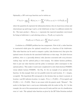
![119
Figure A·1: Hyperplanes representing the optimal Value Function
(cost framework) for the canonical Wald Problem [Wald, 1945] with hori-
zon 3 (2 sensing opportunities and a declaration) for the equal missed
detection and false alarm cost case: FA=MD.
(or approximately given by another method) is the concave hull of these hyperplanes.
The classification costs (dependent on P(H2)) give the hyperplanes their slope. The
measurement cost raises the level of the hyperplanes but does not change their slope.
The optimal value function can be written using hyperplanes called α-vectors as a
basis [Smallwood and Sondik, 1973]. The concave (convex) hull of the vectors for a
cost (reward) function gives the optimal cost-to-go value for a particular belief-state
Figure A·2: Decision-tree for the Wald Problem. This figure goes with
Fig. A·1.](https://image.slidesharecdn.com/9f5467db-22a0-4b25-9f85-d66c2d62a6f8-160910233158/85/dissertation-141-320.jpg)

![121
i.e., it is a branch of the optimal decision-tree with one less stage to go. See [Pineau
et al., 2003] or [Kaelbling et al., 1998] for more details about this formulation.
If there are |V ′
| α-vectors in the previous basis for the optimal value function, the
first step generates |U||O||V ′
| projections. The second step then generates |U||V ′
||O|
cross-
sums. Therefore, although in practice many of the vectors that are generated are domi-
nated (and therefore pruned out of the solution set), it is theoretically possible to have
|U||V ′
||O|
vectors in the value function for V , with order |X|2
|U||V ′
||O|
time-complexity.
There is an exponential growth within a single backup to the number of hyperplanes
supporting the concave (or convex) hull in the previous stage, and every one of these
new hyperplanes will become part of the problem (burden) just one stage later.
Fig. A·3 and Fig. A·4 demonstrate how the complexity of the structure of the convex
(concave) hull of the set of hyperplanes representing the optimal value function grows
with increasing dimension of the state, and this is a relatively simple example with
just 4 possible states. In general after forming the projections, the hyperplanes that are
dominated (out-performed) by other hyperplanes must be pruned out of the solution set,
and testing every hyperplane against every other hyperplane (for instance, by solving
a LP) is a time-consuming operation. Solving a single LP is of polynomial complexity,
but solving an exponentially growing number of them is exponentially complex.
Monahan provides a survey of POMDP applications and various solution tech-
niques [Monahan, 1982]. Sondik’s One-Pass Algorithm [Smallwood and Sondik, 1973]
was the first exact algorithm proposed for solving POMDPs. Michael Littman’s Wit-
ness Algorithm [Littman, 1994] is a more recent POMDP algorithm that has computa-
tional benefits over Sondik’s One-Pass Algorithm. The Witness Algorithm maintains a
set of hyperplanes to represent the optimal value function in a POMDP and then sys-
tematically generates and prunes the possible next-stage hyperplanes in performing the
DP backup (backwards recursion) operation until an optimal value function is found.](https://image.slidesharecdn.com/9f5467db-22a0-4b25-9f85-d66c2d62a6f8-160910233158/85/dissertation-143-320.jpg)
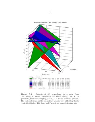
![124
The optimal value function provides (expected) cost-to-go information for every possible
belief-state and thus provides all the information necessary to select an optimal action
given a particular belief-state.
A.2 Point-Based Value Iteration
Pineau recently developed a POMDP algorithm called Point-Based Value Iteration or
PBVI that uses sampling to generate near-optimal policies [Pineau et al., 2003]. PBVI
samples belief-space and maintains a record of the hyperplane with the best value (i.e.,
the best-available action) for every belief-point (sample point). The difference between
Finite Grid Methods and PBVI is that the former only keeps track of the best value at a
belief point whereas the latter keeps track of the best hyperplane, which is enough to be
able to reconstruct an approximation of the optimal value function in the neighborhood
of the belief-point. When the belief-space can be sampled densely, Finite Grid Methods
and PBVI give very good (or perfect) solutions; however, this is intractable in high-
dimensional belief-spaces. In [Lovejoy, 1991a, Lovejoy, 1991b] a Finite Grid Method is
proposed in which a Freudenthal triangulation is used to tessellate the state-space of the
underlying MDP which gives (M +n−1)!/(M!(n−1)!) possible belief-points where n is
the number of MDP states and M is the number of samples in each dimension. In gen-
eral, the PBVI technique scales much better complexity-wise than the other techniques
for solving POMDPs and can be used to solve much larger problems near-optimally.
Assume that the set B is a finite set of belief-points for PBVI. There will be one
(optimal) α-vector computed for every belief-point in B. Using the PBVI algorithm,
the approximate value function backup operation V = ˜HV ′
can be performed with the
steps:
1.
Γu,∗
← αu,∗
(x) = R(x, u) (A.6)](https://image.slidesharecdn.com/9f5467db-22a0-4b25-9f85-d66c2d62a6f8-160910233158/85/dissertation-146-320.jpg)
![125
2.
Γu,o
← αu,o
i (x) = γ
x′∈X
T (x, u, x′
)Y(o, x′
, u)α′
i(x′
), ∀ α′
i ∈ V ′
(A.7)
3. Using the finite set of belief-points B, the cross-sum step Eq. A.4 is much simpler:
Γa
b = Γu,∗
+
o∈O
arg max
α∈Γu,o
(α · b), ∀ b ∈ B, ∀ u ∈ U (A.8)
4. The last step is to find the best action for each belief-point:
V ← arg max
Γu
b , ∀ u∈U
(Γu
b · b), ∀ b ∈ B (A.9)
As is the case with the exact value backup in Eq. A.2 - Eq. A.5, the PBVI routine
creates |U||O||V ′
| projections. However, the support for the value function V is limited
in the number of hyperplanes it can have to the size of |B| with a computational time
complexity on the order of |X||U||V ′
||O||B|. Even more importantly, the number of
hyperplanes does not “blow up” from one stage to the next as it does with the exact
backup operation. Pineau gives more details to this derivation in [Pineau et al., 2003].
A.3 Dantzig-Wolfe Decomposition and Column Generation for
LPs
In our work, we use decomposition techniques to break multi-location problems into
single location problems, coordinated by a master problem. This approach is known
as a Dantzig-Wolfe decomposition. Consider the following LP from [Bertsimas and](https://image.slidesharecdn.com/9f5467db-22a0-4b25-9f85-d66c2d62a6f8-160910233158/85/dissertation-147-320.jpg)
![126
Tsitsiklis, 1997]:
min c T
1 x1 + c T
2 x2 (A.10)
subject to D1 x1 + D2 x2 = b0
F1 x1 = b1
F2 x2 = b2
where x1 ≥ 0 and x2 ≥ 0 and Fi are linear constraints that specify a polyhedral set
of feasible points. The latter two constraints in Eq. A.10 are not coupling constraints,
but the first constraint (with the Di matrices) couples the optimal values of x1 and x2
together. Define Pi as the polyhedra describing the set of all xi such that Fi xi = bi for
i ∈ {1, 2}. We can rewrite Eq. A.10 as:
min c T
1 x1 + c T
2 x2 (A.11)
subject to D1 x1 + D2 x2 = b0
with x1 ∈ P1 and x2 ∈ P2. Now using the Resolution Theorem for Convex Polyhedra, the
variables x1 and x2 can be written in terms of a basis of extreme points and extreme
rays. Assume there are Ji extreme points and Ki extreme rays in the ith
polyhedra.
Let the vectors xj
i for j ∈ Ji represent the extreme points of the polyhedra Pi. The
vectors wk
i represent the extreme rays in the polyhedra Pi for k ∈ Ki. Obviously for
bounded polyhedra the number of extreme rays is 0. The variables xi can now be written
in the form:
xi =
j∈Ji
λj
i xj
i +
k∈Ki
θk
i wk
i](https://image.slidesharecdn.com/9f5467db-22a0-4b25-9f85-d66c2d62a6f8-160910233158/85/dissertation-148-320.jpg)
![127
with the bounds λj
i ≥ 0 ∀ i, j and θk
i ≥ 0 ∀ i, k and with a simplex constraint on the λj
i
values (we only want to allow convex combinations of the extreme points):
j∈Ji
λj
i = 1 ∀ i ∈ {1, 2}
This substitution results in the constraints:
j∈J1
λj
1
D1xj
1
1
0
+
j∈J2
λj
2
D2xj
2
0
1
+
k∈K1
θk
1
D1wk
1
0
0
+
k∈K2
θk
2
D2wk
2
0
0
=
b0
1
1
(A.12)
where the optimization variables are now in terms of λj
i and θk
i . For a general LP of the
form min cT
x subject to Ax = b, the reduced cost of variable xi is written as cT
− pT
Ai
where p is a Lagrange multiplier vector (dual variable). Therefore relative to this new
problem structure, the reduced costs for λj
i can be written as:
c T
i xj
i − [ qT ri1 ri2 ]
Dixj
i
1
0
= c T
i − qT
Di xj
i − ri1 (A.13)
and the reduced costs for θk
i are:
c T
i wk
i − [ qT ri1 ri2 ]
Diwk
i
0
0
= c T
i − qT
Di wk
i (A.14)
where the vector pT
= [ qT ri1 ri2 ] represents an augmented price vector (Lagrange
multiplier) that gives the price of violating constraints in this primal problem. The
Revised Simplex Method naturally supplies this type of pricing information as part of
its solution procedure, so no extra calculation is necessary.
Now, rather than trying to enumerate all of the reduced costs for the possibly very
large number of λj
i and θk
i variables, the best reduced cost (corresponding to whichever
non-basic variable would be most valuable to have in the basis) can be found by solving](https://image.slidesharecdn.com/9f5467db-22a0-4b25-9f85-d66c2d62a6f8-160910233158/85/dissertation-149-320.jpg)
![128
the auxiliary (related) LPs:
min c T
i − qT
Di xi (A.15)
subject to xi ∈ Pi
for each of the subproblems. Using a Column Generation procedure, if the LP solution
for subproblem i has an optimal cost that is smaller than ri1 and finite, then we have
identified an extreme point xj
i that implies the reduced cost of λj
i is negative. Therefore
a new column Dixj
i 1 0
T
for the variable λj
i is generated and added to the master
problem. If the LP solution for subproblem i is unbounded, we have identified an
extreme ray wk
i that implies the reduced cost of θk
i is negative. Therefore a new column
[ Diwk
i 0 0 ]
T
for the variable θk
i is generated and added to the master problem. If the
optimal cost corresponding to the ith
LP is no smaller than ri1 ∀ i, then an optimal
solution to the original (master) problem has been found. Clearly, there is nothing
limiting this formulation to just two subproblems; the only limit to the number of
subproblems is the available amount of computing time.
The application of a Dantzig-Wolfe Decomposition to a linear programming problem
results in the method of Column Generation. This technique can be used to solve large
systems of linear equations containing so many variables and constraints that they do
not fit inside computer memory (or in some cases can not even be enumerated). Consider
a system of equations:
min cT
x
subject to Ax = b
x ≥ 0 (A.16)
where x ∈ ℜn
, c ∈ ℜn
, b ∈ ℜm
and the matrix A is m × n with entries aij ∈ ℜ. Let Ai](https://image.slidesharecdn.com/9f5467db-22a0-4b25-9f85-d66c2d62a6f8-160910233158/85/dissertation-150-320.jpg)
![130
variables, the Cutting Plane Method can be applied to the dual problem. See [Bertsimas
and Tsitsiklis, 1997] for the full derivation of this material. Williams demonstrates how
Column Generation can be applied to a SM problem in his dissertation [Williams, 2007].
The dissertation [Tebboth, 2001] describes Dantzig-Wolfe Decompositions in more detail
including how columns can be generated in parallel to speed up the solution process.](https://image.slidesharecdn.com/9f5467db-22a0-4b25-9f85-d66c2d62a6f8-160910233158/85/dissertation-152-320.jpg)
![131
Appendix B
Documentation for column gen Simulator
The purpose of this appendix is to give a high-level overview as to the function of the
column gen simulator such that a 3rd party could pick up the program and use it for their
own simulations and/or continue to develop the code-base. The style of this appendix
is less formal than the rest of the dissertation. This program was built off of the base-
line established by Anthony R. (Tony) Cassandra while he did his dissertation work at
Brown University. His program pomdp-solve-5.3 provides a lot of the core functionality
of this simulator [Cassandra, 1999]. Nonetheless, I spent several years working with his
code base, developing and customizing it and in general had to make it work for me.
There were something like 60–80K lines of code in Tony’s program before I got to it,
and I added around 10–15K, a significant portion of the work went to understanding
and rearranging what was already there. Whereas Tony’s interests were typically in
the framework of a batch-mode execution of a POMDP solver using an infinite horizon
problem formulation, the concerns of this dissertation necessitated a program that could
execute many POMDPs in a loop (unimpeded by file-io). In addition these POMDPs
needed to have customizable parameters from one iteration to the next for such things as
variable sensor resource costs. Later on after beginning to work with “visibility groups”,
the POMDP Subproblems also needed to be able to support having a separate action-
space for each Subproblem according to the particular set of sensors that had visibility
for this Subproblem. Breaking Tony’s batch-mode program into a more modular form
able to run in a loop, learning what needed to be reinitialized or not, learning how](https://image.slidesharecdn.com/9f5467db-22a0-4b25-9f85-d66c2d62a6f8-160910233158/85/dissertation-153-320.jpg)


![136
• alpha.c/.h
• mdp.c/.h
• imm-reward.c/.h
some of which are in the same /src directory and some of which are in the /src/mdp
subdirectory. Other files were modified only on rare occasions. By convention C language
files were given suffices .c and .h and C++ language files were given suffices .cpp and
.hpp.
The following MATLAB scripts are helpful for either displaying simulation results
or debugging such things as the evolution of a belief on a decision-tree:
• DisplayPolicyGraph.m: uses MATLAB’s biograph viewer to display a color-coded
decision-tree
• ReadHyperplanesFromFile.m: helper file for DisplayPolicyGraph.m
• ReadPolicyGraphLine.m: helper file for DisplayPolicyGraph.m
• PlotLowerBoundPaperResults.m: plots the ROC curve of Fig. 2·4
• PlotValueFunction3D.m: plots the 3D value functions used in Appendix A.1
• PlotValueFunction.m: plots the 2D value functions such as in Fig. A·1
• BeliefEvolution LowerBoundPaper.m: belief-evolution test-case relevant to the
simulation results in [Casta˜n´on, 2005a]
• test case J measure J total mismatch.m: belief-evolution test-case of Fig. 2·6
• pg tree y1 y2 calcs.m: belief-evolution test-case related to Fig. A·1
B.2 Running column gen
In this project the source files are all in the column gen/src subdirectory and its subdirec-
tories. There is a limited amount of documentation in the column gen/docs subdirectory
and all of the data (as well as figures, some MATLAB scripts etc. . . ) are stored in the](https://image.slidesharecdn.com/9f5467db-22a0-4b25-9f85-d66c2d62a6f8-160910233158/85/dissertation-158-320.jpg)

![139
e.g. “// =>obs” to indicate that obs was being returned by reference or by pointer. I
made extensive use of dynamic memory allocation, but stuck with Tony’s version of the
malloc calls: XMALLOC(), XFREE() and so on. When I had a dynamically allocated
variable, that variable was passed using pointer notation (not array notation), however
I attempted to indicate the sizes of all dynamically allocated structures using comments
of the form e.g. “pArray/*[2][3]*/” to indicate that despite the fact that “pArray” may
have been a pointer of type “double **”, it had been allocated to store a matrix with
2 rows and 3 columns. This type of notation helped me out significantly in not getting
confused while changing contexts between what I was working on.
I wrote this program assuming that one vehicle would have multiple sensors under
its direction and that eventually the sensors would be constrained to moving together
(and only looking at things within a certain range of the vehicle). This is still work
in progress. Currently there are no constraints on what locations/objects a vehicle’s
sensors can look at (other than the 0/1 type visibility constraints). Whereas I would
have preferred to set a sensor-centric limit on the locations each sensor can look at (like
in the CVehicle (aka sensor-platform) class), the ColumnGen() planning sub-routine was
written well before knowing it would be used in this way. Therefore it was easier to store
information in the TaskList[] array (an output of and also an input to the ColumnGen()
function) to specify which sensors can look at which locations. The TaskList[] global
array-variable has location-by-location information stored in it during the ColumnGen()
function’s execution (more to follow). At this point in time, the CVehicle class in the
simulator is just a container for all the sensors in the program, and no code concerning
the positions of sensors (or locations of cells) is active/useful. The global array TaskList[]
ought to be a local variable, an argument to the ColumnGen() function, and be passed
down through the call-chain. This would fix several different issues, but is still work
in progress. As is there is just one vehicle and there is no relationship/no constraints](https://image.slidesharecdn.com/9f5467db-22a0-4b25-9f85-d66c2d62a6f8-160910233158/85/dissertation-161-320.jpg)
![140
on the activities of the sensors which it holds. The only issue is that the simulation
calls pVehicle->update() once per update cycle (were pVehicle is actually an Standard
Template Library (STL) iterator), which causes one sensing task in the vehicle’s task-
list (CVehicle::m taskList) to be undertaken. A more realistic account of time might
entail updating each “vehicle” once for each sensor it contains, or else creating multiple
vehicles that are each limited to containing one sensor. Again, this is work in progress.
The vehicles maintain vector-resource information and vector-constraints on expected
resource expenditure and handle multiple tasks for multiple sensors appropriately. For
better or worse they process the tasks for multiple sensors in serial fashion however; if
it mattered, this could easily be changed. Another reason that the TaskList[] variable is
suboptimal is because it is very similar in name to the CVehicle::m taskList variable, and
the two variables have no relation to each other. Additionally, if the Column Generation
code was not dependent on the TaskList variable, then it would be possible to run
multiple CSimulator objects in parallel (i.e. to support multiple concurrent simulations).
I attempt to more or less exhaustively assert every condition I can at the beginning
of function-calls, and elsewhere as well. These assertions have the form ‘Assert(x >0,
“Something is broken, x <= 0”);’. The string in the second argument of the “Assert()”
function is displayed when the assertion fails (and the program terminates at that point).
While there were many false alarms that had to be dealt with in working with these
assertions (getting them straight/self-consistent), they were nonetheless extremely useful
in assuring a consistent+valid state of the program. In addition, this assertion function
(at least under Linux) gives a file-name and line-number when it fails, which helps in
the debug process quite a bit. In developing code, the sooner one can detect a problem
after it occurs, the easier it is to handle and fix. So as not to slow the program down
after it has been debugged, the “Assert()” function can be “#define’d” away to a null-
function or else a pre-processor directive can be used to comment out the body of the](https://image.slidesharecdn.com/9f5467db-22a0-4b25-9f85-d66c2d62a6f8-160910233158/85/dissertation-162-320.jpg)
![141
function. The one issue is that any assertion of the form “Assert(0,””);” should not
really be an assertion, it should be an “exit(-1);”-type statement. Actually Tony wrote
an Abort() function that provides a parameter for a textual description of the error
condition, I should have been using that function instead of “Assert(0,””);”. After the
program is stable (and I believe it is at least fairly stable + well-debugged as is), the
Assert() statements can be turned off but the Abort() and exit()-like statements should
remain. At that point it would make sense to start turning on compiler optimizations
and tuning the algorithm for speed using performance profiling.
I also #define’d a series of “VALID [something]()” type macros in global.h that are
used to test the validity of the range of some variable in a consistent fashion. Consistency
is everything. These macros also reveal a lot of information about the conventions used
in this program and so are a very good means of studying how the various variables are
used and what types of values for e.g. states or observations or sensor indices etc. . . are
allowable.
As much as possible, whenever I changed Tony’s code, I attempted to document
those changes with comments of the form /* Darin’s Modification [date] – description
*/. This worked well when I was making precise changes to his code, but was more messy
at the interface of what my code and his code were doing. I think at some point with
the column gen.c and pomdp solve 5 3.c files, I quit bothering; those files are basically
of my authorship now.
There are numerous different types of “0” in programming, and I tried to disam-
biguate between them to make the code clearer. So first and foremost I used “0” for
ints (integers) and “0.0” for floats and doubles. And while “NULL” equates to a “0”
for string and pointer comparisons, I used “NULL” anyway for clarity of exhibition.
The same goes for using “FALSE” and “TRUE” in C code (or “false” and “true” in
C++ code) instead of merely 0 and 1.](https://image.slidesharecdn.com/9f5467db-22a0-4b25-9f85-d66c2d62a6f8-160910233158/85/dissertation-163-320.jpg)

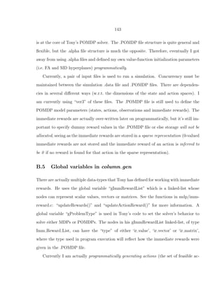
![144
tions) based on the contents of the .POMDP file as well. I use the actions defined in the
.POMDP to specify a template for the actions a sensor can support. (This is a departure
from Tony’s paradigm). The (primary) global variables gNumStates, gNumActions and
gNumObservations are set as the .POMDP file is read in. This happens very early in the
program starting from the initPomdpSolve() function. (I broke the initialization code of
pomdp-solve-5.3 into pieces however). After reading in the .POMDP file, my simulation
data input file, of type .data, is read in and then, according to the instructions in my
file, sensors (sensor actions) are instantiated based on the sensor-action templates in the
.POMDP file. Therefore I modify the value of gNumActions on the fly. I read in and
parse my simulation parameters in the function ReadSimulationData() in column gen.c.
(More to follow).
The following is a list of most of the significant global variables that were used within
the original pomdp-solve-5.3 program (and are mostly still in use now):
• Matrix *pomdp P/*[TotalSensorActions]*/: POMDP model transition prob.
• Matrix *pomdp R/*[TotalSensorActions]*/: POMDP model observation prob.
• Matrix pomdp Q: POMDP model immediate values for state-action pairs
• I Matrix *IP: temporary matrix of transition prob. (used while reading .POMDP file)
• I Matrix *IR: temporary matrix of observation prob. (used while reading .POMDP file)
• int gNumStates: number of states in the POMDP model
• int gNumActions: number of actions in the POMDP model (I rewrite this value)
• int gNumObservations: number of observations in the POMDP model
• int *gNumPossibleObservations/*[gNumActions]*/: mainly used to ensure that every
action generates at least one observation
• int **gObservationPossible/*[gNumActions][gNumObservations]*/: controls which branches
of the decision-tree are so improbable as to not be worth “walking” (to include in
expected cost calculations), also determines the projections that are created in the
POMDP backup operation
• Imm Reward List gImmRewardList: linked-list that stores immediate reward values
• Problem Type gProblemType: should be ‘POMDP problem type’ for our case
• double gDiscount: should be 1.0 for a finite-horizon POMDP
• Value Type gValueType: should be ‘REWARD value type’, the cost-based formulation](https://image.slidesharecdn.com/9f5467db-22a0-4b25-9f85-d66c2d62a6f8-160910233158/85/dissertation-166-320.jpg)
![145
is broken
• double gMinimumImmediateReward: equal to the most costly measurement reward,
jump-starts Value Iteration by establishing a lower bound on the costs
• double *gInitialBelief: not part of the active code-base, I specify prior probabilities in
my own input (.data) file
Tony’s code defined the sparse matrices P (transition probabilities), R (observation
probabilities) and Q (immediate rewards), which was all well and fine when just one
POMDP was being solved, but after starting to work with visibility groups, this was
no longer the case. Therefore I did a project-wide search+replace and renamed these
variables pomdp P[], pomdp R[] and pomdp Q, but far more significantly, I introduced
arguments to a large portion of his hundreds of functions (the entire code-base of 60–80K
lines), so that the program is not forced to refer to pomdp P[], pomdp R[] and pomdp Q.
I introduce a structure that I call “sensorPayload” that contains these values, as well
as a customized version of immRewardList, actionNames[] etc. . . that allows POMDPs
with different numbers of actions (or different encodings for actions) to be solved by his
code. I should have called “sensorPayload”, “sensorConfiguration”, the name is a bit of
a misnomer. At any rate I define one such structure (that represents all the POMDP
problem parameters) and pass it in to Tony’s solvePomdp() function to compute a
solution. This is the largest single change I made to his program, and it took about a
month to do this, create the programmatically defined actions and debug the results.
I also had to break certain portions of the code that was in solvePomdp() into pieces
and moved some code to per-solution-call setup and shutdown code that comes before or
after the call to the solver respectively. I also changed the initialization of the Finite Grid
code so that the belief-point grid is generated once per program instead of once per call
to the POMDP solver. One last significant change that I made to the pomdp-solve-5.3
code is that I updated it to use the lp solve-5.5.0.13 solver instead of the far older and far
inferior lp solve-2.x solver. The newer version of the program is in a whole separate class](https://image.slidesharecdn.com/9f5467db-22a0-4b25-9f85-d66c2d62a6f8-160910233158/85/dissertation-167-320.jpg)
![146
of program than the older. Nevertheless, this change only affects the Witness Algorithm
code, which I stopped using because it was still too slow. We decided that because
the Finite Grid method is already an approximate technique, solving LP’s to prune
hyperplanes is rather silly, so we use simpler pruning methods. For all the advances
to lp solve, I gather it still only runs about 5% as fast as cplex. Despite the fact that
lp solve-5.5.0.13 is not currently being used to solve POMDPs, it is still useful to have
the LP solver in the program when it comes to iteratively solving the LPs used in Column
Generation.
I have done a major modification to the way pomdp P[], pomdp R[] and pomdp Q
are created from the temporary matrices IP[] and IR[], see the function ReadSimulation-
Data() for details. In terms of how the matrices pomdp P[], pomdp R[] and pomdp Q
are accessed in this program, take a look at the function showProblemMatrices() that
shows typical usage. This is a debug function that prints the values of each of these ma-
trices to stdout. Tony has created numerous such debug functions that are very useful
for printing debug output such as for hyperplanes, policy-graphs etc. . . to the console.
Here is a list of some of the more important global variables and arrays I have added
to this program:
• int NumTargets: number of locations
• int GridSizeX, GridSizeY: are in use but nearly useless until vehicles (sensors) have
locality constraints
• int NumTargetTypes: number of object types (including one for ‘empty’)
• int NumDecisions: number of decision/declaration hyperplanes read in from .data input
file
• int NumSensorTypes: number of templates for sensors, .data and .POMDP file values
must jive
• int NumTargetGroups: the number of groups of targets with distinct a priori probabili-
ties
• int NumVisibilityGroups: determined by counting how many different classes of visibility
the prior probabilities are divided into in the .data file
• unsigned int *VisibilityGroups/*[NumTargets]*/: defined with the maximum possible](https://image.slidesharecdn.com/9f5467db-22a0-4b25-9f85-d66c2d62a6f8-160910233158/85/dissertation-168-320.jpg)
![147
but only using NumVisibilityGroups elements
• Target *TaskList/*[MAX NUM TARGETS]*/: per location solution data after Colum-
nGen() is executed, also specifies the inputs for prior probabilities and sensor visibilities
to the ColumnGen() function
• int TotalSensorCount: number of instantiations of sensors (which are programmatically
generated from .POMDP file)
• int DistinctSensorActions: the number of (parsimonious) actions specified in the POMDP file
• int TotalSensorActions: the number of actions across all (programmatically generated)
sensors
• int *ParsimSensorStartIndex/*[NumSensorTypes]*/: I want to be able to find the index
of the jth mode of sensor i when all of the sensor modes are embedded together in
one long list (stored in a sparse format) where there are a different number of possible
modes (sensor actions) depending on which sensor is being used. Therefore I’m using
the array ParsimSensorStartIndex[] to store the index of the first mode (j = 0) for
each of the NumSensorTypes sensors. (This is very similar to how for sparse matrices
the beginning row indices are stored in the Matrix structure as row start[row i]). I’m
prepending “parsim” => parsimonious to indicate that each (sensor,mode) combination
has a unique action index associated with it in this array. Therefore a vehicle which has
multiple instances of the same type of sensor in its sensorPayload structure will have
each of its equivalent sensors’ modes be mapped to the same set of action indices when
referring to the array ParsimSensorStartIndex[]. I’m using this scheme so that I don’t
have to store action names and the relative costs for the sensor modes redundantly for
each of the duplicate/cloned/equivalent sensors that each vehicle may have. Each of the
sensorPayload structures contains a similar array called “sensorStartIndex[]” which has
the starting indices for each of the sensors contained in that sensor payload. In general
each sensorPayload structure has a distinct/independent sparse encoding for its actions
• int *SensorStartIndex/*[TotalSensorCount]*/: sparse mapping/encoding for the first
action in a joint list of actions (across all sensors) that corresponds to a sensor
• int *SensorTypes/*[TotalSensorCount]*/: type of each programmatically generated sen-
sor where the types are defined by the actions in the .POMDP file
• int *ActionToSensorMap/*[TotalSensorActions]*/: index of the (programmatically gen-
erated) sensor that does a (programmatically generated) action
• int *NumActionsPerSensorType/*[NumSensorTypes]*/: number of actions that each
sensor in the parsimonious list (from .POMDP file) can do
• char **actionNames/*[TotalSensorActions+NumDecisions][40]*/: names for (program-
matically defined) actions stored in a sparse format (i.e. all sensors confounded with a](https://image.slidesharecdn.com/9f5467db-22a0-4b25-9f85-d66c2d62a6f8-160910233158/85/dissertation-169-320.jpg)
![148
variable number of “actionName” strings per sensor)
• char **stateNames/*[NumTargetTypes][40]*/: ragged array of strings for state names
• char **observationNames: ragged array of strings for observation names
• int *stateList/*[NumTargetTypes]*/: deprecated, used when I had a terminal capture
state instead of ‘wait’ actions
• double *SensorTimeCost/*[TotalSensorActions]*/: the relative cost of each sensor mode
as specified in the .data file
• UINT32 TraceFlags: 32-bit unsigned integer that stores bitwise flags used for filtering
program output
The arrays SensorStartIndex[], SensorTypes[], ActionToSensorMap[] and actionNames[]
are all sparsely-defined. The arrays NumActionsPerSensorType[] and ParsimSensorStartIn-
dex[] are defined w.r.t. the number of classes of sensor that the actions in .POMDP are
divided into. (The .POMDP file lists all the possible actions in one long list, my .data file
is responsible for associating one action or another with a class of sensor, i.e. a sensor
template. Once the number of actions per sensor template is established, it is possible
to specify how many sensors of each type are desired within a simulation).
The input files searchAndExploit ver3.POMDP and searchAndExploit ver3.data are
a pair as are lwrBoundPaper ver3.POMDP and lwrBoundPaper ver3.data. These files
have a lot of parameters between them that need to be set correctly in order for these
sparse arrays to function correctly. There are some comments at the top of my *.data
files that describe how those files are laid out and the documentation Tony provides for
his program remains in effect for the .POMDP files. First and foremost, great care needs
to be taken to specify parameters lists that are w.r.t. a parsimonious action list if the
parsimonious values are required or w.r.t. the expanded/programmatically generated
list of actions if that is required. (If there are 3 sensors that each support ‘mode1’ and
this mode has identical statistics for all 3 sensors, then ‘mode1’ would appear once in a
“parsimonious” list of actions but 3 times in the expanded/programmatically generated
list of actions, which generates 3 actions for the POMDP solver based off of the prototype](https://image.slidesharecdn.com/9f5467db-22a0-4b25-9f85-d66c2d62a6f8-160910233158/85/dissertation-170-320.jpg)
![149
‘mode1’ specified in the .POMDP file). In the .data files for my simulation parameters,
I give a comment line above each row of parameter values that serves to document what
that row is for and how many parameters should be there. My input files understand %’s
at the beginning of lines and at the end as well. I specify resources and initial lambda
values w.r.t. the parsimonious action list and then replicate these values as appropriate
when sensors are instantiated from the templates defined in the .POMDP file; currently
if there are multiple sensors of the same type in a simulation, then they must share the
same values for initial sensor resources and initial lambdas (used to create an initial
basis for Column Generation).
As a brief overview, imagine the .POMDP file has the actions ‘wait 0’, ‘search 0’,
‘mode1 0’, ‘wait 1’, ‘mode1 1’, ‘mode2 1’, which serves to indicate that there are 2 classes
of sensor, that the first sensor has a ‘search’ and a ‘mode1’ action, and that the second
sensor has a ‘mode1’ and a ‘mode2’ action. This is the parsimonious action list. (I also
described it as a “Distinct” action list). (The tags (suffixes) for which sensor each action
belongs to are programmatically over-written when the actionNames[] array is created
for the expanded set of actions). The .data file might have a line that instantiates 2
of the first type of sensor and 1 of the latter: ‘3 0 0 1’ (this is the 3rd non-comment
line in the file). SensorTypes[] takes on the value of the last 3 params on this line. The
indices specify that 3 sensors of types 0, 0 and 1 will be used in the simulator. (All
indices in the program are always 0-based, except for certain lp solve-5.5 function calls).
This specification would cause a list of actions to be defined (and the value of gNumAc-
tions to be modified) such that the (non-parsimonious) actions are: ‘wait 0’, ‘search 0’,
‘mode1 0’, ‘wait 1’, ‘search 1’, ‘mode1 1’, ‘wait 2’, ‘mode1 2’, ‘mode2 2’ (this list would
correspond to the first 9 entries in the actionNames[] array. (The actionNames[] array
stores the names of the decision (aka declaration or classification) hyperplanes after this
list of 9 action names). In this example, TotalNumSensors = 3, TotalSensorActions = 9,](https://image.slidesharecdn.com/9f5467db-22a0-4b25-9f85-d66c2d62a6f8-160910233158/85/dissertation-171-320.jpg)
![150
DistinctSensorActions = 6, and SensorStartIndex[] = [0 3 6]. ActionToSensorMap[] =
[0 0 0 1 1 1 2 2 2].
The simulator uses 3 separate seeds for random number generation that are used for
different purposes. The use of multiple seeds allows concurrency to be maintained across
simulation runs. The seed “gCellSeed” controls the states (the types) of each location
(cell) in a simulation run. The seed “gMeasurementSeed” controls how the trajectory of
random observations evolves. The seed “gStrategySeed” is mainly used for the methods
of RH control that employ randomization (i.e. “randomly choose a pure strategy on
a per location basis with a distribution given by the measure weights”). By resetting
the value of gCellSeed after every series of 100 Monte Carlo simulation runs (but after
changing the resource levels, MD to FA ratios, horizon etc. . . ) it was possible to ensure
that each batch of 100 simulations used the same trajectory of cell (location) states, but
that these states evolved randomly from one simulation run to the next.
Two enumerated types are worthy of mention. The first is used for controlling the
display of tracing information (i.e. logging of debug information to stdout or a file) in a
programmatically controllable fashion (rather than having all program output be fixed).
I created my own version of a printf() function, called myprintf(), and added another
parameter (a bitwise variable of boolean flags) that is passed in to each myprintf()
function call. A global variable called “TraceFlags” implements the other half of the
lock+key mechanism. When the global variable TraceFlags has matching bits with one
of the descriptive codes given to the myprintf() function, output is generated in the
log-file, see Section B.3. Therefore these trace-codes act as filters and control how much
if any debug information is stored. Unless a very specific aspect of the program is being
tested, then all of the lower-level trace-codes cause output to be generated so fast, so
verbosely, that the program can not run while they are active; they are only of use for
testing a single function call or chain of low-level function calls. I attempted to do this](https://image.slidesharecdn.com/9f5467db-22a0-4b25-9f85-d66c2d62a6f8-160910233158/85/dissertation-172-320.jpg)

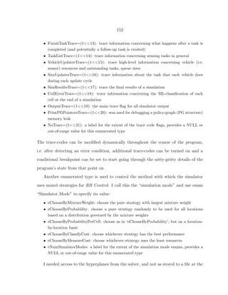
![153
end of the program (after using the “save-all” pomdp-solve-5.3 command-line switch)
(this had been the status quo), but in memory during the life-cycle of the program,
so I had to dig into the solver code. These hyperplanes are stored in next alpha list
and prev alpha list in the solvePomdp() function that Tony wrote. I added a level
of indirection that allowed me to use the pointer mechanism to output these lists
from solvePomdp(). I only ever bothered to get the hyperplanes from the last stage
and penultimate stage however. I needed the latter because the former points into
the latter. Therefore I had to wait to destroy the penultimate-stage hyperplanes un-
til I was done tracing the policy-graphs to back out the measurement versus clas-
sification costs. Policy-graphs are stored in a structure that holds all the data for
one stage, see some of Tony’s debug/output routines in pg.c for more info. In or-
der to represent strategies, I created a 3D dynamically allocated array: “PG ***
strategyTree/*[TotalSensorCount+1][NumVisibilityGroups][horizon]*/”. An individual
decision-tree could be represented as: “PG * policyGraph/*[horizon]*/”, however when
working with visibility groups, different subsets of sensors will in general have distinct
POMDP solutions with different decision-trees, hence the need for the 2nd dimension
in this structure. The 3rd dimension with size [TotalSensorCount+1] is needed to rep-
resent one whole mixed strategy (as a mixture of TotalSensorCount+1 pure strategies).
At points in the code I referred to one of the component pure strategies as a “PG **
policy graph group/*[NumVisibilityGroups][horizon]*/”. Hyperplanes are stored as a
linked-list of “AlphaList” nodes and the ids of the nodes correspond to the ids of the
hyperplanes. The hyperplane coefficients themselves are stored in the member “alpha[]”
of AlphaList. One other important point is that for whatever reason, Tony left the root
node in a list of hyperplanes as a dummy/header node (stores summary statistics not
hyperplanes) and then all the actual data follows after that in the linked list. He also
has 2 separate ways of accessing immediate rewards (the pomdp Q sparse matrix and](https://image.slidesharecdn.com/9f5467db-22a0-4b25-9f85-d66c2d62a6f8-160910233158/85/dissertation-175-320.jpg)
![154
the gImmRewardList linked-list). In addition he uses the global variable gCurAlphaVec-
tor as an array (basically a vector) that points into his linked-lists of hyperplanes. So
he maintains hyperplanes both as a linked-list of nodes and also indexes them with a
vector/array as the situation warrants.
After the call to solvePomdp() and after tracing the decision-trees, I store per-task
information on classification costs and measurement costs in the global array TaskList[].
This methodology with this global array variable is suboptimal because it prevents mul-
tiple simulators from being able to run in parallel, and I had the intention of modifying
this code to make it more object-oriented; this is work in progress, but at least it works
as is.
The routine that runs the Column Generation algorithm in the simulator is:
double ColumnGen(
const SensorPayload *sensorPayloadList/*[NumVisibilityGroups]*/,
PomdpSolveParams param,
PG **policy graph group/*[NumVisibilityGroups][horizon]*/,
double **lambdaOfStrategy/*[MAX COLUMNS+1][TotalSensorCount]*/,
const double *R/*[TotalSensorCount]*/,
double *initLambda/*[TotalSensorCount]*/,
PG ***strategyTree/*[TotalSensorCount+1][NumVisibilityGroups][horizon]*/,
int *strategyToColumnMap/*[TotalSensorCount+1]*/,
int *pColumnsInSolution,
REAL *pSolution/*[TotalSensorCount+1]*/,
double *J classify perStrategy/*[TotalSensorCount+1]*/,
double **J measure perStrategy/*[TotalSensorCount+1][TotalSensorCount]*/)
The return value is the optimal total (measurement+classification) cost of the LP at the
end of Column Generation. Occasionally, it is possible that a degenerate mixed strategy](https://image.slidesharecdn.com/9f5467db-22a0-4b25-9f85-d66c2d62a6f8-160910233158/85/dissertation-176-320.jpg)
![155
is created (less pure strategies in the LP’s basis than anticipated) in which case I still
deem the result the “optimal” cost. However, when lp solve-5.5 solves the LP for the
Column Generation Master Problem, if it does not return back a successful error flag
(that the optimal solution was found or that the LP was solved in the pre-solve step),
then the program Assert’s false and terminates. The arguments to ColumnGen() have
the following purposes:
• const SensorPayload *sensorPayloadList/*[NumVisibilityGroups]*/: describes the POMDP
problem parameters for each subset of sensors
• PomdpSolveParams param: Tony’s main structure that I pass on to his solvePomdp()
routine
• PG **policy graph group/*[NumVisibilityGroups][horizon]*/: temporary storage that I
use repeatedly
• double **lambdaOfStrategy/*[MAX COLUMNS+1][TotalSensorCount]*/: stores the tra-
jectory of lambda values
• const double *R/*[TotalSensorCount]*/: the available resources for each sensor
• double *initLambda/*[TotalSensorCount]*/: the initial lambda values used to start Col-
umn Generation
• PG ***strategyTree/*[TotalSensorCount+1][NumVisibilityGroups][horizon]*/: pure strate-
gies output from Column Generation
• int *strategyToColumnMap/*[TotalSensorCount+1]*/: mapping that describes the ac-
tive columns/the columns with support at the end of the Column Generation process
• int *pColumnsInSolution: value returned by pointer for the number of columns (out of
a total of (MAX COLUMNS+1)) that were generated in Column Generation
• REAL *pSolution/*[TotalSensorCount+1]*/: the mixture weights of each strategy with
support
• double *J classify perStrategy/*[TotalSensorCount+1]*/: the classification cost (across
all N locations) for each strategy
• double **J measure perStrategy/*[TotalSensorCount+1][TotalSensorCount]*/: the mea-
surement (sensor resource) cost (across all N locations) for each strategy
For simplicity, in the Column Generation process storage was allocated for up to (MAX COLUMNS+1
and then only some of that memory was actually used as reported by the value of
(*pColumnsInSolution). The array strategyToColumnMap[] is a mapping for the pure](https://image.slidesharecdn.com/9f5467db-22a0-4b25-9f85-d66c2d62a6f8-160910233158/85/dissertation-177-320.jpg)
![156
strategies indexed as [0,. . . ,TotalSensorCount+1] back to the range [0,. . . ,MAX COLUMNS+1]
and specifies the (TotalSensorCount+1) elements out of (MAX COLUMNS+1) that are
part of the solution. For instance lambdaOfStrategy[strategyToColumnMap[i]][j] would
give the jth
Lagrange multiplier of the ith
strategy.
In some situations it is possible for the ColumnGen() function to fail to find a non-
trivial Column Generation solution (by failing to establish an initial basis of linearly-
independent columns for the LP), or to otherwise give back results where e.g. just one
pure strategy is used when there are 2 sensors (so one would expect 3 pure strategies in
the solution). If less than TotalSensorCount+1 pure strategies have support, then one or
more elements of strategyToColumnMap[] are set to -1. These circumstances typically
arise at the end of a simulation when few resources are remaining and either no modes
are feasible for a sensor given its resource constraints, or else the cost versus benefit of
using a sensor mode weighs against the use of any resources in a particular situation.
This can happen for instance if all of the cell information states (the probability vectors
for each of the locations) are already very lopsided (low entropy), and there is not much
uncertainty left in the states of any of the locations.
When some sensors effectively have no more resources, but other sensors are still
useful, it would be ideal to eliminate the use of the resource-less sensors from consid-
eration in the ColumnGen() function and to reduce the size of the POMDPs that are
solved in the solvePomdp() algorithm. Currently this is work in progress. The untoward
result of not doing this pruning operation is that many more columns can be generated
while running Column Generation and looking for precisely the right value of Lagrange
multiplier that will satisfy a nearly infeasible constraint. While this does not crash the
program, it does waste some time. However if presolving is used with the lp-solve 5.5
solver and constraints are eliminated from the Column Generation LP, it is important
to make sure to access the solution (Lagrange multipliers in the solution) in the right](https://image.slidesharecdn.com/9f5467db-22a0-4b25-9f85-d66c2d62a6f8-160910233158/85/dissertation-178-320.jpg)
![157
way. For example, the lp-solve 5.5 functions get Nrows() and get Ncolumns() return
back the number of rows and columns of the presolved model (after rows or columns
are eliminated). The functions get Norig rows() and get Norig columns() return back
the number of rows and columns in the LP before presolving. In order to know solution
variables relative to the original enumeration for variables and constraints, the function
get var primalresult() must be used. Currently my code only supports a static indexing
of rows and columns and does not perform presolving operations that eliminate rows or
columns. See the function CreateLP() in column gen.c for the relevant section of code.
(However, when I modified Tony’s pomdp-solve-5.3 code to make use of lp-solve 5.5, I
did enable presolving w.r.t. solving the LPs that prune hyperplanes. See the function
LP loadLpSolveLP() in his file lp-interface.c for more details). Eliminating sensors from
consideration that are not useful and that slow down Column Generation is one of the
two or three most important things that can be done to improve this program.
B.6 Simulator Design
Fig. B·1 shows how the column gen program’s startup process. The function parseCmd-
LineAndCfgFile() is from pomdp-solve-5.3 and is responsible for generating the Pomdp-
SolveParams structure that contains all of the parameters for the POMDP solver except
for the matrices pomdp P[], pomdp R[] and pomdp Q. After a CSimulator object is
created, I call initPomdpSolve() and the .POMDP file parameters are read in from
file. My simulation parameters are parsed in the function ReadSimulationData() and
the matrices pomdp P[], pomdp R[] and pomdp Q are created at this time (from a
set of intermediary/temporary, dense matrices that were created during the execution
of initPomdpSolve()), and the linked-list gImmRewardList is created. At this time I
create a sensorPayload structure that represents a custom set of solution variables for
every subset of sensor visibilities that is of interest. The visibility groups of interest](https://image.slidesharecdn.com/9f5467db-22a0-4b25-9f85-d66c2d62a6f8-160910233158/85/dissertation-179-320.jpg)
![158
are determined after reading in the groups of prior probabilities from the .data file and
determining how many distinct classes of visibility these priors are arranged into. As
discussed in Ch. 3, prior probabilities for targets and sensor-target visibility is specified
in the .data file (the last lines in the file) for example as:
• 10 01 0.10 0.20 0.60 0.10 % 10 targets w/ prior π1 can be seen by sensor 0
• 90 11 0.02 0.06 0.12 0.80 % 90 targets w/ prior π2 can jointly be seen by sensors 0+1
In this example π1 = [0.100.200.600.10]T
and π2 = [0.020.060.120.80]T
and the position
of the 0th
sensor is on the right-hand side of the bitmask. The total number of targets
that these target groups add up to needs to be consistent with the parameters given in
the first line of the .data file (NumTargets = NumCellsX * NumCellsY). Once again,
until there is motion planning and locality constraints, the physical dimensions of the
grid (the layout of the locations) have no meaning.
The following is a pseudo-code for the operation of ColumnGen():
• set all Lagrange multipliers to ∞
• call ComputeResourceUsage() to compute classification cost for do-nothing strategy
• for i=1 to TotalSensorCount (i=0 is the do-nothing strategy):
– set Lagrange multipliers to initialize ith column
– call ComputeResourceUsage() to compute costs for strategy i
– add pure strategy from solvePomdp() to strategy tree
– store objective function coefficients and resource usage data in variables for LP
tableau
• if initialization was not successful, break out of function
• call CreateLP() using variables stored for LP tableau
• while Column Generation not converged:
– call SolveLP()
– store Lagrange multipliers from the solution of the LP
– call ComputeResourceUsage() with current Lagrange multiplier vector
– add pure strategy from solvePomdp() to strategy tree
– store objective function coefficients and resource usage data in variables for LP
tableau](https://image.slidesharecdn.com/9f5467db-22a0-4b25-9f85-d66c2d62a6f8-160910233158/85/dissertation-180-320.jpg)
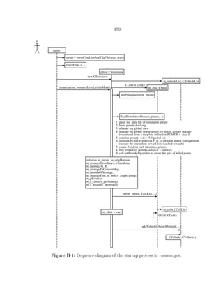
![160
– create and append new column with variables for LP tableau
• find the strategies in the final LP tableau with support
• call ComputeResourceUsage() for each final pure strategy with support and (this time)
record per-task solution data
• output solution data to console or to file as determined by the trace flag settings
where the function ComputeResourceUsage() has the following form:
• for i = 0 to TotalSensorCount-1:
– for v = 0 to NumVisibilityGroups-1:
∗ if vth sensorPayload contains ith sensor then update sensor payload’s Q and
immRewardList structures for sensor price according to current lambda vector,
convert to reward formulation
• update master list (pomdp Q and gImmRewardList) for the new sensor prices, convert
to reward formulation
• for j = 0 to NumVisibilityGroups-1:
– get pointer to jth sensorPayload structure
– call initPomdpSolveSolution(), per-solver-call code I specialized out of Tony’s init-
PomdpSolve() function
– call solvePomdp() using POMDP model in jth sensorPayload structure
– call convertActions() to convert the results of solvePomdp() which are relative to
the action list stored in jth sensorPayload structure, to the global, joint-action list
– trace hyperplane info or strategy (policy-graph) (or not) according to trace flag
settings
– initialize measurement-cost vector J measure[] to 0.0
– initialize scalar variable J classify to 0.0
– for i = 0 to NumTargets-1:
∗ call computeExpectedCosts()
· call findInitialHyperplane() to find the best hyperplane (action) for Sub-
problem i
· call walkPolicyGraph() to break apart classification and measurement
costs for Subproblem i
· accumulate the measurement cost of Subproblem i in measurement-cost
vector J measure[]
∗ accumulate the classification cost of Subproblem i in the scalar variable J classify](https://image.slidesharecdn.com/9f5467db-22a0-4b25-9f85-d66c2d62a6f8-160910233158/85/dissertation-182-320.jpg)
![161
∗ store per-Subproblem solution info in TaskList[] structure, convert from reward
formulation
– call cleanUpPomdpSolveSolution() to do per-solver-call cleanup work
Fig. B·2 shows how/when the C++ simulator makes use of the ColumnGen() al-
gorithm for computing sensor plans. The general algorithm consists of establishing a
count-down timer that re-plans when either a) a number of tasks has been done that
is equal to some multiple of the number of targets (Subproblems), or b) there are no
more outstanding tasks to do. Fig. B·3 gives an overview of the C++ simulator’s oper-
ation as it concerns RH Control and the execution of sensing tasks. The algorithm is
fairly straight-forward and has relatively low computational complexity (and program-
ming complexity). The one issue worthy of discussion is how the simulator maintains
an expected resource budget for each sensor. The code keeps track of the sensor re-
sources available as well as the expected resource cost for all outstanding (scheduled)
tasks. The simulator does not try to schedule any tasks beyond the point where: sensor
resources available - (expected resource cost for all scheduled tasks + cost of new task)
< 0. Instead, tasks are stored on two separate prioritized lists (queues): a list of tasks
that are definitely scheduled to be executed “m taskList” and then a list of tasks that
are conditionally executed if resources are left over after executing all the tasks from
m taskList. The latter list of potentially executed tasks is called “m delayedTaskList”.
delayed =>potential tasks. (If resource utilization is less than expected, extra tasks from
m delayedTaskList are scheduled). Tasks are added onto these two lists according to an
entropy-gain value that is used to sort/prioritize tasks. A new task with high priority
can pop lower value task(s) off of m taskList and push them onto m delayedTaskList.
(However, currently I don’t think that one high value task can pop off two lower value
ones. . . ). Tasks that can not be scheduled within the expected resource constraints are
simply ignored.](https://image.slidesharecdn.com/9f5467db-22a0-4b25-9f85-d66c2d62a6f8-160910233158/85/dissertation-183-320.jpg)
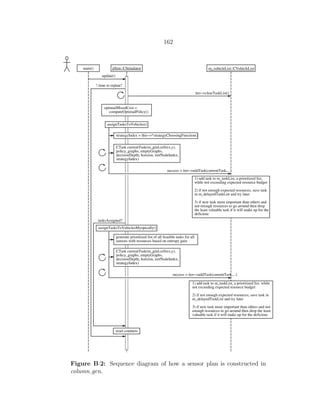
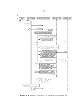

![165
on the nodes of the decision-tree (PG nodes) while walking the decision-trees for each
pure strategy. The variable J measure downstream[] keeps track of this information.
The objective was to not just keep track of the immediate deterministic resource costs
(which is trivial), or all of the resource costs until the end of the horizon (which is
what the walkPolicyGraph() function does), but to keep track of expected resource
expenditures over intermediate horizons as well. This allows the simulator to follow
a plan that in expectation will execute e.g. two sensing tasks per location when the
Column Generation sensing plan was computed with a horizon of 4 sensing actions per
location.](https://image.slidesharecdn.com/9f5467db-22a0-4b25-9f85-d66c2d62a6f8-160910233158/85/dissertation-187-320.jpg)
![166
CSimulator
− CGrid m_grid;
− CVehicleList m_vehicleList;
− int m_updateCount;
− PomdpSolveParams m_param;
− ColumnGenParams m_simParams;
− int m_origHorizon;
− int m_resourceLevelIndex;
− SensorPayload * m_sensorPayloadList/*[NumVisibilityGroups]*/;
− double *m_lambda/*[TotalSensorCount]*/;
− double *m_R/*[TotalSensorCount]*/;
− PG ** m_policy_graph_group/*[NumVisibilityGroups][horizon]*/;
− PG *** m_strategyTree/*[TotalSensorCount+1][NumVisibilityGroups][horizon]*/;
− REAL * m_pSolution/*[TotalSensorCount+1]*/;
− double * m_J_classify_perStrategy/*[TotalSensorCount+1]*/;
− double ** m_J_measure_perStrategy/*[TotalSensorCount+1][TotalSensorCount]*/;
− int *m_strategyToColumnMap/*[TotalSensorCount+1]*/;
− double **m_lambdaOfStrategy/*[MAX_COLUMNS+1][TotalSensorCount]*/;
− int m_nColumnsInSolution;
− bool m_bInit;
− bool m_bPlanIsReady;
− int m_nActionsBeforeReplanInit;
− int m_nActionsBeforeReplan;
− int m_nCurrentDecisionDepth;
− int assignTasksToVehicles();
− int assignTasksToVehiclesMyopically();
− int chooseStrategyByMixtureWeight(/*const int cellIndex*/) const;
− int chooseStrategyByProbability(/*const int cellIndex*/) const;
− int chooseStrategyByClassifyCost(/*const int cellIndex*/) const;
− int chooseStrategyByMeasureCost(/*const int cellIndex*/) const;
− void debugTestStrategyChoosingFunctions(const int numTrials = 1) const;
− void getVehicleResourceInfo();
+ CSimulator();
+ virtual ~CSimulator();
+ bool update();
+ const CVehicleList::size_type addVehicle(const CVehicle& newVehicle);
+ void removeVehicle(const int index);
+ void setSimMode(const Simulator_Mode newMode);
+ void setActionsBeforeReplanInit(const int numActions);
+ void create(PomdpSolveParams p, const int resourceLevelIndex,
Simulator_Mode eSimMode = eNumSimulatorModes);
+ void reset(const int resourceLevelIndex = 0, int MDToFARatio = 1,
int newHorizon = −1, const Simulator_Mode eSimMode = eNumSimulatorModes,
const bool bJustCreated = false);
+ void destroy();
+ bool checkIfVehiclesHaveResources() const;
+ void computeTotalVehicleResources(double * leftOverResources) const;
+ unsigned int computeTotalUnfinishedTasks() const
+ const double simulationCost(const bool bDisplayCellCosts = false) const;
Figure B·4: Interface for CSimulator class.](https://image.slidesharecdn.com/9f5467db-22a0-4b25-9f85-d66c2d62a6f8-160910233158/85/dissertation-188-320.jpg)
![167
CVehicle
− int m_id;
− int m_nHorizon;
− bool m_bUseResourceConstraints;
− CTaskList m_taskList, m_followUpTaskList, m_delayedTaskList;
− double * m_Pr_y/*[gNumObservations]*/;
− double * m_sensorResources/*[TotalSensorCount]*/;
− double * m_initSensorResources/*[TotalSensorCount]*/;
− double * m_taskedResources/*[TotalSensorCount]*/;
− bool useSensor(CTask& currentTask, int& obs/*,
double& remainingResourceCost*/);
− const unsigned int processFollowUpTasks();
− const unsigned int processDelayedTasks();
+ Vehicle(const Vehicle_Type type, const CPoint loc,
const double * sensorResources/*[TotalSensorCount]*/, int horizon,
CGrid& grid, const bool bUseResourceConstraints);
+ virtual ~CVehicle();
+ void reset(const bool bUseResourceConstraints, const int newHorizon,
const double * sensorResources = NULL);
+ void resetSensorResources(
const double * sensorResources/*[TotalSensorCount]*/ = NULL);
+ void clearTaskList(); // also resets m_taskedResources
+ bool addTask(const CTask& task, const bool isDelayedTask);
+ void printTaskList(const bool bDisplayAll = false) const;
+ const CTaskList::size_type numTasks() const;
+ const CTaskList::size_type numFollowUpTasks() const;
+ const CTaskList::size_type numDelayedTasks() const;
+ const double sensorResources(const int sensorIndex) const;
+ const double initSensorResources(const int sensorIndex) const;
+ const double taskedResources(const int sensorIndex) const;
+ const double availableResources(const int sensorIndex) const;
+ const unsigned int update();
Figure B·5: Interface for CVehicle class.](https://image.slidesharecdn.com/9f5467db-22a0-4b25-9f85-d66c2d62a6f8-160910233158/85/dissertation-189-320.jpg)
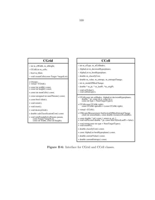
![169
CTask
− static int m_classInstanceCount;
− int m_id;
− int m_actionIndex, m_sensorIndex, m_modeIndex;
− PG * m_policyGraphs;
− int m_nNumActions, m_nCurrentDepth, m_nHorizon;
− int m_nInitNodeIndex;
− int m_strategyIndex;
− double * m_resourcesForTask/*[TotalSensorCount]*/;
− double m_value;
− double m_measureWeight;
− void setResourcesForTask(const bool reinit = false);
− void setTaskValue();
+ CTask(CCell& cell, const int sensorIndex, const int modeIndex);
+ CTask(CCell& cell, PG * policy_graphs, int currentDepth,
int numActions, int horizon, int initNodeIndex, int strategyIndex,
const double * resourcesForTask = NULL);
+ virtual ~CTask();
+ const int actionIndex() const;
+ const int sensorIndex() const;
+ const int modeIndex() const;
+ const int strategyIndex() const;
+ const int id() const;
+ const double value() const;
+ const int initNodeIndex() const;
+ const int numActions() const;
+ const int currentDepth() const;
+ const int horizon() const;
+ double measureWeight() const;
+ double resourcesForTask(const int sensorIndex);
+ double resourcesForTask() const;
+ const double * resourcesForTaskPtr() const;
+ void setMeasureWeight(const double weight);
+ int nextNodeIndex(int obs) const;
+ CTask createFollowUpTask(int obs,
const double * remainingResourceCost/*[TotalSensorCount]*/);
+ void computeRemainingResourceCost(
double * remainingResourceCost/*[TotalSensorCount]*/, int obs) const;
+ bool operator < (const CTask& right) const;
+ CCell& cell() const;
+ static const int classInstanceCount();
+ static void resetClassInstanceCount();
Figure B·7: Interface for CTask class.](https://image.slidesharecdn.com/9f5467db-22a0-4b25-9f85-d66c2d62a6f8-160910233158/85/dissertation-191-320.jpg)