DS

1. DATA STRUCTURES

2. Basic terminologies
 Linear and Nonlinear data structures
 Algorithm: Definition
Pseudo code
Analysis – Design Techniques
INTRODUCTION

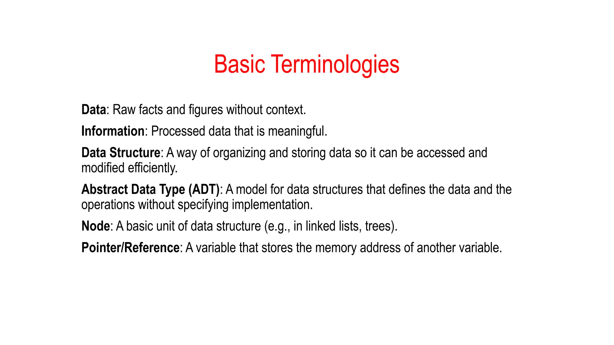
3. Basic Terminologies
Data: Raw facts and figures without context.
Information: Processed data that is meaningful.
Data Structure: A way of organizing and storing data so it can be accessed and
modified efficiently.
Abstract Data Type (ADT): A model for data structures that defines the data and the
operations without specifying implementation.
Node: A basic unit of data structure (e.g., in linked lists, trees).
Pointer/Reference: A variable that stores the memory address of another variable.

4. Linear Data Structures
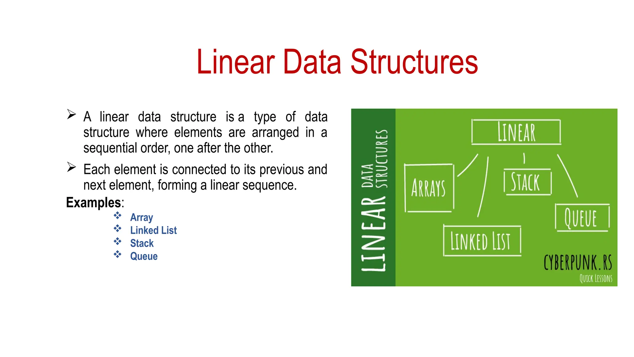
 A linear data structure is a type of data
structure where elements are arranged in a
sequential order, one after the other.
 Each element is connected to its previous and
next element, forming a linear sequence.
Examples:
 Array
 Linked List
 Stack
 Queue

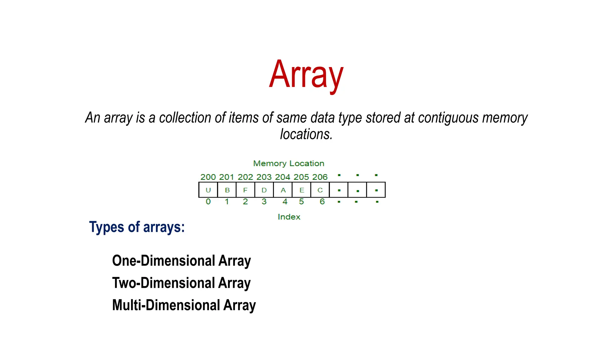
5. Array
An array is a collection of items of same data type stored at contiguous memory
locations.
Types of arrays:
One-Dimensional Array
Two-Dimensional Array
Multi-Dimensional Array

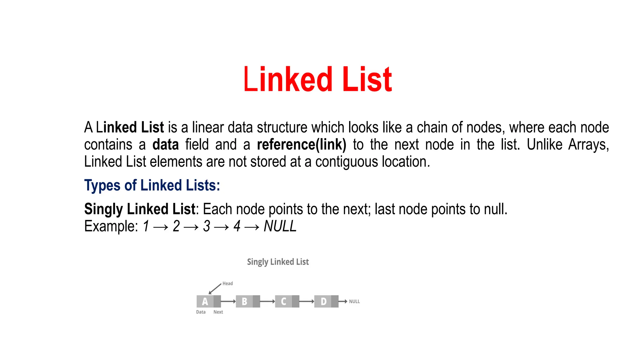
6. Linked List
A Linked List is a linear data structure which looks like a chain of nodes, where each node
contains a data field and a reference(link) to the next node in the list. Unlike Arrays,
Linked List elements are not stored at a contiguous location.
Types of Linked Lists:
Singly Linked List: Each node points to the next; last node points to null.
Example: 1 → 2 → 3 → 4 → NULL

7. Linked List (con)
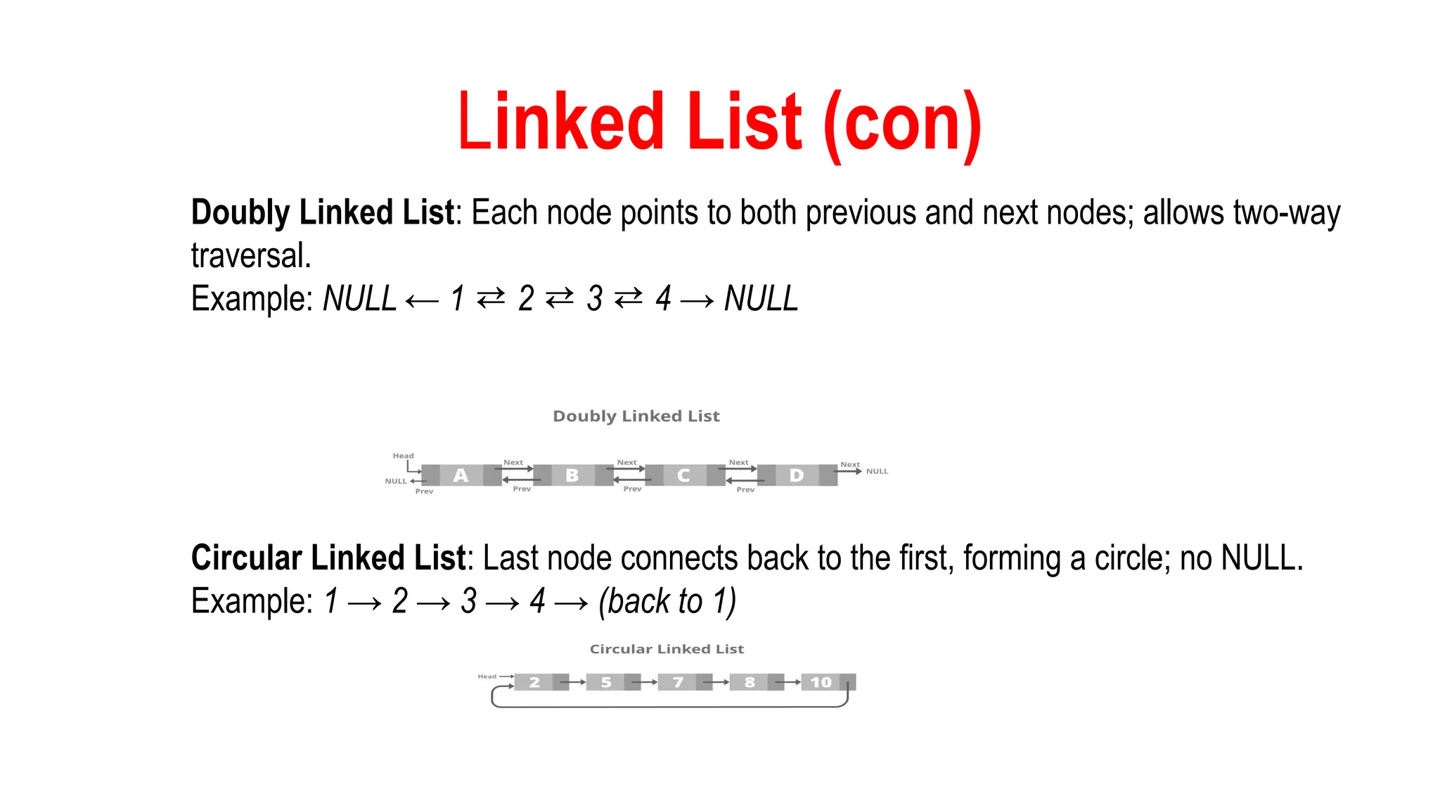
Doubly Linked List: Each node points to both previous and next nodes; allows two-way
traversal.
Example: NULL ← 1 2 3 4 → NULL
⇄ ⇄ ⇄
Circular Linked List: Last node connects back to the first, forming a circle; no NULL.
Example: 1 → 2 → 3 → 4 → (back to 1)

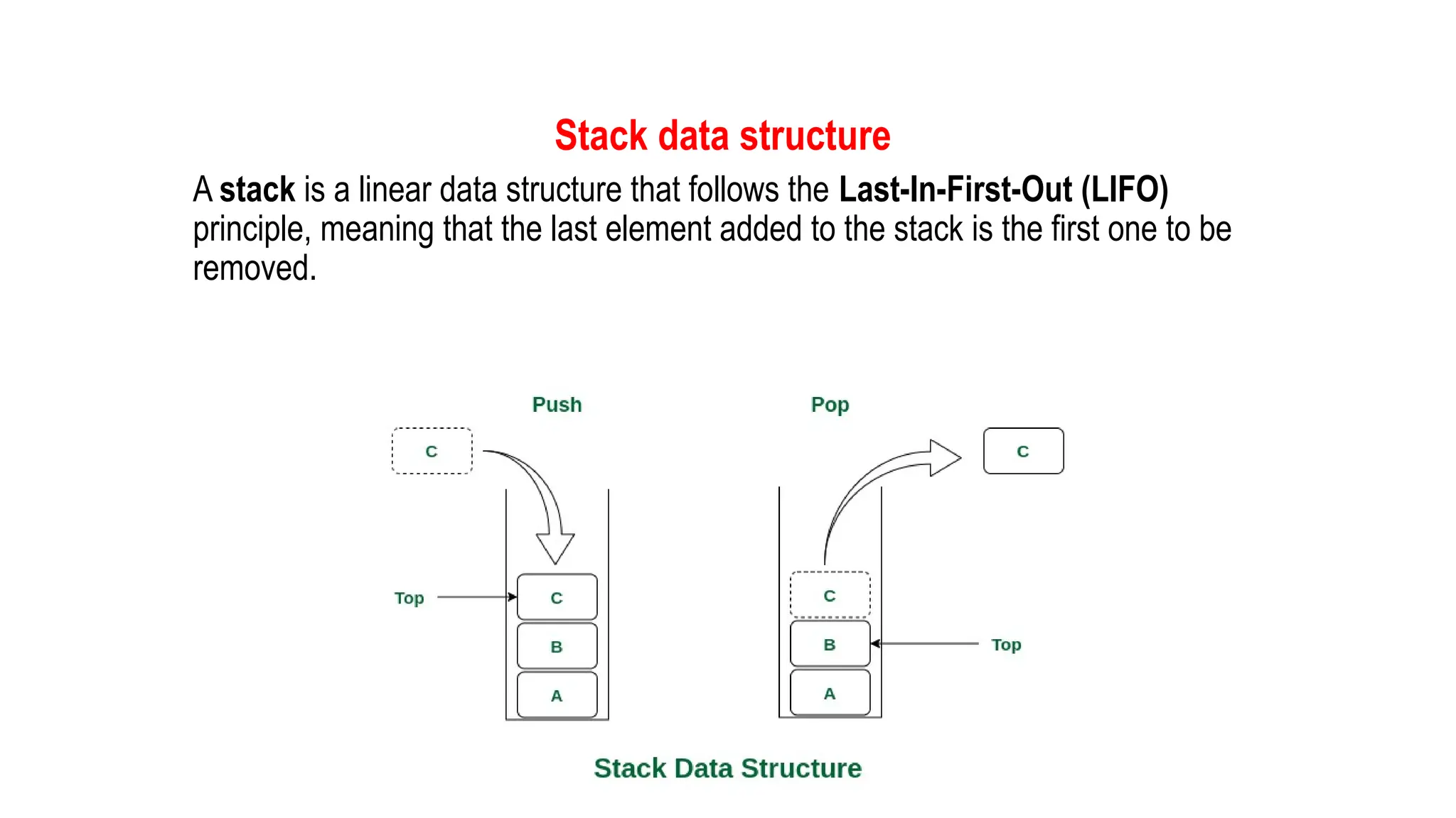
8. Stack data structure
A stack is a linear data structure that follows the Last-In-First-Out (LIFO)
principle, meaning that the last element added to the stack is the first one to be
removed.

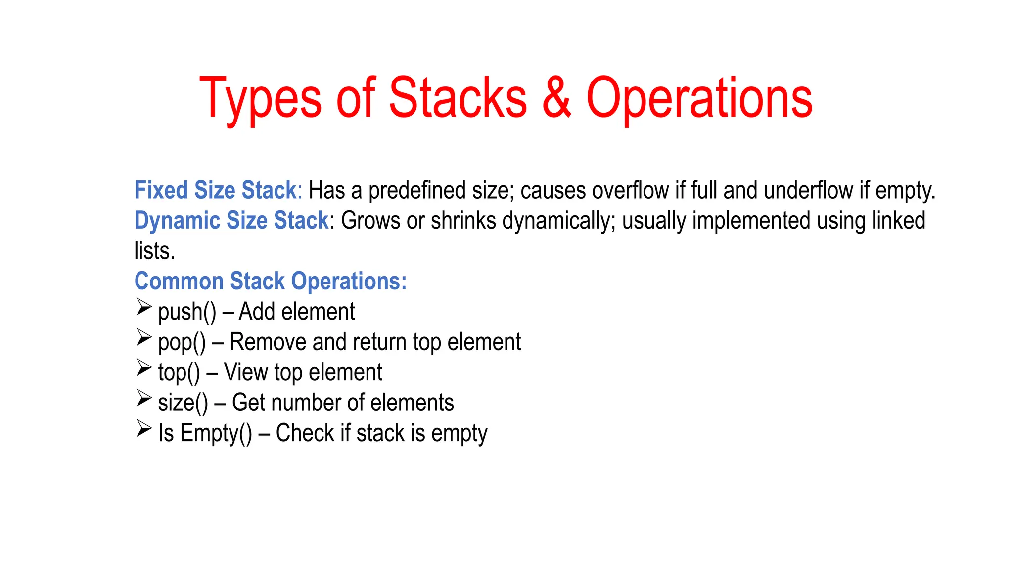
9. Types of Stacks & Operations
Fixed Size Stack: Has a predefined size; causes overflow if full and underflow if empty.
Dynamic Size Stack: Grows or shrinks dynamically; usually implemented using linked
lists.
Common Stack Operations:
push() – Add element
pop() – Remove and return top element
top() – View top element
size() – Get number of elements
Is Empty() – Check if stack is empty

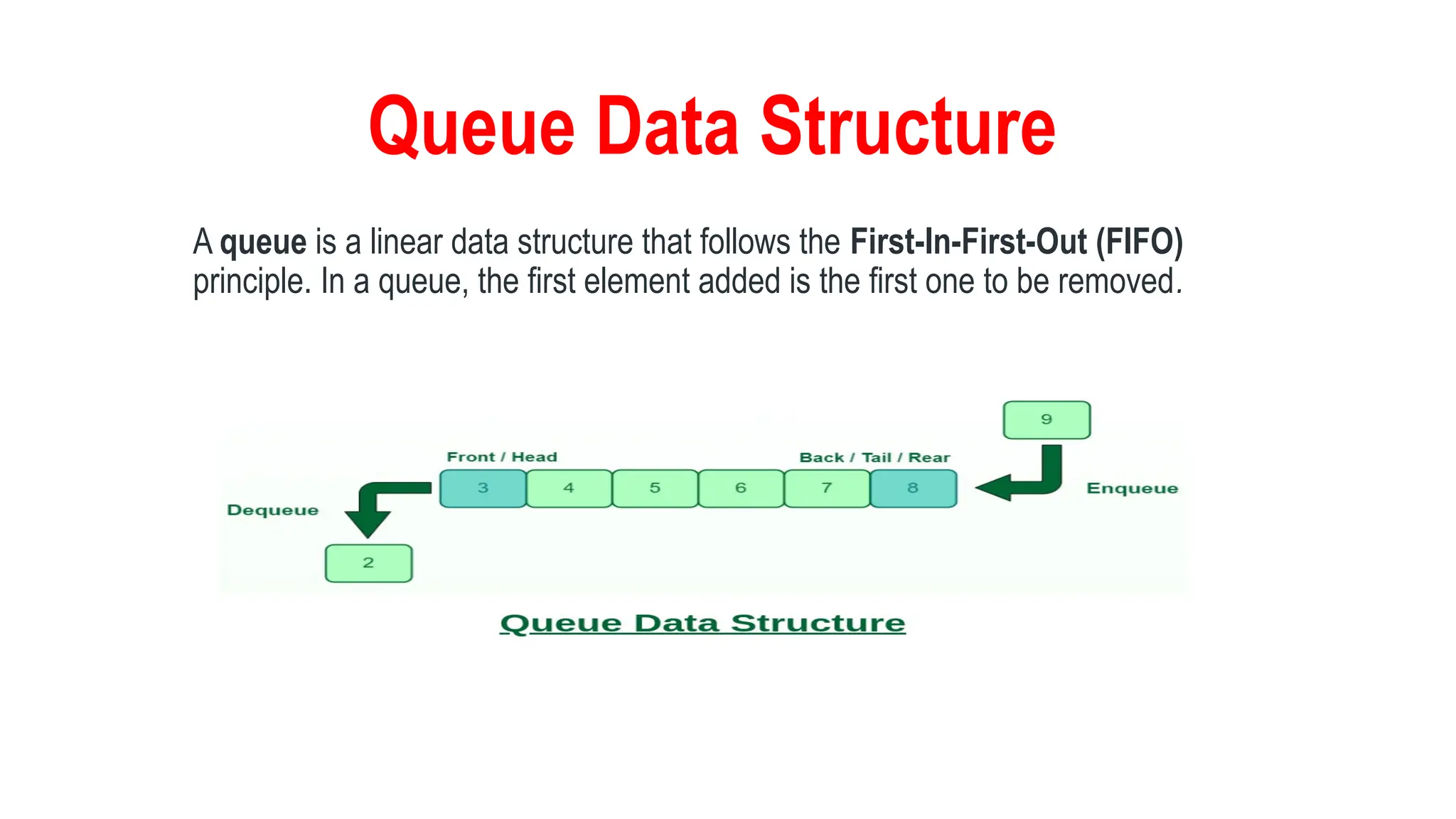
10. Queue Data Structure
A queue is a linear data structure that follows the First-In-First-Out (FIFO)
principle. In a queue, the first element added is the first one to be removed.

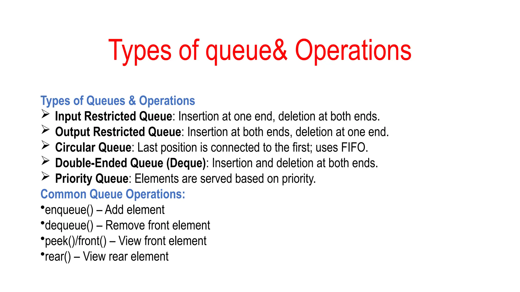
11. Types of queue& Operations
Types of Queues & Operations
 Input Restricted Queue: Insertion at one end, deletion at both ends.
 Output Restricted Queue: Insertion at both ends, deletion at one end.
 Circular Queue: Last position is connected to the first; uses FIFO.
 Double-Ended Queue (Deque): Insertion and deletion at both ends.
 Priority Queue: Elements are served based on priority.
Common Queue Operations:
•enqueue() – Add element
•dequeue() – Remove front element
•peek()/front() – View front element
•rear() – View rear element

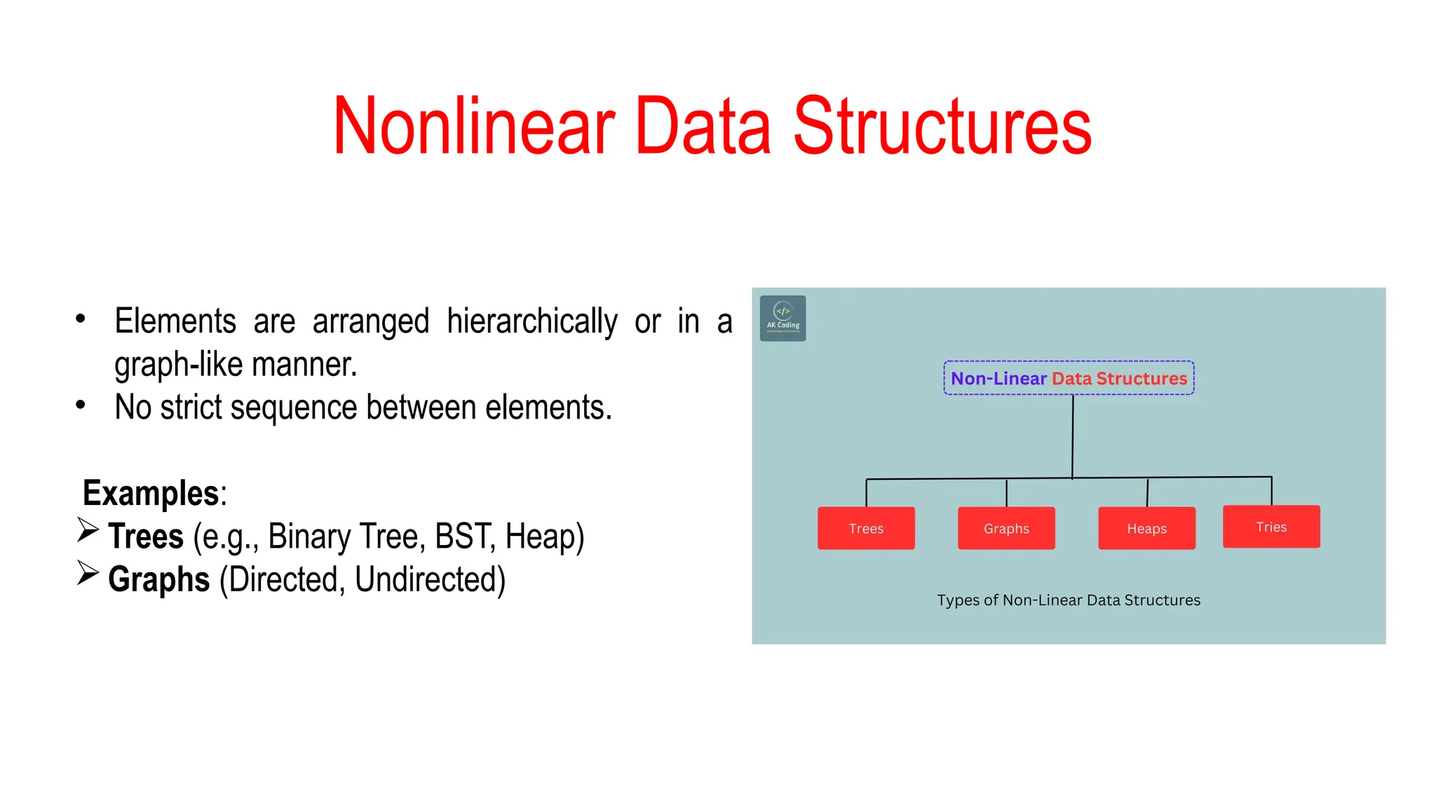
12. Nonlinear Data Structures
• Elements are arranged hierarchically or in a
graph-like manner.
• No strict sequence between elements.
Examples:
Trees (e.g., Binary Tree, BST, Heap)
Graphs (Directed, Undirected)

13. Tree Data Structure
A hierarchical structure with a root and child nodes; used to represent
relationships efficiently.
Types of Trees:
 Simple Tree: One root, multiple children; no cycles.
 Binary Tree: Max two children per node.
 Binary Search Tree (BST): Left < Parent < Right.
 AVL Tree: Self-balancing BST with height difference ≤ 1.
 B-Tree: Multi-child, balanced tree for fast search, insert, delete.

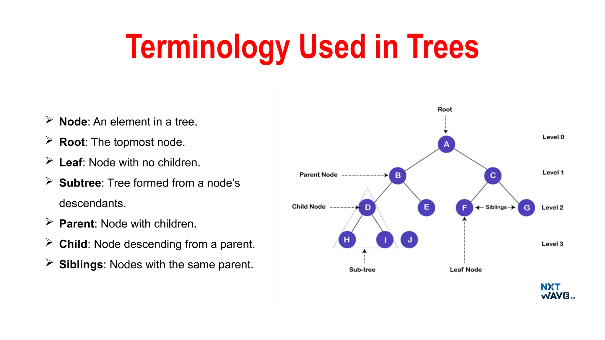
14. Terminology Used in Trees
 Node: An element in a tree.
 Root: The topmost node.
 Leaf: Node with no children.
 Subtree: Tree formed from a node’s
descendants.
 Parent: Node with children.
 Child: Node descending from a parent.
 Siblings: Nodes with the same parent.

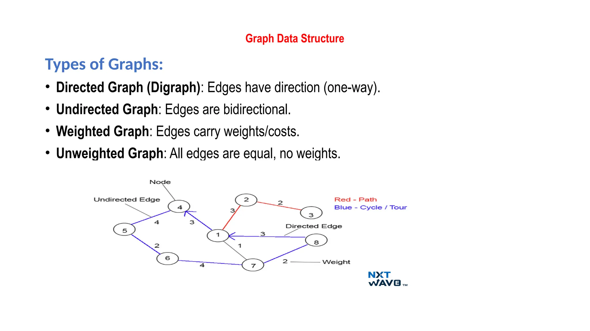
15. Graph Data Structure
Types of Graphs:
• Directed Graph (Digraph): Edges have direction (one-way).
• Undirected Graph: Edges are bidirectional.
• Weighted Graph: Edges carry weights/costs.
• Unweighted Graph: All edges are equal, no weights.

16. Algorithm
An algorithm is a step-by-step set of instructions to solve a problem or perform a task.
It is fundamental to computer science and crucial for designing efficient solutions in data
structures and programming.
Example:
Algorithm: Find the Largest Number in an Array
Problem:
Given an array of n numbers, find the largest number.
Algorithm Steps:
1.
Start
2.
Initialize max = arr[0]
3.
For each element arr[i] in the array (from index 1 to n-1):
a. If arr[i] > max, then max = arr[i]
4.
End loop
5.
Return max
6.
Stop

17. Start
Initialize max ← arr[0]
For i ← 1 to n - 1 do
If arr[i] > max then
max ← arr[i]
End If
End For
Return max
Stop
Pseudocode for finding the maximum element in an array:

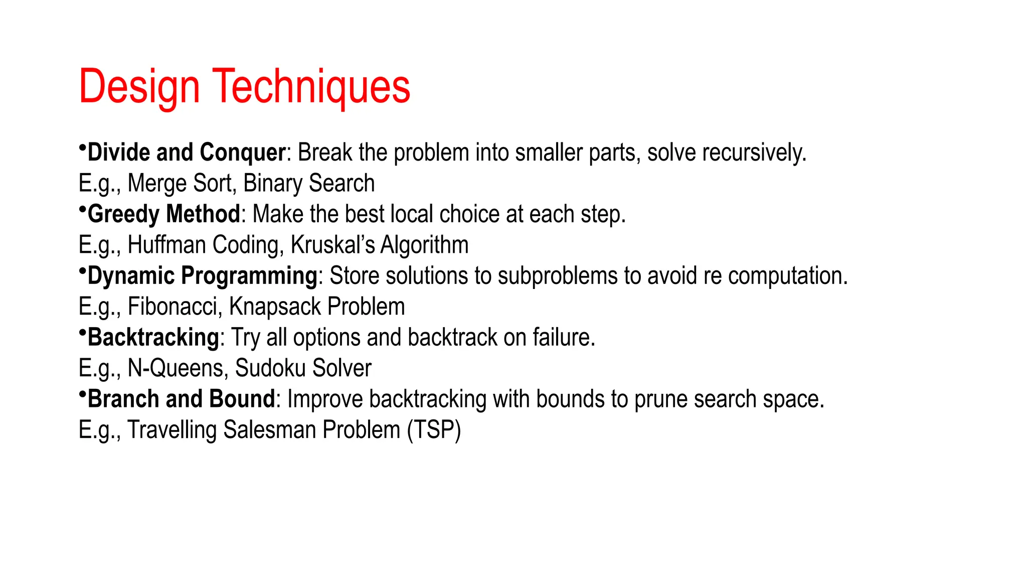
18. Design Techniques
•Divide and Conquer: Break the problem into smaller parts, solve recursively.
E.g., Merge Sort, Binary Search
•Greedy Method: Make the best local choice at each step.
E.g., Huffman Coding, Kruskal’s Algorithm
•Dynamic Programming: Store solutions to subproblems to avoid re computation.
E.g., Fibonacci, Knapsack Problem
•Backtracking: Try all options and backtrack on failure.
E.g., N-Queens, Sudoku Solver
•Branch and Bound: Improve backtracking with bounds to prune search space.
E.g., Travelling Salesman Problem (TSP)

19. THANK YOU