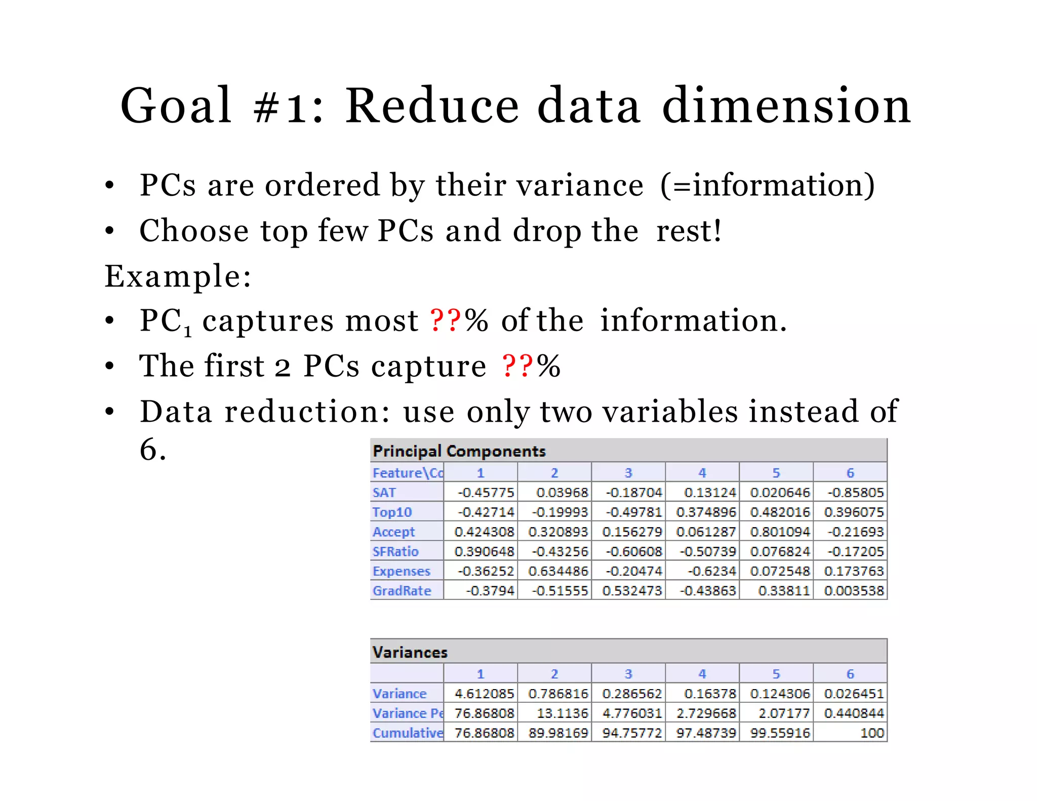
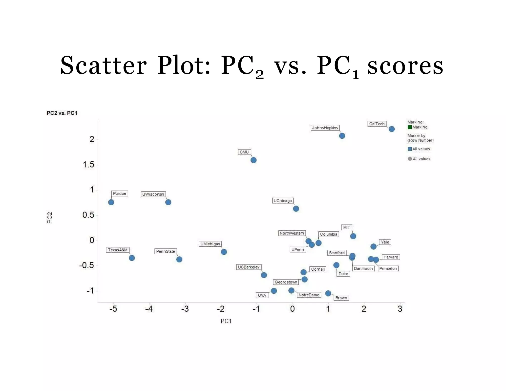
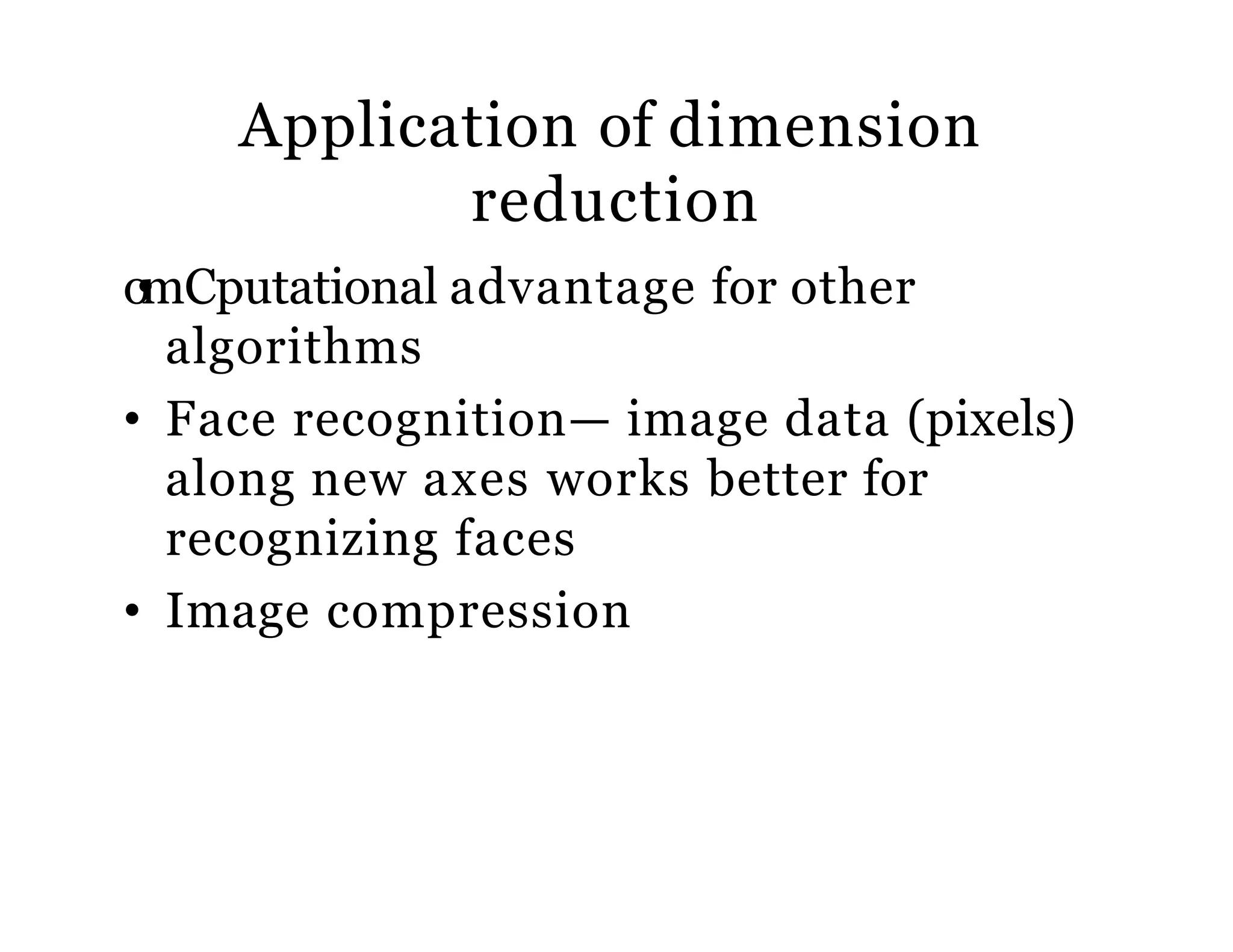
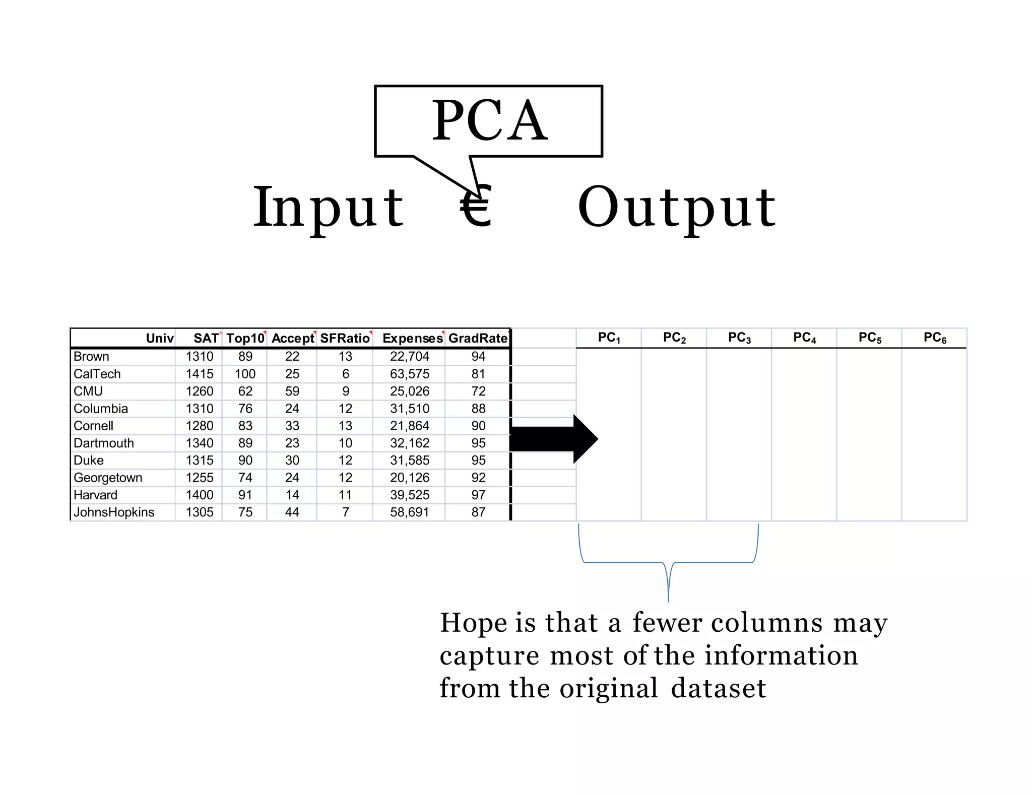
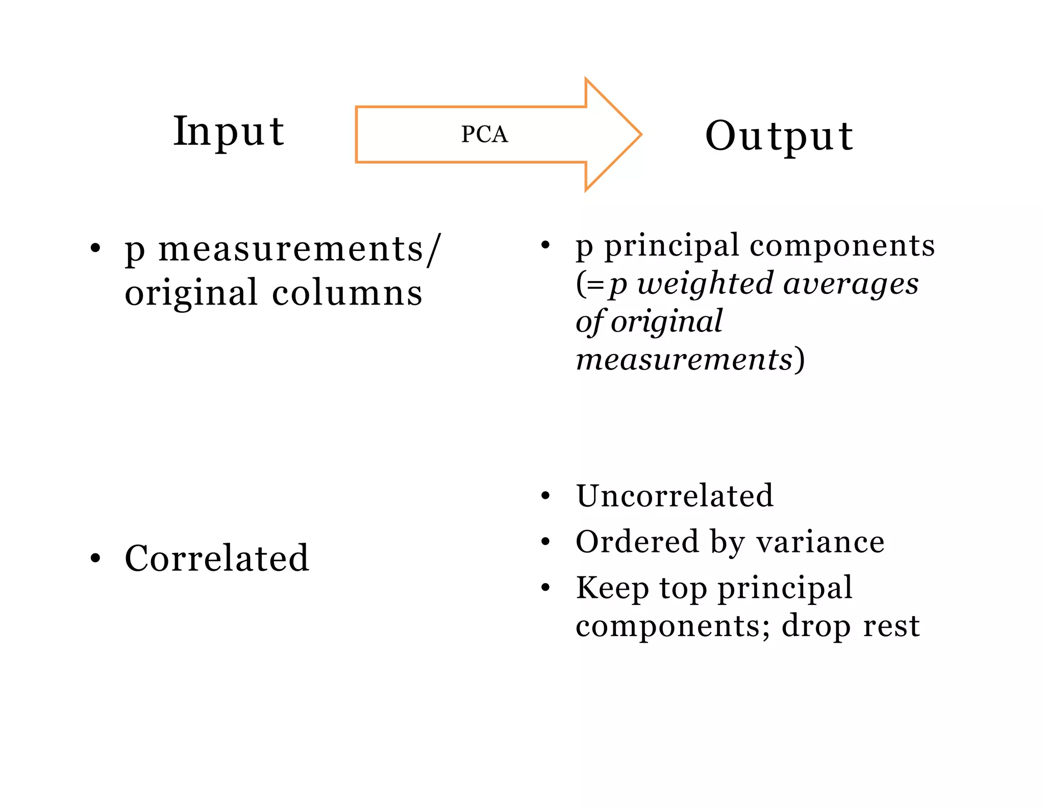
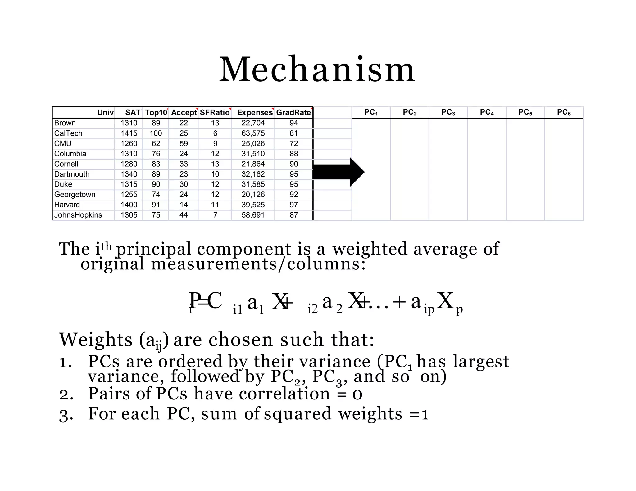
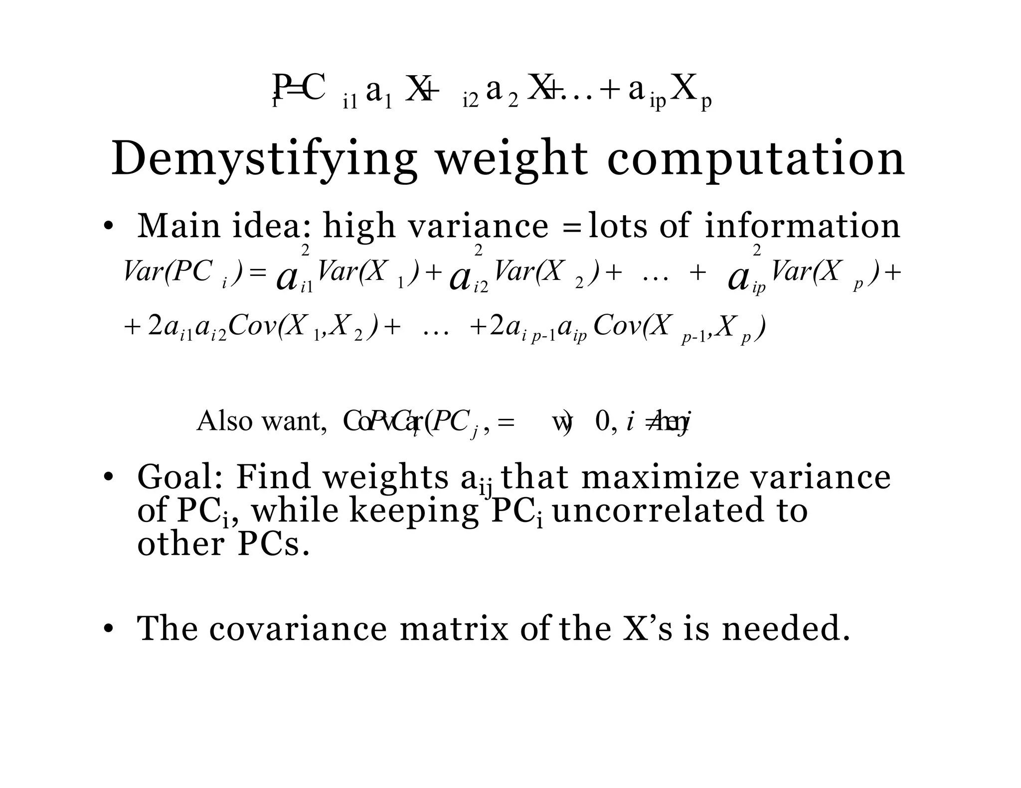
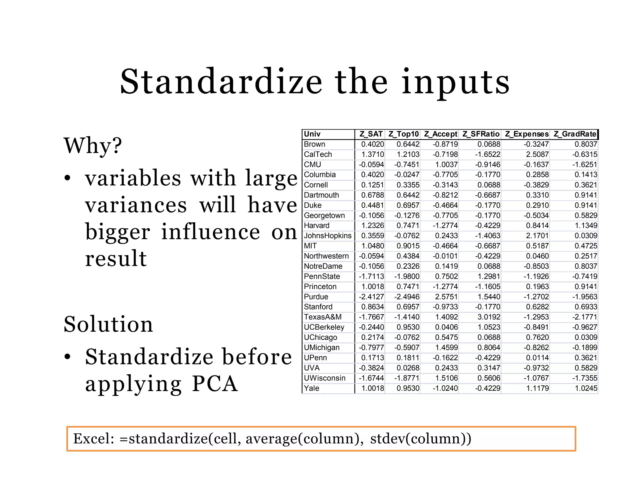
ExcelR is a global leader delivering a wide gamut of management and technical training over 40 countries. We are a trusted training delivery partner of 350+ corporate clients and universities across the globe with 140,000+ professionals trained across various courses.
5. Input € Output
Univ SAT Top10 Accept SFRatio Expenses GradRate PC1 PC2 PC3 PC4 PC5 PC6
Brown 1310 89 22 13 22,704 94
CalTech 1415 100 25 6 63,575 81
CMU 1260 62 59 9 25,026 72
Columbia 1310 76 24 12 31,510 88
Cornell 1280 83 33 13 21,864 90
Dartmouth 1340 89 23 10 32,162 95
Duke 1315 90 30 12 31,585 95
Georgetown 1255 74 24 12 20,126 92
Harvard 1400 91 14 11 39,525 97
JohnsHopkins 1305 75 44 7 58,691 87
Hope is that a fewer columns may
capture most of the information
from the original dataset
PCA
6. The Primitive Idea –Intuition
First
How to compress the data
loosing the least amount of information?
7. Input
• p measurements/
original columns
• Correlated
Output
• p principal components
(=p weighted averages
of original
measurements)
• Uncorrelated
• Ordered by variance
• Keep top principal
components; drop rest
PCA
8. Mechanism
The ith principal component is a weighted average of
original measurements/columns:
Weights (aij) are chosen such that:
1. PCs are ordered by their variance (PC1 has largest
variance, followed by PC2, PC3, and so on)
2. Pairs of PCs have correlation = 0
3. For each PC, sum of squared weights =1
i1 a1 XiPC i2 a2 X aip Xp
Univ SAT Top10 Accept SFRatio Expenses GradRate PC1 PC2 PC3 PC4 PC5 PC6
Brown 1310 89 22 13 22,704 94
CalTech 1415 100 25 6 63,575 81
CMU 1260 62 59 9 25,026 72
Columbia 1310 76 24 12 31,510 88
Cornell 1280 83 33 13 21,864 90
Dartmouth 1340 89 23 10 32,162 95
Duke 1315 90 30 12 31,585 95
Georgetown 1255 74 24 12 20,126 92
Harvard 1400 91 14 11 39,525 97
JohnsHopkins 1305 75 44 7 58,691 87
9. Demystifying weight computation
• Main idea: high variance = lots of information
pipi a a aVar(PC )
Also want, CoPvCair(PCj , w) 0, i henj
• Goal: Find weights aij that maximize variance
of PCi, while keeping PCi uncorrelated to
other PCs.
• The covariance matrix of the X’s is needed.
p-1,X p ) 2ai p-1aip Cov(X 2ai1ai2Cov(X 1,X 2 )
2
Var(X )1 2
2 2
Var(X ) Var(X ) i1 i2
i1 a1 XiPC i2 a2 X aip Xp
11. Standardization shortcut for PCA
• Rather than standardize the data
manually, you can use correlation
matrix instead of covariance matrix
as input
• PCA with and without standardization
gives different results!
12. PCA
Transform > Principal Components
(correlation matrix has been used here)
• PCs are uncorrelated
• Var(PC1) > Var (PC2)
> ...
PCi ai1X1 ai2X2 aip Xp
Scaled Data PC Scores
Principal
Components
13. Computing principal scores
• For each record, we can compute their score
on each PC.
• Multiply each weight (aij) by the appropriate
Xij
• Example for Brown University (using
standardized numbers):
• PC Score1 for Brown University = (–
0.458)(0.40) +(–0.427)(.64) +(0.424)(–0.87)
+(0.391)(.07) + (–0.363)(–0.32) + (–0.379)(.80) =
–0.989
14. R Code for PCA (Assignment)
OPTIONAL RCode
install.packages("gdata") ##for reading xls files
install.packages("xlsx") ## ”for reading xlsxfiles
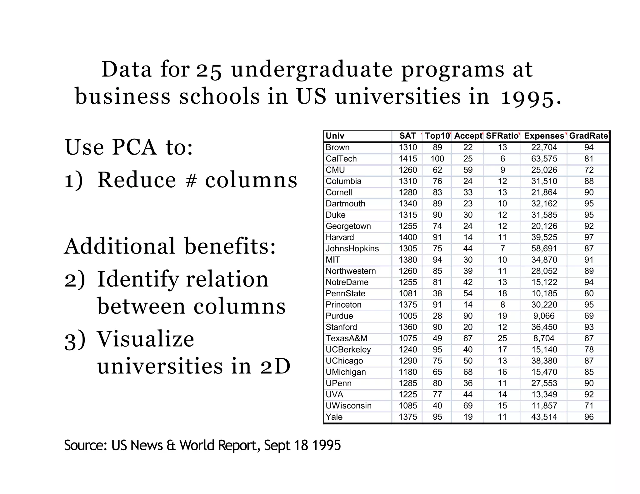
mydata<-read.xlsx("UniversityRanking.xlsx",1) ## use read.csv for csv files
mydata## make sure the datais loadedcorrectly
help(princomp) ## to understand the api for princomp
pcaObj<-princomp(mydata[1:25,2:7], cor = TRUE, scores = TRUE, covmat = NULL)
## the first column in mydatahas universitynames
## princomp(mydata,cor = TRUE) not_same_as prcomp(mydata,scale=TRUE);similar,but different
summary(pcaObj)
loadings(pcaObj)
plot(pcaObj)
biplot(pcaObj)
pcaObj$loadings
pcaObj$scores
15. Goal #1: Reduce data dimension
• PCs are ordered by their variance (=information)
• Choose top few PCs and drop the rest!
Example:
• PC1 captures most ??% of the information.
• The first 2 PCs capture ??%
• Data reduction: use only two variables instead of
6.
16. Matrix Transpose
OPTIONAL: R code
help(matrix)
A<-matrix(c(1,2),nrow=1,ncol=2,byrow=TRUE)
A
t(A)
B<-matrix(c(1,2,3,4),nrow=2,ncol=2,byrow=TRUE)
B
t(B)
C<matrix(c(1,2,3,4,5,6),nrow=3,ncol=2,byrow=TRUE)
C
t(C)
20. Goal #2: Learn relationships with
PCA by interpreting the weights
• ai1,…, aip are the coefficients for PCi.
• They describe the role of original X
variables in computing PCi.
• Useful in providing context-specific
interpretation of each PC.
21. PC1 Scores
(choose one or more)
1. are approximately a simple average of
the 6 variables
2. measure the degree of high Accept &
SFRatio, but low Expenses, GradRate,
SAT, and Top10
22. Goal #3: Use PCA for visualization
•heTfirst 2 (or 3) PCs provide a way to
project the data from a p-dimensional
space onto a 2D (or 3D) space
24. Monitoring batch processes
using PCA
u•lMtivariatedata at different time points
• Historical database of successful batches
are used
• Multivariate trajectory data is projected
to low-dimensional space
>>> Simple monitoring charts to spot outlier
25. Your Turn!
1. If we use a subset of the principal
components, is this useful for
prediction? for explanation?
2. What are advantages and
weaknesses of PCA compared to
choosing a subset of the variables?
3. PCA vs. Clustering