The document outlines several algorithms including binary search, merge sort, quick sort, and selection sort along with their time complexities and theoretical steps for implementation. It also discusses Prim's and Kruskal's algorithms for finding minimum spanning trees, as well as the functionality, applications, and challenges of parallel algorithms. Each section provides fundamental differences in the algorithms, practical implementation considerations, and examples to illustrate their use.

1. 1. Write an algorithms for:
 Binary search
 Merge sort
 Quick sort
 Selection sort
 Binary Search: A search algorithm that efficiently finds a target value in a sorted array.
 Merge Sort: A divide-and-conquer algorithm that recursively divides an array into smaller
subarrays, sorts them, and merges them back together.
 Quick Sort: Another divide-and-conquer algorithm that partitions an array around a pivot
element and recursively sorts the partitions.
 Selection Sort: A simple algorithm that repeatedly finds the minimum element in the
unsorted portion of the array and swaps it with the first unsorted element.
Theoretical Steps for Each Algorithm
 Binary Search:
1. Initialize pointers: Set left to 0 and right to the array's length - 1.
2. Check for empty array: If left is greater than right, return -1 (not found).
3. Calculate the middle index: mid = (left + right) / 2.
4. Compare:
 If target is equal to arr[mid], return mid.
 If target is less than arr[mid], update right to mid - 1.
 If target is greater than arr[mid], update left to mid + 1.
5. Repeat steps 2-4 until the target is found or the search space is exhausted.
 Merge Sort:
1. Divide: If the array's length is greater than 1, divide it into two halves.
2. Conquer: Recursively sort the left and right halves.
3. Combine: Merge the sorted halves into a single sorted array.
 Quick Sort:
1. Partition: Choose a pivot element (e.g., the last element) and partition the array into two
subarrays: one with elements less than the pivot and one with elements greater than or
equal to the pivot.
2. Recursively sort: Recursively sort the left and right subarrays.
 Selection Sort
1. Iterate through the array: For each element from the beginning to the second-to-last
element:
 Find the minimum: Find the index of the minimum element in the unsorted portion
of the array.
 Swap: Swap the current element with the minimum element.
Note on Practical Implementation
While the theoretical steps provide a solid foundation, practical implementations often involve additional
considerations, such as:
 Data structures: Choosing appropriate data structures (e.g., arrays, linked lists) for the
specific use case.
ODAA BULTUM UNIVERSITY
COLLEGE OF NATURAL SCIENCE
AND COMPUTATIONAL SCIENCE
DEPARTMENT OF COMPUTER SCIENCE
Design and analysis of algorithm course. Submitted date:
Individual. September 12/2024
Name Id.No
1. Shafi Esa ——————— 1919 Submitted to:
MSc. HADI . H

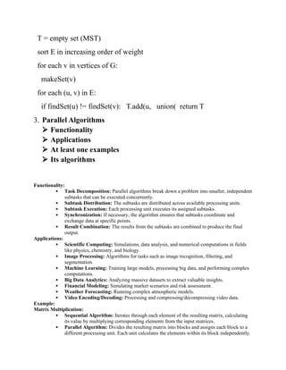
2.  Edge cases: Handling special cases like empty arrays, arrays with duplicates, or arrays
with very large or small elements.
 Performance optimization: Employing techniques like tail-call optimization or in-place
partitioning to improve efficiency.

1. Write the time complexity for the following algorithms by taking
at least one examples
 Binary search
 Merge sort
 Quick sort
 Selection sort
 Binary Search:
 Time complexity: O(log n)
 Example:
 Input: Sorted array of integers [1, 2, 3, 4, 5, 6, 7, 8, 9]
 Target: 5
 Algorithm:
1. Start with the middle element (5).
2. Since 5 is equal to the target, return the index (4).
 Merge Sort:
 Time complexity: O(n log n)
 Example:
 Input: Unsorted array of integers [3, 2, 5, 1, 4]
 Algorithm:
1. Divide the array into two halves: [3, 2] and [5, 1, 4].
2. Recursively sort each half: [2, 3] and [1, 4, 5].
3. Merge the sorted halves: [1, 2, 3, 4, 5].
 Quick Sort:
 Time complexity: O(n^2) in the worst case, O(n log n) on
average
 Example:
 Input: Unsorted array of integers [5, 3, 8, 2, 1]

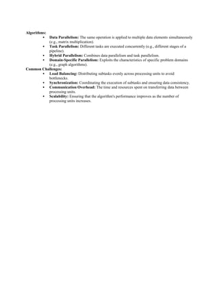
3.  Algorithm:
1. Choose a pivot (e.g., 5).
2. Partition the array around the pivot: [2, 1, 3, 5, 8].
3. Recursively sort the left and right subarrays.
 Selection Sort:
 Time complexity: O(n^2)
 Example:
 Input: Unsorted array of integers [3, 2, 5, 1, 4]
 Algorithm:
1. Find the minimum element (1) and swap it with the
first element.
2. Find the minimum element in the remaining unsorted
part (2) and swap it with the second element.
3. Repeat until the entire array is sorted
2. Write an algorithm for:
 Prims algorithm
 Kruskal’s algorithm
Prim's Algorithm
Purpose: To find the minimum spanning tree (MST) of a weighted
undirected graph.
 Algorithm:
1.Initialization:
 Choose any vertex as the starting vertex.
 Create an empty set to store the edges of the MST.
 Create a set to store vertices that are part of the MST.
2. Iteration:

4.  While the set of vertices in the MST is not equal to the total
number of vertices:
 Find the edge with the minimum weight that connects a
vertex in the MST to a vertex not in the MST.
 Add this edge to the MST and the corresponding vertex to
the set of vertices in the MST.
3. Return:
 Return the MST.
Pseudo code:
Prim's Algorithm(G):
V = vertices of G
E = edges of G
T = empty set (MST)
Q = min-heap of vertices
for each v in V:
key[v] = infinity
prev[v] = null
choose any vertex u as the starting vertex
key[u] = 0
Q.insert(u)
while Q is not empty:
u = Q.extractMin()
for each v in adj[u]:

5. if v is in Q and weight(u, v) < key[v]:
prev[v] = u
key[v] = weight(u, v)
Q.decreaseKey(v, key[v]) construct MST T using prev array
returnT
 Kruskal's Algorithm
Purpose: To find the minimum spanning tree (MST) of a weighted
undirected graph.
 Algorithm:
1.Initialization:
 Sort the edges in increasing order of their weights.
 Create an empty set to store the edges of the MST.
 Create a disjoint set data structure to represent the connected
components of the graph.
2. Iteration:
 For each edge in the sorted list:
 If the edges do not form a cycle, add it to the MST and union
the corresponding sets in the disjoint set data structure.
3.Return:
 Return the MST.
Pseudo code:
Kruskal's Algorithm(G):
E = edges of G

6. T = empty set (MST)
sort E in increasing order of weight
for each v in vertices of G:
makeSet(v)
for each (u, v) in E:
if findSet(u) != findSet(v): T.add(u, union( return T
3. Parallel Algorithms
 Functionality
 Applications
 At least one examples
 Its algorithms
Functionality:
 Task Decomposition: Parallel algorithms break down a problem into smaller, independent
subtasks that can be executed concurrently.
 Subtask Distribution: The subtasks are distributed across available processing units.
 Subtask Execution: Each processing unit executes its assigned subtasks.
 Synchronization: If necessary, the algorithm ensures that subtasks coordinate and
exchange data at specific points.
 Result Combination: The results from the subtasks are combined to produce the final
output.
Applications:
 Scientific Computing: Simulations, data analysis, and numerical computations in fields
like physics, chemistry, and biology.
 Image Processing: Algorithms for tasks such as image recognition, filtering, and
segmentation.
 Machine Learning: Training large models, processing big data, and performing complex
computations.
 Big Data Analytics: Analyzing massive datasets to extract valuable insights.
 Financial Modeling: Simulating market scenarios and risk assessment.
 Weather Forecasting: Running complex atmospheric models.
 Video Encoding/Decoding: Processing and compressing/decompressing video data.
Example:
Matrix Multiplication:
 Sequential Algorithm: Iterates through each element of the resulting matrix, calculating
its value by multiplying corresponding elements from the input matrices.
 Parallel Algorithm: Divides the resulting matrix into blocks and assigns each block to a
different processing unit. Each unit calculates the elements within its block independently.

7. Algorithms:
 Data Parallelism: The same operation is applied to multiple data elements simultaneously
(e.g., matrix multiplication).
 Task Parallelism: Different tasks are executed concurrently (e.g., different stages of a
pipeline).
 Hybrid Parallelism: Combines data parallelism and task parallelism.
 Domain-Specific Parallelism: Exploits the characteristics of specific problem domains
(e.g., graph algorithms).
Common Challenges:
 Load Balancing: Distributing subtasks evenly across processing units to avoid
bottlenecks.
 Synchronization: Coordinating the execution of subtasks and ensuring data consistency.
 Communication Overhead: The time and resources spent on transferring data between
processing units.
 Scalability: Ensuring that the algorithm's performance improves as the number of
processing units increases.