This document outlines a vulnerability project analyzing flood and social vulnerability in Maryland. Data on population, housing, and demographics from 2006-2010 will be used to create vulnerability indices from 0-1 at the census block group level. Flood vulnerability will be calculated based on elevation thresholds from 0-1 meters, and social vulnerability will be the average of normalized socioeconomic indicators. The two raster maps will be combined through multiplication to create a final vulnerability map. An analysis found some block groups had higher vulnerability indices than others due to social factors. Limitations include data processing errors and other social variables that could provide more context. Further analysis estimated over 35,000 people were in the areas of very high combined vulnerability.

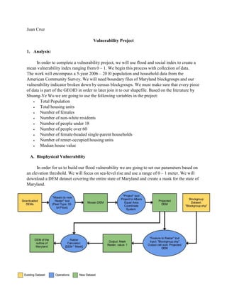
1. Juan Cruz
Vulnerability Project
1. Analysis:
In order to complete a vulnerability project, we will use flood and social index to create a
mean vulnerability index ranging from 0 – 1. We begin this process with collection of data.
The work will encompass a 5-year 2006 – 2010 population and household data from the
American Community Survey. We will need boundary files of Maryland blockgroups and our
vulnerability indicator broken down by census blockgroups. We must make sure that every piece
of data is part of the GEOID in order to later join it to our shapefile. Based on the literature by
Shuang-Ye Wu we are going to use the following variables in the project:
 Total Population
 Total housing units
 Number of females
 Number of non-white residents
 Number of people under 18
 Number of people over 60
 Number of female-headed single-parent households
 Number of renter-occupied housing units
 Median house value
A. Biophysical Vulnerability
In order for us to build our flood vulnerability we are going to set our parameters based on
an elevation threshold. We will focus on sea-level rise and use a range of 0 – 1 meter. We will
download a DEM dataset covering the entire state of Maryland and create a mask for the state of
Maryland.

2. In order to calculate our index for sea-level rise we will use a 0 – 1 meter range, this range
is built as follows:
0: Elevation > 1 meters; Elevation < 0 meters
1: Elevation .8-1 meters
2: Elevation .6-.8 meters
3: Elevation .4-.6 meters
4: Elevation .2-.4 meters
5: Elevation 0-.2 meters
To set up this range we reclassify the DEM mask of Maryland previously created:
The raster dataset indicates
our vulnerability index for
flooding and what is the
location of the hazardous areas.
The blockgroups having areas
of elevation between 0 - .2
meters are at most risk of
flooding. This variable will be
combined with social variables
to see which blockgroups are
more vulnerable to hazard.

3. B. Social Vulnerability
To calculate social vulnerability we must create a vulnerability index ranging from 0 – 1 of
all of our social variables and then come up with a mean vulnerability index for every
blockgroup. The computation based on Susan L. Cutter literature outlines the steps to create a
vulnerability index, this is easily done in Excel:
1. Find the ratio of the variable in each blockgroup to the total number of that variable in the
state.
Ratio Variable =
Blockgroup Variable
State Total of that Variable
2. Divide the particular ratio (X) by the maximum value (maxX) to create an index between
0 to 1. Repeat up to step 2 for all variables except “median house value”. In this case, we
must eliminate any negative ratio quantities by absolute value.
Vulnerability =
Absolute (Ratio (X))
Maximum (maxX)
3. Take the average of all vulnerability numbers in each blockgroup to create a final
vulnerability index for that blockgroup.
Final Vulnerability Index =
∑(Vulnerability number of every social variable)
Number of Variables (n)
Now that have the final social vulnerability, we export this tabular data as a DBF file. Then
we make a relational join based on the GEOID of the blockgroups. Lastly, we must make this
relational dataset a raster to combine it with the biophysical vulnerability. The process is
explained as follows:
We then are able to map out this raster data looking at the final social vulnerability of the
state of Maryland. The map is shown below:

4. C. Final Vulnerability
The final step is to combine the social and biophysical vulnerability values. Since both
of these layers are raster files, we are going to the use the “Raster Calculator” tool. We are
going to multiply the values of both rasters in order to combine them. The equation in the
raster calculator is as follows:
Vuln_Final = [biophys_vuln] * [social_vuln]
After using 5 quantile to represent the final vulnerability on a map, the map looks as
follows:

6. 2. Results
As we can see the Final Vulnerability shows only the pixels where we had both biophysical
and social data. Even though we had social vulnerability for all the blockgroups, our flood
threshold of 1 meter was the cut out for the analysis. Anything outside our range had a value of
“0” which became “0” when multiplied with the social index. Our result is the vulnerability of
social and biophysical vulnerability only inside our range of elevation.
For example, by looking at our flood map, we see that “Block Group 2, Census Tract 9709,
Dorchester County, Maryland” and “Block Group 1, Census Tract 9709, Dorchester County,
Maryland” both are located greatly inside our focus elevation range. Since elevation is
continuous and does not follow blockgroup patterns, two similar adjacent blockgroups can have
different vulnerability based on their social variables. The example below illustrates this case.

7. In the analysis we have been able to use our social variables to establish which
blockgroups would receive first response in case of a disaster, allocation of resources and natural
disaster preparedness by the local authorities. After calculating all the social variables we see
that the blockgroup of moderate vulnerability has a vulnerability index of 0.16 and the higher
blockgroup values at 0.25. In the whole state of Maryland, the maximum social vulnerability
index is 0.569.
3. Limitations & Margin of Error
The limitations of the analysis come mainly from the calculations and data prep done in
Excel. For example, the documentation of the ACS data indicated to use sequence 9 for total
population and total housing units. However, upon examining the data closely, the numbers were
representing sample data and not actual totals. Another case of this was when extracting the
“total population under 18 years old” variable. Since the data did not present itself this way, it
was necessary to add all the age groups under 18. There is always a risk for error with extra
manipulation of the original data.
Certain tasks such as sorting sequence numbers and table number lookup require great
attention to detail in order to link the correct information. Any mistake in this part of the data
processing can create errors with the GeoIDs of the data (which we use later to link the data to
the boundary file).
One of the social variables in question was the difference between housing unit and
household. For the analysis we only acquired the total of housing units. If we take in
consideration abandoned or on sale houses, there are questions on how the total number of
housing units alone provide a case for vulnerability or imply aspects about the population. It
would be important to also include total number of households, as it accounts for units of people
living in that blockgroup, especially if more than one household lives inside the housing unit.
Having total number of households will also make sense because it can be compared to the
number of “Female Single Parent Households” variable that we used in the analysis.
There are other variables in this analysis that could’ve provided interesting results.
Variables such as: total homeless population, total number of public schools, transportation
conditions (car ownership, etc.), and proximity to firehouses, police stations, or maintenance
facilities. Also, there are risks for watershed flooding, which may be above the 1 meter range. A
historic data of flooding in the past 20 years could extend the analysis to look at other potential
flooding risks.

8. 4. Further Analysis
Upon concluding this project we can ask following questions of our final vulnerability
index. For example: how many people were in the most vulnerable group? In this portion we will
answer this question and show how we can draw other information from the results of this
project.
In order to find the population number in the “Very High” vulnerability, we have to isolate
this class and calculate the total population at high risk based on the area (sqm) of vulnerability
in each blockgroup. The process is as such:
1. We are going to use the “Reclassify” tool to give it a value of 1 to the “Very High”
category, the other ones can have “No Data”.
2. At this point it is necessary to convert the raster layer into a polygon since we want to
create a spatial analysis with the blockgroup dataset. We use the “Raster into Polygon”
tool.
3. Then we calculate the area of both the blockgroups and the very high vulnerability area
“Most_Vul.shp”.
4. We use the “intersect” tool to combine both data. This way we are bringing the
population data from blockgroups into the vulnerability area, which has the area
calculated.
5. Since we have to combine the vulnerable areas in its corresponding blockgroup. We
“summarize” the tabular data using the GEOID as the base for the summary. This means
there will be only one GEOID and it will add total area of vulnerability inside each
blockgroup. We should end up with a vulnerability area (sqm) per each blockgroup.
6. Then we divide the vulnerability area by the blockgroup area to obtain a ratio. The area
ratio will be used to estimate the number of total population inside the “very high” group.
The equation for the Total Pop. inside a Vulnerability Area (Y) is as follows:
Y =
Vulnerability area (sqm)
Blockgroup area (sqm)
∗ Blockgroup total population
Results:
Profile of “Very High” Vulnerability area:
Number of Blockgroups affected 526
Total Blockgroup population 795,243
Total Blockgroup Area 11,042,068.17 sqkm.
Total Vuln. Area population 35,536
Total Vuln. Area 368,819.68 sqkm.
Average Ratio 0.036