CHAPTER 3
Flexible Budgets,Variances and Management Control
The use of Variances
Variances represent the difference between the cost that was incurred and the budgeted cost.
Each variance wecompute is the difference between an actual result and a budgeted amount. The
budgeted amount is a benchmark, a point of reference from which comparisons may be made.
Variances assist managers in their planning and control decisions. Management byexception is
the practice of concentrating on areas not operating as anticipated (such as a cost over run on a
defense project) and giving less attention to areas operating as anticipated. Managers use
information from variances when planning how to allocate their efforts. Areas with sizable
variances receive more attention by managers on an ongoing basis than do areas with minimal
variances. Variances are also used in performance evaluation.
Static Budget and Flexible Budgets
Distinguish a static budget from a flexible budget.
The Master budget or static budget is based on the level of output planned at the start of
the budget period.
Based on
In other words, the static budget is the “original” budget. It’s static in the sense that the budget is
developed for a single planned output level. A static budget is prepared at the beginning of the
budgeting period and is valid for only the planned level of activity. It is suitable for planning,
but it is inadequate for evaluating how well costs are controlled because the actual level of
activity is unlikely to equal the planned level of activity, thus resulting in “apples-to-oranges”
cost comparisons. When variances are computed from a static budget at the end of the period,
adjustments are not made to the budgeted amounts for the actual output level in the budget
period.
A Flexible budget (variable budget) – calculatesbudgeted revenues and budgeted costs
based on the actual output level in the budget period.
Based on
A flexiblebudget is calculated at the end of the period when the actual output is known; a static
budget is developed at the start of the budget period based on the planned output level for the
period. A flexible budget is dynamic rather than static; it can be tailored for any level of activity
1 | P a g e
Static budget
Planned level of output at start
of the budget period
Flexible budget
Budgeted revenues and cost
based on actual level of
output.
2.
within the relevantrange. A flexible budget provides estimates of what costs should be for any
level of activity within a specified range. A flexible budget is a performance evaluation tool.
When used for performance evaluation purposes, actual cost are compared to what the costs
should have been for the actual level of activity during the period. This enables “apples-to-
apples” cost comparisons. A flexible budget enables managers to compute variances that provide
more information than the information from variances in a static budget. A flexible budget can
be prepared for various levels of output whereas a static budget is based on one specific level of
output. A flexible budget adjusts the static budget for the actual level of output. It cannot be
prepared before the end of the period.
A flexible budget asks the question:
“If I had known at the beginning of the period what my output volume (units produced or units
sold) would be, what would my budget have looked like?”
Question: If the flexible budget (FB) is based on the level of output, which isn’t known until the
end of the period, how can it be a budget?
Answer: The flexible budget (FB) shows the costs that should have been incurred (the budgeted
costs) to achieve the actual output level. The FB is the budget we would have made at the
beginning of the period if we had perfectly predicted the actual output level.
Budgets, both static and flexible, can differ in the level of detail they report. Companies present
budgets with broad summary figures than can then be broken down into progressively more
detailed figures via computer software programs. The level of detail increases in the number of
line items examined in the income statement and the number of variances computed. “Level”
followed by a number denotes the amount of detail shown by a variance analysis.
Level 0 reports the least detail.
Level 1 offers more information, and so on.
Illustration 2.1
Webb manufactures and sells a designer jacket that requires tailoring any hand
operations. Saleare made to distributors who sell to independent clothing stores and
retail chains. Webb’s only costs are manufacturing costs; it incurs no costs in other value
chain functions such as marketing and distribution.
We assume that all units manufactured in April 2003 are sold in April 2003. There are
no beginning inventories or ending inventories. Webb has three variable-cost
categories. The budgeted variable cost per jacket for each category is:
Cost category Variable-cost per jacket
Direct materials costs------------------------------------- $60
Direct manufacturing labor costs----------------------- 16
Variable Manufacturing Overhead costs--------------- 12
Total Variable costs------------------------------------------$88
Actual April 2003 results are as follows:
Units sold-------------------------------------------10,000
2 | P a g e
3.
Revenues--------------------------------------$1,250,000
Variable costs:
Direct materials----------------------------621,600
DirectManufacturing labor-------------198,000
Variable Manufacturing OH----------- 130,500
Fixed Costs-----------------------------------------285,000
The number units manufactured is the cost driver for direct materials, direct
manufacturing labor, and variable manufacturing overhead. The relevant range for the
cost driver is from 0 to 12,000 jackets. The budgeted fixed manufacturing costs are
$276,000 for production between 0 and 12,000 jackets.
The budgeted selling price is $120 per jacket. This selling price is the same for all
distributors. The static budget for April 2003 is based on selling 12,000 jackets. Actual
sales for April 2003 were 10,000 jackets.
Static budget variances
A static budget variance is the difference between an actual result and the corresponding
budgeted amount in the static budget.
A Favorable Variance (denoted by F) - has the effect of increasing operating income
relative to the budgeted amount.
For revenue items, F means actual revenue exceeds budgeted revenues.
For cost items, F means actual costs are less than budgeted costs.
An Unfavorable Variance (denoted by U) – has the effect of decreasing operating
income relative to the budgeted amount.
Favorable versus Unfavorable variances
Profit RevenueCosts
Actual > Expected F F U
Actual < Expected U U F
Static budget based variances analysis for Webb Company for April 2003.
Level 0 Analysis:
Actual operating income--------------------------------------------$14,900
Budgeted operating income----------------------------------------- 108,000
Static budget variance of operating income-----------------------$93,100U
Note:Level 0 Analysis gives the least detailed comparison of the actual and budgeted operating
income. It compares the actual operating income with the budgeted operating income.
3 | P a g e
Static-budget = Actual _ Static-budget
Variances Results Amount
4.
Level 1 analysis:
ActualStatic-budget Static-budget
ResultsVariances Budget
(1)(2)=(1)-(3)(3)
Units sold--------------------10,000 2,000U 12,000
Revenues--------------------$1,250,000 $190,000 $1,440,000
Variable costs:
Direct Materials--------------621,600 98,400F 720,000
Direct Manufacturing labor—198,000 6,000U 192,000
Variable Mfg. Overhead-------130,500 13,500F144,000
Total Variable costs------------$950,100$105,900F$1,056,000
Contribution margin------------299,900 84,100U 384,000
Fixed costs-----------------------285,000 9,000U 276,000
Operating income---------------$14,900 $93,100 U $108,000
====== ======= =======
$93,100U
Static-budget variances
Level 1 analysis: Provides managers with more detailed information on the operating income. It
also compares actual operating income items with line(each) operating income items.
Steps in Developing Flexible Budget
The following steps are used to prepare a flexible budget:
Step1. Identify the actual quantity of output.
Step2. Calculate the flexible budget for costs based on budgeted variable cost per output
unit, actual quantity of output, and budgeted fixed costs.
Step3. Calculate the flexible budget for costs based on budgeted variable cost per output
unit, actual quantity of output, and budgeted fixed costs.
The only difference between the static budget and the flexible budget is that the static budget is
prepared for the planned output level, whereas the flexible budget is based on the actual output
level.
Webb develops its flexible budget in three steps:
Step1. Identify the actual quantity of output.
In April 2003, Webb produced and sold 10,000 jackets.
Step2. Calculate the flexible budget for costs based on budgeted variable cost per output unit,
actual quantity of output, and budgeted fixed costs.
Flexible-budget revenues = $120 per jackets x 10,000 jackets = $1,200,000
4 | P a g e
5.
Step3. Calculate theflexible budget for costs based on budgeted variable cost per output unit,
actual quantity of output, and budgeted fixed costs.
Direct materials, ($60/jacket @ 10,000 jackets) ------------------$600,000
Direct manufacturing labor ($16/jacket @ 10,000 jackets) ------160,000
Variable Mfg. overhead ($12/jacket @ 10,000 jackets) -----------120,000
Total flexible budget variable costs-------------------------------880,000
Plus: Flexible budget fixed costs---------------------------------------276,000
Flexible-budget total costs----------------------------------------------$1,156,000
i) Flexible-Budget Variances
The flexible budget variance is the difference between the actual results and the flexible- budget
amount based on the level of output actually achieved in the budget period.
5 | P a g e
Flexible-budget Variance = Actual – Flexible budget
Results Amounts
Static-Budget Variance
Flexible-budget Variance
Sales-Volume Variance
Price (Rate)
Variance
Efficiency
(usage)
Variance
Sales-Mix
Variance
Sales Quantity
Variance
Flexible-budget Variance = Price Variance + Efficiency Variance
6.
The flexible –budgetvariance pertaining to revenues is often called a selling- price variance
because it arises solely from differences between the actual selling price and the budgeted selling
price.
ii) Sales-Volume Variances
The sales-volume variance is the difference between a flexible-budget amount and the
corresponding static-budget budget amount. It’s called the sales-volume variance because it
represents the difference caused solely by the actual quantity of units sold and the quantity of
units expected to be sold in the static budget.
The sales-volume variances arises solely from the differences between the budgeted output level
used to develop the static budget and the actual output level used to develop the flexible budget.
Note particularly that any budgeted selling prices or unit variable costs are always held
constant when sales-volume variances are computed.
Hence:
Level 2 analysis:
Actual Flexible-budget Flexible Sales-volume Static
Results Variance Budget Variance Budget
(1) (2)=(1)-(3) (3) (4)=(3)-(5) (5)
6 | P a g e
Selling-price (Actual _ Budgeted
Variance = selling price selling price)X Actual units sold
Sales-Volume = Flexible-budget _ static-budget
Variance Amount Amount
Sales-volume = (Budgeted _ Budgeted Variable x (Actual _ Static-budget
Variance selling price cost per unit) units sold units sold)
Sales-volume = (Budgeted Contribution x (Actual _ Static-budget
Variance margin per unit units sold units sold)
7.
Units sold---------10,000 010,000 2,000U 12,000
Revenues----------$1,250,000 $50,000F $1,200,000 $240,000U $1,440,000
Variable costs:
Direct materials---621,600 21,600U 600,000 120,000F 720,000
Direct Mfg. labor—198,000 38,000U 160,000 32,000F 192,000
Variable Mfg. OH—130,10010,500U120,00024,000F144,000
Total Variable costs----950,10070,100U880,000176,000F1,056,000
Contribution Margin---299,900 20,100U 320,000 64,000U 384,000
Fixed costs----------------285,0009,000U 276,0000 276,000
Operating income ------$14,900 $29,100U $44,000 $64,000 $108,000
====== ======= ====== ====== ======
$29,100U $64,000U
Flexible budget variance Sales-volume variances
$93,100U
Static-budget variances
Illustration 2.2
Best Luck Company sells sweets in bulk over the web. Best Luck’s budgeted operating
income for the year ended December 31, 2008 was $3,150,000. as a result of continued
explosive growth on the web, actual operating income totaled $6,556,000.
Required:
1. Calculate the total static-budget variance.
2. Flexible-budget operating income was $6,930,000. Calculate the total flexible-budget
and total sales-volume variances.
3. Comment on the total flexible-budget variance in the light of the web’s explosive
growth.
Standard Costing
1. According to J. Batty, “standard costing is a system of cost accounting which is
designed to show in detail how much each product should cost to produce and sell when a
business is operating at a stated level of efficiency and for a given volume of output.”
7 | P a g e
Static-budget variance = Flexible-budget variance +Sales-Volume
Variance
8.
2. According toW.B. Lawrence, “A standard cost system is a method of cost accounting
in which standard costs are used in recording certain transactions and the actual costs are
compared with the standard costs to learn the amount and reason for any variations from
the standard.”
3. According to Brown and Howard, “standard costing may be defined as a technique of
cost accounting which compares the standard cost of each product or service with the
actual cost to determine the efficiency of the operation, so that any remedial action my be
taken immediately.”
4. According to I.C.M.A., London, “standard costing is the preparation and use of
standard costs, their comparison with actual costs and the analysis of variances to their
causes and points of incidence.”
A standard cost is the predetermined cost of manufacturing a single unit or a number of product
units during a specific period in the immediate future. It is the planned cost of a product under
current and / or anticipated operating conditions.
A standard is a "benchmark" or "norm" for measuring performance. Standards are found
everywhere your doctor, for example, evaluates your weight using standards that have been set
for individuals of your age, height and gender. the food we eat in restaurants must be prepared
under specified standards of cleanliness. The buildings we live in must conform to standards set
in building codes. Standards are also widely used in managerial accounting where they relate to
the quantity and cost of inputs used in manufacturing goods and producing services. Engineers
and accountants assist managers to set quantity and cost standards for each major input such as
raw materials and direct labor time. Quantity standards specify how much of an input should be
used to make a product or provide a service. Cost or price standards specify how much should be
paid for each unit of input. Actual quantities and actual costs are then compared with these
standards. In case of significant deviations managers investigate the discrepancies. The purpose
is to find the problem and eliminate it so that it does not recur. This process is
calledmanagement by exception.
In our daily lives, we operate in a management by exception mode most of the time. Consider
what happens when you sit down in the driver's seat of your car. You put the key in the ignition,
your turn the key, and your car starts. Your exception (standard) that the car will start is met; you
do not have to open the car hood and check the battery, the connecting cables, the fuel lines, and
so on. If you turn the key and the car does not start, then you have a discrepancy (variance). Your
exceptions are not met, and you need to investigate why. Note that even if the car is started after
a second try, it would be wise to investigate anyway. The fact that exception was not met should
be viewed as an opportunity to uncover the cause of the problem rather than as simply an
annoyance. If the underlying cause is not discovered and corrected, the problem may recur and
become much worse.
8 | P a g e
9.
This basic approachto identifying and solving problems is exploited in the variance analysis
cycle, the cycle begins with the preparation of standard cost performance reports in the
accounting department. These reports highlight the variances, which are the differences between
actual results and what should have occurred according to the standards. The variances raise
questions. Why did this variance occur? Why is this variance larger than it was last period? The
significant variances are investigated to discover their root causes. Corrective actions are taken
and then next period's operations are carried out. The cycle then begins again with the
preparation of a new standard cost performance for the latest period. The emphasis should be on
flagging problems for attention, finding their root causes, and then taking corrective actions. The
goal is to improve operations - not to find blame.
Who Uses Standard Costs?
Manufacturing, service, food, and not-for-profit organizations all make use of standards to some
extent. Auto service centers like Firestone and Sears, for example, often set specific labor time
standards for the completion of certain work tasks, such as installing a carburetor or doing a
valve job, and then measure actual performance against these standards. Fast-food outlets such as
McDonald's have exacting standards for the quantity of meat going a sandwich, as well as
standards for the cost of the meat. Hospitals have standards costs (for food, laundry, and other
items) for each occupied bed every day, as well as standard time allowances for certain routine
activities, such as laboratory tests. In short, you are likely to run into standard costs in virtually
any line of business that you enter.
Manufacturing companies often have highly developed standard costing systems in which
standards relating to direct materials, direct labor and overhead are developed in detail for each
separate product. These standards are listed on a standard cost card that provides the manager
with a great deal of information concerning the inputs that are required to produce a unit and
their costs.
Direct Materials Price and Quantity Standards:
Direct Materials Price Standards:
9 | P a g e
10.
Definition and Explanation:
Standardprice per unit of direct materials is the price that should be paid for a single unit of
materials, including allowances for quality, quantity purchased, shipping, receiving, and other
such costs, net of any discounts allowed.
Price standards for direct materials permit checking the performance of the purchasing
department and the influence of various internal and external factors and measuring the effect of
price increments or decrements on the company's profits. Determining the price or cost to be
used as the standard cost often difficult, because the prices used are controlled more by external
factors than by the company's management. Prices selected should reflect current market prices
and are generally used throughout the forthcoming fiscal period. If the actual price paid is more
or less than the standard price, a price variance occurs. This is usually called direct materials
price variance. Price increases or decreases occurring during the fiscal period are recorded in
thematerials price variance account(s). Price standards are revised at inventory dates or whenever
there is a major change in the market price of any of the principle materials or parts
Standard price per unit for direct materials should reflect the final delivered cost of materials, net
of any discounts taken. Allowances for freights and handling should also be taken into account.
Example:
Calculation of standard price per unit of direct materials or raw materials:
Purchase price, top-grade pewter ingots, in 40-pounds ingots
Freight, by truck, from suppliers warehouse
Receiving and handling
Less purchase discount
Standard price per pound
$ 3.60
+0.44
+0.05
-0.09
--------
$4.00
====
Notice that the standard price reflects a particular grade of materials (top grade), purchased in
particular lot size (40 pound ingots), and delivered by a particular type of carrier (truck).
Allowances have also been made for handling and discounts. If every thing proceeds according
to these expectations, the net cost of a pound of pewter (direct material in the example above)
should therefore be $4.00.
Direct Materials Quantity Standards:
Definition and Explanation:
10 | P a g e
11.
Standard quantity perunit of direct materials is the amount of direct materials orraw materials
that should be required to complete a single unit of product, including allowances for normal
waste, spoilage, rejects, and similar inefficiencies.
Quantity of usage standards are generally developed from materials specifications prepared by
the department of engineering (mechanical, electrical, or chemical) or product design. In a small
or medium sized company, the superintendent or even the foremen will state basic specifications
regarding type, quantity, and quality of raw materials need and operations to be performed.
Quantity standards should be set after the most economical size, shape, and quality of the
product and the results expected from the use of various kinds and grades of materials have been
analyzed The standard quantity should be increased to include allowances for acceptable levels
of waste, spoilage, shrinkage, seepage, evaporation, and leakage. The determination of spoilage
or waste should be based on figures that prevail after the experimental and developmental stages
of the product have been passed.
The standard quantity per unit for direct materials should reflect the amount of material required
for each unit of finished product, as well as an allowance for unavoidable waste, spoilage, and
other normal inefficiencies.
Example:
Calculation of standard quantity per unit of direct materials or raw materials:
Materials requirement (in pounds) per unit as specified in the bill of
materials*
Allowance for wastage and spoilage
Allowance for rejects
Standard of materials requirements (in pounds)
2.7
0.2
0.1
------
3.0
====
*A bill of materials is a list that shows the quantity of each type of material in a unit of finished
product. It is a handy source of determining the basic material input per unit, but it should be
adjusted for waste and other factors as shown above, when determining the standard quantity per
unit of product. "waste and spoilage" in the table above refers to materials that are wasted as a
normal part of the production process or that spoil before they are used. "Rejects" refers to the
direct materialcontained in units that are defective and must be scrapped.
Although it is common to recognize allowances for waste, spoilage, and rejects when setting
standard costs, this practice is now coming into question. Those involved in total quality
11 | P a g e
12.
management (TQM) andsimilar other business improvement programs argue that no amount of
waste or defects should be tolerated. If allowances for waste, spoilage, and rejects are built into
the standard cost, the levels of those allowances should be periodically reviewed and reduced
over time to reflect improvement process, better training, and better equipment.
Once the direct materials price and quantity standards have been set, the standard cost of a
material per unit of finished product can be computed as follows.
3 pounds per unit × $ 4.00 per pound = $ 12 per unit
This $12 cost figure will appear as one item on the product's standard cost card as shown by the
following example.
Example of standard cost card:
(1) (2) (3)
Inputs
Standard
Quantity or
Hours
Standard
Price or
Rate
Standard
Cost
(1) × (2)
Direct materials 3.0 pounds $ 4.00 $ 12.00
Direct labor 2.5 hours $ 14.00 $ 35.00
Variable manufacturing overhead 2.5 hours $ 3.00 $ 7.50
--------
Total standard cost per unit $54.50
=====
An important reason for separating standards into two categories - price and quantity - is that
different managers are usually responsible for buying and for using inputs and these two
activities occur at different points in time. In the case of raw materials the purchasing manager is
responsible for the price, and this responsibility is exercised at the time of purchase. In contrast,
the production manager is responsible for the amount of raw materials used, and this
responsibility is exercised when the materials are used in production, which may be many weeks
or months after the purchase date. It is important, therefore, that we cleanly separate
discrepancies due to deviations from price standards from those due to deviations from quantity
standards. Differences between standard prices and actual prices and standard quantities and
actual quantities are called variances. The act of calculating and interpreting variances is called
variance analysis.
Direct Labor Standards:
12 | P a g e
13.
Direct labor priceand quantity standards are usually expressed in terms of a labor rate and
labor hours.
1. Direct labor rate standards
2. Direct labor efficiency | usage | quantity standards
Direct Labor Rate Standards:
The standard rate per hour for direct labor includes not only wages earned but also fringe benefit
and other labor costs.
Example of Standard rate per direct labor hour:
Basicwagesrateperhour
Employment taxes at 10% of the basic rate
Fringe benefits at 30% of the basic rate
Standard rate per direct labor hour
$10
$ 1
$ 3
-----
$14
====
Many companies prepare a single standard rate for all employees in a department. This standard
rate reflects the expected "mix" of workers, even though the actual wage rates may very
somewhat from individual to individual due to different skills of seniority. A single standard rate
simplifies the use of standard costs and also permits the managers to monitor the use of
employees within department.
Direct Labor efficiency | Usage | Quantity Standards:
The standard direct labor time required to complete a unit of product (called the standard
hours per unit) is perhaps the most difficult standard to determine. One approach is to divide
each operation performed on the product into elemental body movements (such as reaching,
pushing, and turning over). Standard times for such movements are available in reference works.
These standard times can be applied to the movements and then added together to determine the
total standard time allowed per operation. Another approach is for an industrial engineer to do a
time and motion study, actually clocking the time required for certain tasks. The standard time
should include allowances for breaks, personal needs of employees, cleanup, and machine
downtime.
Example of standard labor hours per unit:
Basic labor time per unit, in hours
Allowance for breaks and personal need
allowance for cleanup and machine downtime
1.9
0.1
0.3
13 | P a g e
14.
Allowance for rejection
Standardlabor hours per unit of product
0.2
-------
2.5
====
Standard labor hours per unit and standard direct labor rate per hours computed above shall be
used in calculating labor rate variance and labor efficiency variance. Once the rate and time
standards have been set, the standard labor cost per unit of product can be computed as follows:
2.5 hours per unit × $14 per hour = $35 per unit
This $35 per unit standards labor cost appears along with direct materials on the standard cost
card of the product as shown by the following example.
Example of Standard Cost Card:
(1) (2) (3)
Inputs
Standard
Quantity or
Hours
Standard
Price or
Rate
Standard
Cost
(1) × (2)
Direct materials 3.0 pounds $ 4.00 $ 12.00
Direct labor 2.5 hours $ 14.00 $ 35.00
Variable manufacturing overhead 2.5 hours $ 3.00 $ 7.50
----------
Total standard cost per unit $54.50
=====
APPLICATION OF STANDARD COSTING
The application of standard costing requires the following conditions to be fulfilled:
1. a sufficient volume of standard products or components should be produced
2. Methods, procedures and materials should be capable of being standardized.
3. A sufficient number of costs should be capable of being controlled.
ADVANTAGE S OF STANDARD COSTING
The various advantages of standard costing are as follows:
1) Simplification of cost bookkeeping: It is very simple in comparison to historical
costing. Once the standards are fixed for the product, the records can be simplified
through uniformity which saves the time and money.
2) Basis for measuring operating performance:
3) Cost reduction and control:
4) Helpful in budgeting:
14 | P a g e
15.
5) Management byexception: standard costing is helpful in applying the principle of
management by exception. Variance analysis brings the inefficient operations in light and
management can focus its attention towards those matters only.
6) Prompt reporting:
7) Formulation of production and price policies:
8) Implementing incentive schemes:
9) Facilitates comparison:
10) Promotes cost consciousness and efficiency:
Direct Material Variances
1. Material Cost Variance (MCV): Material Cost Variance is the difference between the
standard costs of materials allowed for actual output and actual cost of materials used. It
can be calculated as follows:
Material cost Variance = standard cost —Actual cost
Or = (SQ x SR) – (AQ x AR)
If the actual cost is less than the standard cost, then it will be called as favourable variance
and vice-versa. It is the sum total of material price variance and material usage variance.
2. Material Price Variance (MPV): it arises when the price paid for materials is different
from the pre-determined price. The price variance may arise due to the following reasons:
(i) Change in basic price of material.
(ii) Discount is not received on purchase.
(iii) No bulk discount is received.
(iv) Cash discount is not received.
(v) Material is not purchased at appropriate time.
It can be calculated as follows:
Material Price Variance = Actual Quantity (Standard Rate ─ Actual rate)
= SR x AQ ─ AR x AQ
= AQ (SR ─ AR)
It will be favourable if the actual price is less than the standard price and vice-versa.
3. Material Usage Variance (MUV): It is also known as material efficiency variance or
material quantity variance. It is that part of material cost variance which measures the
difference in actual material cost and standard material cost for actual output. It may arise
due to less or more consumption of raw material. The other reason may be:
(i) Negligence in use of material.
(ii) Loss due to theft or fire.
(iii) Defective production needing more material for production.
(iv) Difference in standard and actual yield.
It can be calculated as follows:
Material Usage Variance = Standard Rate (Standard Quantity ─ Actual Quantity)
= SR x SQ ─ SR x AQ
= SR (SQ ─ AQ)
15 | P a g e
16.
If actual quantityused is less than the standard quantity, it will be favourable otherwise it
will be unfavourable or adverse.
Timing of Recognition of the Price Variance:
Some firms recognize the price variance for direct materials when the raw materials are
purchased, rather than waiting until the raw materials are put into production. In this
case, the AQ in the price variance will generally differ from the AQ in the quantity
variance, which is denoted in the following expressions for these variances:
PV = AQ Purchased x (AP – SP)
QV = SP x (AQ Used – SQ)
Where usually, AQ Purchased AQ Used
Recognizing the price variance when raw materials are purchased provides more timely
information to management about the cost of direct materials and the performance of the
purchasing department. Hence, this method for calculating the price variance has much to
commend it. However, in this situation, the sum of the price variance and quantity variance
will not equal the flexible budget variance, except by coincidence or when beginning and
ending quantities of raw materials are zero.
Direct Labour Variance
Labour Cost Variances: It is the difference between the standard direct wages given for the
activity and the actual wages paid. This variance arises due to change in wage rate or time
consumed or both. It can be calculated as follows:
Labour Cost Variance = Standard Cost ─ Actual Cost
= (SR x ST) ─ (AR x AT)
Labour Cost Variance is a sum total of labour rate variance, labour efficiency variance,
idle time variance and labour calendar variance
The formulas for splitting the flexible budget variance into a “price” variance and
“quantity” variance are the same for direct labor as direct materials. However, the
terminology differs slightly. What is called the price variance for direct materials is called
the rate variance or wage rate variance for direct labor.This variance measures any
deviation from standard in the average hourly rate paid to direct labor workers. In other
words, direct labor rate variance is the difference between the amount of actual hours
worked at actual rate and actual hours worked at standard rate.
[Labor rate variance = (Actual hours worked × Actual rate) − (Actual hours
worked × Standard rate)]
Or
LRV = AH (AR – SR)
16 | P a g e
17.
Where AH; theactual labor hours used in production, AR isthe actual wage rate, and SR is
the budgeted wage rate.
Rates paid to the workers are usually predictable. Nevertheless, rate variances can arise
through the way labor is used. Skill workers with high hourly rates of pay may be given
duties that require little skill and call for low hourly rates of pay. This will result in an
unfavorable labor rate variance, since the actual hourly rate of pay will exceed the standard
rate specified for the particular task. In contrast, a favorable rate variance would result
when workers who are paid at a rate lower than specified in the standard are assigned to
the task. However, the low pay rate workers may not be as efficient. Finally, overtime work
at premium rates can be reason of an unfavorable labor price variance if the overtime
premium is charged to the labor account.
Who is responsible for the labor rate variance?
Since rate variances generally arise as a result of how labor is used, production supervisors
bear responsibility for seeing that labor price variances are kept under control.
Direct Labor Efficiency Variance
Definition and Explanation:
The quantity variance for direct labor is generally called direct labor efficiency
variance or direct labor usage variance. This variance measures the productivity of
labor time. No variance is more closely watched by management, since it is widely believed
that increasing the productivity of direct labor time is vital to reducing costs
What is called the quantity or usage variance for direct materials is called the efficiency
variance for direct labor. We abbreviate this variance as EV:
EV = SP x (AQ – SQ)
Or
[Labor efficiency variance = (Actual hours worked × Standard rate) − (Standard
hours allowed × Standard rate)]
Where SP and AQ are the same as above and SQ is the flexible budget quantity of labor
hours (the labor hours the factory should have used for the volume of output units
produced).
The issue discussed earlier in this chapter regarding the timing of the recognition of the
price variance for direct materials does not arise for direct labor. Consequently, for direct
labor, the sum of the wage rate variance and efficiency variance always equals the flexible
budget variance.
Assume the following additional data for Webb to illustrate price and efficiency variance
The standard direct manufacturing labor cost of a jacket at Webb.
Standard direct material cost per jacket: 2 square yards of cloth input allowed per output unit
(jacket) manufactured, at $30 standard price per square yard
Standard direct material cost per jacket = 2 square yards * $30 per square yard = $60
Standard direct manufacturing labor cost per jacket:0.8 manufacturing labor-hour of input
allowed per output unit manufactured, at $20 standard price per hour
Standard direct manufacturing labor cost per jacket = 0.8 labor-hour * $20 per labor-hour = $16
17 | P a g e
18.
Overhead Variance
The flexibleoverhead budget is the managerial accountant’s primary tool for the control of
manufacturing overhead costs. At the end of each accounting period, the managerial
accountant uses the flexible overhead budget to determine the level of overhead cost that
should have been incurred, given the actual level of activity. Then the accountant compares
the overhead cost in the flexible budget with the actual overhead cost incurred. The
marginal accountant, given the necessary data computes four separate overhead variances,
each of which conveys information useful in controlling overhead costs.
Examp. 1. To illustrate overhead variance analysis, we will continue the illustration of the
XYZ Carpenters Share Company. During the month of January, the company produced
2,500 tables. Since production standards allow 4 machines–hours per table, the total
standard allowed number of machine hours for the actual output is computed as follows:
Actual Production Output 2,500 Tables
Standard Allowed Machine Hours Per
Table
X 4
Total Standard Allowed Machine Hours 10,000 Machines Hours
Thus, 10,000 machines–hours represent the standard machine-hours allowed for the actual
production of 2,500 tables. This means, according to the standard, only 10,000 hours of
machine time should have been used to manufacture the 2,500 tables actually produced in
January. From the 10,000 machine-hours column in the columnar flexible budget prepared
earlier, the budgeted overhead cost for January is follows:
Budgeted Overhead Cost For January
Variable Overhead Birr 65,000
Fixed Overhead 42,000
From the cost-accounting records of the company, the controller determined that the
following overhead costs were actually incurred during January to produce the 2,500 tables:
Actual Costs For January
Variable Overhead Birr 71,400
Fixed Overhead 43,800
Total Overhead Birr 115,200
The production supervisor’s records of the company indicate that the actual machine-hours
used during January to produce the 2,500 tables were 10,500 hours. Notice that the actual
number of machine-hours used (10,500 hours exceeds the standard allowed number of
machine hours 10,000 hours), given the actual production output 2,500 tables. Now all of
the information necessary to compute XYZ Carpenters Share company’s overhead variances
for January is assembled. Therefore, in the discussions that follow in this section, you will
study how overhead cost variances are computed and interpreted.
18 | P a g e
19.
The company’s totalvariable-overhead variance for January is computed below:
Actual Variable Overhead Birr 71,400
Budgeted Variable Overhead 65,000
Total Variable–Overhead Variance Birr 6,400 U
Variable Overhead Variance
What caused the company to spend Birr 6,400 more than the budgeted amount on variable
overhead? To discover the reasons behind this performance, the managerial accountant
computes the following variable overhead variances variable–overhead spending variance,
and variable–overhead efficiency variance.
Before we move in to the computation of these variances, carefully note the following
symbols:
AH = Actual hours (machine-hours in our case)
AR = Actual variable-overhand rate
SR = Standard variable-overhand rate
SH = Standard hours (machine hours in our case) allowed for actual output
1. Variable Overhead Spending Variance
The spending variance addresses the question, “How much should have been spent on
overhead, given the actual input?” It is a comparison of actual overhead with a flexible
budget based on actual hours.
To compute this variance, we use the formula given below:
SR
x
AH
OH
Variable
Actual
Variance
Spending
OH
Variable
Because actual variableoverhead is equal to actual hours (AH) times the actual variable
overhead rate (AR), the above formula could be rewritten as follows:
Variable−OH Spending Variance=[( AH x AR)−(AH x SR)]=AH x [ AR−SR]
Notice that the actual variable–overhead rate (AR) is computed using the formula giving
below.
AR=
Actual Variable OH
Actual Hours
The AR for the XYZ Carpenters Share Company is Birr 6.80 per machine hair as computed
below:
AR=
$71,400
10,500 Hours
=$6.80
Using the information at hand, let us now compute the variable-overheard spending
variance for the company.
Variable−OH Spending Variance=[ Actual Variable OH−(AH x SR)]
19 | P a g e
20.
Variable−OH Spending Variance=[$71,400−(10,500 x $6.80)]=$3,150 Unfavourable
You can also apply the other formula given above to compute variable-overheard spending
variance for the company as indicated below:
Variable−OH Spending Variance=[( AH x AR)−(AH x SR)]=AH x [ AR−SR]
Variable−OH Spending Variance=[(10,500 x $6.80)−(10,500 x $6.50)]=$3,150 U
The variable-overhead spending variance is unfavorable because the actual variable-
overhead cost exceeded the expected amount, after adjusting that expectation for the actual
number of machine hours used or worked. Notice that the Birr 6.50 standard variable
overhead rate was calculated in our previous discussions under the topic “Flexible overhead
budget”
2. Variable–Overhead Efficiency Variance
The efficiency variance measures the amount of overhead variance attributable to using
more or less inputs than allowed by the standards, given the amount of production. If
actual hours worked are fewer than standard hours, the efficiency variance is favorable. An
unfavorable variance occurs when actual hours exceed standard hours. To compute this
variance, we use the formula given below:
Variable−OH Efficiency Variance=[( AH x SR )−(SH x SR)]
XYZ Carpenter Share Company’s variable- overhead efficient variance for January is
computed as follows:
Variable−OH Efficiency Variance=[(10,500 x $6.80)−(10,000 x $6.50)]=$3,250 U
The above formula can be simplified by expressing it in factored from as follows:
Variable−OH Efficiency Variance=SR x [AH−SH]
The variable-overhead efficiency variance is unfavorable because actual machine hours
(10,500 hours) exceeded the standard allowed machine hours (10,000 hours) for the actual
output (2,500 tables) manufactured in January. Now carefully observe that, as shown
below, the total variable –overhead variance is the sum of the variable – overhead spending
and efficiency variances:
Variable–Overhead Spending Variance Birr 3,150 U
Variable–Overhead Efficiency Variance 3,250 U
Total Variable–Overhead Variance Birr 6,400 U
The variable–overhead spending variance measures the aggregate effect of differences
between the actual variable–overhead rate and the standard efficiency variance, in
contrast, measures the aggregate effect of differences between the actual activity base and
the standard activity base allowed for the actual out put achieved. Recall that the activity
base in the XYZ Carpenters Share Company problem is machine hours. A summary of
variable variances is presented in the table that follows. Notice, in this table, that “hours”
represent machine hours and rates per “hour” stand to indicate rates per machine hour.
20 | P a g e
21.
(a)
Actual variable
overhead-
(AH) x(AR)
10,500 x Birr6.80
Hours x per hour
Birr 71,400
(b)
Flexible Budget Based
on Actual Hours
(AH) x (SR)
10,500 x Birr6.50
= Birr 68,250
(c)
Flexible Budget Based on
Standard Hours
(SH) x (SR)
10,000 x Birr 6.50
= Birr 65,000
(d)
Variable OH Applied to
Work-In-Process
(SH) x (SR)
10,000 x Birr6.50
= Birr 65,000
Birr 3,150 U Birr 3,250U
No Difference
Variable OH
Spending Variance
Birr 6,400 U
Total Variable OH Variance
Variable OH
Efficiency Variance
Columns (a), (b), and (c) in the above table are used to compute the variances for cost-
control purposes. Column (d), in contrast, is not used to compute the variances. This last
column is included to point out that the flexible–budget amount for variable overhead (Birr
65,000) is the amount that will be applied to work in process inventory for product-
costing purposes. In brief, column (d) shows the variable overhead applied to work in
process for the product costing purpose.
What do the variable–overhead variances mean? What information do they convey to
management? Let us see the interpretations of the variable-overhead spending variance
and that of the variable–overhead efficiency variance in the discussion that follows.
3. Interpreting Variable-Overhead Spending variance
The variable overhead spending variance is useful only if the cost driver for variable
overhead really is the actual hours worked. Then the flexible budget based on the actual
hours worked is a valid benchmark that tells us how much should have been spent in total
on variable overhead items during the period. The actual overhead costs would be larger
than this benchmark, resulting in an unfavorable variance, if either:
(a) The variable overhead items cost more to purchase than the standards allow, or
(b) More variable overhead items were used than the standards allow.
So the spending variance includes both price and quantity variances. In principle, these
variances could be separately reported, but this is seldom done. Ordinary, the price element
21 | P a g e
22.
in this variancemay be small, so the variance will mainly be influenced by how efficiently
variable overhead resources such as production supplies are used.
In brief, an unfavorable spending variance simply means that the total actual cost of
variable overhead is greater than expected, after adjusting for the actual quantity of
machine hours used. An unfavorable spending variance could result from paying a higher
than expected price per unit for variable-overhead items, or the variance could result from
using more of the variable-overhead items than expected. Suppose for example, that
electricity were the only variable-overhead cost item. An unfavorable variable-overhead
spending variance could result from paying a higher than expected price per kilowatt-hour
for electricity, from using more than the expected amount of electricity, or from both.
4. Interpreting Variable-Overhead Efficiency Variance
Like the variable-overhead spending variance, the variable-overhead efficiency variance is
useful only if the cost driver for variable overhead really is the actual hours worked.
Then any increase in hours actually worked should result in additional variable overhead
costs. Consequently, if too many hours were used to produce the actual output, this is likely
to result in an increase in variable overhead. The variable-overhead efficiency variance is
an estimate of the effect on variable overhead costs of inefficiency in the use of the base
(i.e., hours). In a sense, the term variable-overhead efficiency variance is a misnomer.
It seems to suggest that it measures the efficiency with which variable overhead resources
were used while it does not. It is rather an estimate of the indirect effect on variable
overhead cost of inefficiency in the use of the activity base (machine hours in our case).
Notice from the discussions made earlier that the variable–-overhead efficiency variance is
a function of the difference between the actual hours worked and the hours that should
have been worked to produce the period’s actual output. If more hours are worked than are
allowed at standard, then the overhead efficiency variance will be unfavorable. However, as
discussed above, the efficiency is not in the use of overhead but rather in the use of the
base itself.
Exercise.1. In the XYZ Carpenters Share Company example, 500 more machine hours
(10,500 actual hours less 10,000 stand and hours) were used during January than should
have been used to produce the January’s actual output (2,500 tables). Each of these 500
more hours presumably required the incurrence of Birr 6.50 of variable overhead cost,
resulting in an unfavorable variance of Birr 3,250 (500 hours x Birr 6.50 = Birr 3,250).
Although this Birr 3,250 variance is called an overhead efficiency variance it could better be
called a machine-hours efficiency variance, since it results from using too many
machine–hours rather than from inefficient use of overhead resources.
Example
Item Actual Results Flexible Budget Amount
Out Put Units 10,000 10,000
Machine Hours 4,500 4,000
22 | P a g e
23.
Machine Hour PerOut
Put
0.45 0.40
VMOH Cost $130,500 $120,000
VMOH Cost/machine
hours
$29 $30
VMOH Cost/Out Put 13.05 12
Required: Compute the following VMOH Variance
VMOH Flexible Budget Variance
VMOH Efficiency Variance
VMOH Spending Variance
Fixed Overhead Variances
The process of analyzing the difference between standard and actual costs, called variance
analysis, can be applied to overhead costs just as we applied it to direct materials and
direct labor in the preceding parts. Direct materials and direct labor are variable costs only;
they contain no fixed component. On the other hand, overhead includes relatively large
amounts of fixed costs as well as some variable costs, making the analysis of overhead
variances somewhat more complicated. Without flexible budgets it is difficult to assess the
impact on overhead costs of activity levels that differ from the budgeted level. The purpose
of overhead variance analysis is the same as that of other types of variance analysis: to
determine how much actual results differ from expected outcomes and why the variance
occurred.
Examp. 2. To analyze performance with regard to fixed overhead, the managerial
accountant calculates fixed-overhead variances. The company’s total fixed-overhead
variance for January is computed below:
Actual Fixed Overhead Birr 43,800
Fixed Overhead Applied to Work-In–Process* 35,000
Total Fixed Overhead Variance Birr 8,800 U
*Applied Fixed OH = Predetermined Fixed OH Rate X Standard Allowed
hours
= Birr 3.50 X 10,000 machine hours = Birr 35,000
Notice that overhead has been applied to work in process on the basis of 10,000 standard
machine hours allowed for the actual output of January (2,500 tables) rather than on the
basis of 10,500 actual hours worked. This keeps unit costs from being affected by any
variations in efficiency. What caused the company to spend Birr 8,800 more than the fixed
overhead applied to work-in-process based on standard machine hours allowed for actual
output? To find out the reasons behind this performance, the management accountant
computes the following two variances for fixed overhead:
(a) A fixed–overhead budget variance, and
(b) A fixed–overhead volume variance.
1. Fixed-Overhead Budget Variance
23 | P a g e
24.
The budget varianceis the difference between the actual fixed overhead costs incurred
during the period and the budgeted fixed overhead costs as contained in the flexible
overhead budget. This variance, used by managers to control fixed overhead costs, and that
is computed by using the following formula:
Fixed−OH Budget Variance=[ Actual Variable OH Cost−Flexible Budget Fixed OH Cost]
XYZ Carpenters Share Company’s fixed-overhead budget variance for January is, applying
the formula given about, computed as follows:
Fixed−OH Budget Variance=[ Actual Variable OH Cost−Flexible Budget Fixed OH Cost]
Fixed−OH Budget Variance=[$ 43,800−$ 42,000]=$1,800 Unfavourable
2. Fixed-Overhead Volume Variance
The volume variance is a measure of utilization of plant facilities. The variance arises
whenever the standard hours allowed for the actual output of a period are different from
the dominator activity level that was planned when the period began. This variance can
be commuted using any one of the following two formulas:
Fixed OH Volume Variance=[Predeter mined FOH Rate(Denominators Hrs−Standard Hrs Allowed)]
Fixed OH Volume Variance=[Flexibe Budget FOH Cost−Applied FOH]
Let’s now compute the fixed –overhead volume variance for the XYZ Carpenters Share
Company’s problem, using the above two formulas.
Fixed OH Volume Variance=[Pr edeter mined FOH Rate(Denominators Hrs−S tandard Hrs Allowed)]
Fixed OH Volume Variance=[$ 3.50(12,000 Hrs−10,000 Hrs )]=$7,000 Unfaourable
Notice that, to compute the predetermined overhead rate for XYZ Carpenters Share
Company, 12,000 machine-hours per month was taken as planned activity when the
period began. Using this base, recall that, the predetermined fixed overhead rate was
computed to be Birr 3.50 per machine hour as follows:
Predetermined Fixed overhead rate =
Flexible budget fixed overhead cost
Denominator activity
=
$42,000
12,000 Hrs
=$3.50
The budgeted activity level for the moth (12,000 machine hours) is used as the denominator
activity in the formula for the predetermined overhead rate. These 12,000 machine hours
are what we called denominator hours in the formula for volume variance. In general,
the estimated total units in the base (machine hours, direct-labor hours, etc.) in the formula
for the predetermined overhead rate are the denominator activity. Once an estimated
activity level (denominator activity) has been chosen, it remains unchanged throughout the
year even if the actual activity turns out to be different from what was estimated. The
reason for not changing the denominator is to maintain stability in the amount of overhead
applied to each unit of product regardless of when it is produced during the year.
24 | P a g e
25.
Birr 8,800 unfavorable
TotalFixed–OH variance
Actual Fixed OH Cost
Birr 43,800
Flexible Budget
Fixed OHCost
Birr 42,000
Fixed OHCost Applied to Work-In-Process10,000 standard hours X Birr 3.50 per hours
= Birr 35,000
Birr 1,800 Unfavorable
Fixed–OH
Budget variance
Birr 7,000 Unfavorable
Fixed– OH
Volume variance
U
Recall that 10,000 machine hours represent the standard hours allowed for actual output of
January (2,500 tables) at 4 standard machine hours per table. You can as well arrive at the
same result of fixed overhead volume variance applying the second formula as shown below:
Fixed OH Volume Variance=[$ 42,000−$35,000]=$7,000 Unfavourable
Now carefully observe that, as shown blow, the total fixed-overhead variance is the sum of
the fixed-overhead budget and volume variances:
Fixed-Overhead Budget Variance Birr 1,800 U
Fixed–Overhead Volume Variance 4,000 U
Total Fixed Overhead Variance Birr 8,800 U
A summary of fixed–overhead variance is presented in the table that follows.
The fixed–Overhead variances convey useful information to management. Let’s see, in the
discussion that follows, at the interpretation of these variances.
3. Interpreting Fixed–Overhead Budget Variance
The budget variance is the real control variance for fixed overhead, because it compares
actual expenditures with budgeted fixed – overhead costs. The budget variances for fixed
overhead can be very useful, since they represent the difference between how much should
have been spent (according to the flexible overhead budget) and how much was actually
spent. An unfavorable fixed – overhead budget variance calls for an explanation of why it
happened. If, for instance, the production supervisor’s salary shows an unfavorable budget
variance, it could be due to many reasons. The reasons could be an increase in salaries,
overtime work, or another supervisor could have been hired. Proper explanation should be
given as to why another supervisor was hired, if this was not included in the budget when
activity for the period was planned. In brief, the fixed – overhead budget variance for XYZ
Carpenters Share Company’s problem is unfavorable, because the company spent
25 | P a g e
26.
morethan the budgetedamount of fixed overhead. Notice that an activity level to
determine budgeted fixed overhead needs no specification. This is so because all the three
columns in the columnar flexible budget prepared earlier specify Birr 42,000 as budgeted
fixed overhead per month.
4. Interpreting Fixed–Overhead Volume Variance
It has been stated earlier that the volume variance is a measure of utilization of available
plant facilities. An unfavorable variance, as you have seen in our computations, means that
the company operated at an activity level below that planned for the period. A favorable
variance would, on the other head, mean that the company operated at an activity level
greater than that planned for the period. It is important to note that the volume variance
does not measure over–orunder–spending. Accompany would normally incur the same
Birr amount of fixed overhead cost regardless of whether the period’s activity was above or
below the planned (denominator) level of activity. In short, the volume variance is an
activity–related variance. It is explainable only by activity and is controllable only thought
activity. The following three points could summarize the fixed– overhead volume variances:
(a) If the denominator activity (12,000 machine hours in our case) and the standard
hours allowed for the actual output of the period are the same, then there is no
volume variance.
(b) If the denominator activity is greater than the standard hours allowed for actual
output of the period, then the volume variance is unfavorable. This indicates an
underutilization of available facilities.
(c) If the denominator activity is less than the standard hours allowed for the actual
output of the period, then the volume variance is favorable. This indicates a
higher utilization of available faculties than was planned.
Example
1. VMOH is allocated products using direct marketing labour hours per out put.
FMOH is allocated to product on a perout put basis.
2. budgeted amount for the period are
(a) Direct marketing labour hours 0.25 hours per out put.
(b) Variable marketing overhead rate $20 per direct marketing labour hours.
(c) Fixed marketing Over Head: $434,000
(d) Out put which is used as denominator level is equal to 12,000 out put (Budgeted
Out Put)
3. Actual Results for the period are:
(a) Fixed Marketing Over Head: $420,000
(b) Variable Marketing Over Head: $47,700
(c) Direct Marketing Labour Hours:2,304
(d) Actual Out Put: 10,000 units
Required: Compute the following MOH Variances
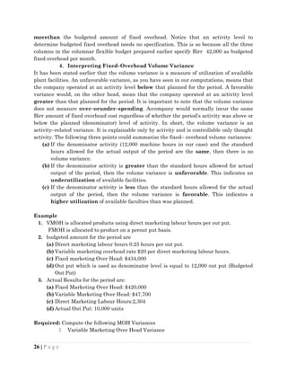
Variable Marketing Over Head Variance
26 | P a g e
27.
Fixed MarketingOver Head Variance
Prepare the necessary journal entries
CHAPTER THREE
VARIANCE: MIX, YIELD AND INVESTIGATION
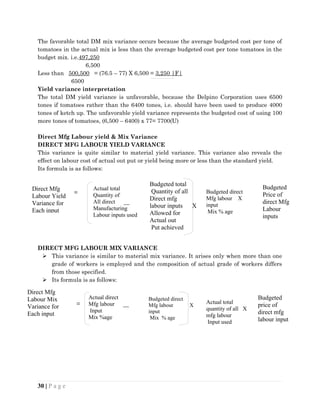
Direct Material Yield Variance
27 | P a g e
28.
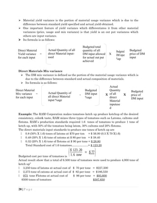
Material yieldvariance is the portion of material usage variance which is due to the
difference between standard yield specified and actual yield obtained.
One important feature of yield variance which differentiates it from other material
variances (price, usage and mix variance) is that yield is an out put variances which
others are input variance.
Its formula is as follows:
Direct Materials Mix variance
The DM mix variance is defined as the portion of the material usage variance which is
due to the difference between standard and actual composition of materials.
Its formula is as follows:
- X X
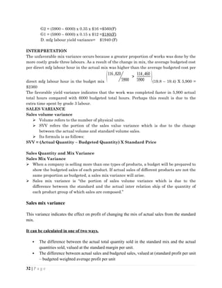
Example: The RAM Corporation makes tomatoes ketch up produce ketchup of the desired
consistency, color& taste, RAM mixes three types of tomatoes such as Latoms, caltoms and
flotoms. RAM`s production standards required 1.6 tones of tomatoes to produce 1 tone of
ketch up, with 50% of the tomatoes being latom, 30% caltoms and 20% flotoms.
The direct materials input standards to produce one tones of ketch up are
0.8 (50% X 1.6) tones of latoms at $70 per ton = $ 56.00 (0.5 X 70 X1.6)
0.48 (30% X 1.6) tone of catoms at $ 80 per ton = $ 38.40
0.32 (20% X 1.6) tone of flotoms at $ 90 per tone = $ 28.80
Total Standard cost of 1.6 tomatoes……………...= $ 123.20
Budgeted cost per tone of tomatoes is
($ 123.20
1.6 tone
= $ 77)
Actual result show that a total of 6.500 tone of tomatoes were used to produce 4,000 tone of
ketch up”
3,250 tons of latoms at actual cost of $ 70 per tone = $227,500
2,275 tone of catoms at actual cost of $ 82 per tone = $186,550
975 tone Flotoms at actual cost of $ 96 per tone = $93,600
6500 tones of tomatoes $507,650
28 | P a g e
Direct Material
Yield variance =
for each input
Actual Quantity of all
direct Material input-
used
Budgeted total
quantity of all
DM input allowed X
for actual out put
achieved
Budgeted
DM input
%age
Direct Material
Mix variance =
for each input
Actual Quantity of
all direct Material
input %age
Budgeted
DM input
%age
Budgeted
price of DM
input
Actual
Quantity
of all
direct
Material
inputuse
d
Budgeted
price of
DM input
29.
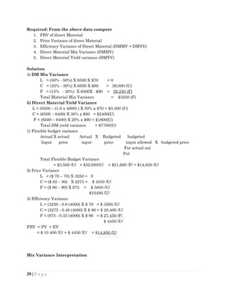
Required: From theabove data compute
1. FBV of direct Material
2. Price Variance of direct Material
3. Efficiency Variance of Direct Material (DMMV + DMYV)
4. Direct Material Mix Variance (DMMV)
5. Direct Material Yield variance (DMYV)
Solution
4) DM Mix Variance
L = (50% - 50%) X 6500 X $70 = 0
C = (35% - 30%) X 6500 X $80 = 26,000 (U)
F = (15% - 20%) X 6500X $90 = 29,250 (F)
Total Material Mix Variance = $3250 (F)
5) Direct Material Yield Variance
L = (6500 – (1.6 x 4000) ) X 50% x $70 = $3,500 (U)
C = (6500 – 6400) X 30% x $80 = $2400(U)
F = (6500 – 6400) X 20% x $90 = $1800(U)
Total DM yield variance = $7700(U)
1) Flexible budget variance
Actual X actual Actual X Budgeted budgeted
Input price input price input allowed X budgeted price
For actual out
Put
Total Flexible Budget Variance
= $3,500 /U/ + $32,950/U/ + $21,600 /F/ = $14,850 /U/
2) Price Variance
L = ($ 70 – 70) X 3250 = 0
C = ($ 82 – 80) X 2275 = $ 4550 /U/
F = ($ 96 – 90) X 975 = $ 5850 /U/
$10400 /U/
3) Efficiency Variance
L = (3250 - 0.8 (4000) X $ 70 = $ 3500 /U/
C = (2275 - 0.48 (4000) X $ 80 = $ 28,400 /U/
F = (975 - 0.32 (4000) X $ 90 = $ 27,450 /F/
$ 4450 /U/
FBV = PV + EV
= $ 10 400 /U/ + $ 4450 /U/ = $14,850 /U/
Mix Variance Interpretation
29 | P a g e
30.
The favorable totalDM mix variance occurs because the average budgeted cost per tone of
tomatoes in the actual mix is less than the average budgeted cost per tone tomatoes in the
budget mix. i.e.497,250
6,500
Less than 500,500 = (76.5 – 77) X 6,500 = 3,250 |F|
6500
Yield variance interpretation
The total DM yield variance is unfavorable, because the Delpino Corporation uses 6500
tones if tomatoes rather than the 6400 tones, i.e. should have been used to produce 4000
tones of ketch up. The unfavorable yield variance represents the budgeted cost of using 100
more tones of tomatoes, (6,500 – 6400) x 77= 7700(U)
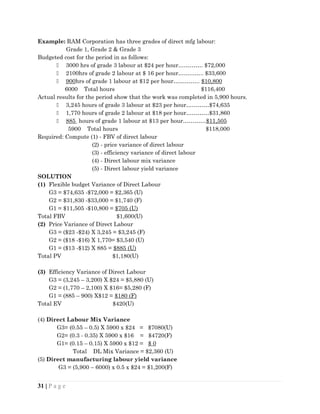
Direct Mfg Labour yield & Mix Variance
DIRECT MFG LABOUR YIELD VARIANCE
This variance is quite similar to material yield variance. This variance also reveals the
effect on labour cost of actual out put or yield being more or less than the standard yield.
Its formula is as follows:
=
DIRECT MFG LABOUR MIX VARIANCE
This variance is similar to material mix variance. It arises only when more than one
grade of workers is employed and the composition of actual grade of workers differs
from those specified.
Its formula is as follows:
=
30 | P a g e
Actual total
Quantity of
All direct __
Manufacturing
Labour inputs used
Budgeted total
Quantity of all
Direct mfg
labour inputs X
Allowed for
Actual out
Put achieved
Budgeted direct
Mfg labour X
input
Mix % age
Budgeted
Price of
direct Mfg
Labour
inputs
actual
Actual direct
Mfg labour __
Input
Mix %age
Budgeted direct
Mfg labour X
input
Mix % age
Budgeted
price of
direct mfg
labour input
Actual total
quantity of all X
mfg labour
Input used
Direct Mfg
Labour Yield
Variance for
Each input
Direct Mfg
Labour Mix
Variance for
Each input
31.
Example: RAM Corporationhas three grades of direct mfg labour:
Grade 1, Grade 2 & Grade 3
Budgeted cost for the period in as follows:
3000 hrs of grade 3 labour at $24 per hour…………. $72,000
2100hrs of grade 2 labour at $ 16 per hour……...….. $33,600
900hrs of grade 1 labour at $12 per hour………….. $10,800
6000 Total hours $116,400
Actual results for the period show that the work was completed in 5,900 hours.
3,245 hours of grade 3 labour at $23 per hour…………$74,635
1,770 hours of grade 2 labour at $18 per hour…………$31,860
885 hours of grade 1 labour at $13 per hour…………$11,505
5900 Total hours $118,000
Required: Compute (1) - FBV of direct labour
(2) - price variance of direct labour
(3) - efficiency variance of direct labour
(4) - Direct labour mix variance
(5) - Direct labour yield variance
SOLUTION
(1) Flexible budget Variance of Direct Labour
G3 = $74,635 -$72,000 = $2,365 (U)
G2 = $31,830 -$33,000 = $1,740 (F)
G1 = $11,505 -$10,800 = $705 (U)
Total FBV $1,600(U)
(2) Price Variance of Direct Labour
G3 = ($23 -$24) X 3,245 = $3,245 (F)
G2 = ($18 -$16) X 1,770= $3,540 (U)
G1 = ($13 -$12) X 885 = $885 (U)
Total PV $1,180(U)
(3) Efficiency Variance of Direct Labour
G3 = (3,245 – 3,200) X $24 = $5,880 (U)
G2 = (1,770 – 2,100) X $16= $5,280 (F)
G1 = (885 – 900) X$12 = $180 (F)
Total EV $420(U)
(4) Direct Labour Mix Variance
G3= (0.55 – 0.5) X 5900 x $24 = $7080(U)
G2= (0.3 - 0.35) X 5900 x $16 = $4720(F)
G1= (0.15 – 0.15) X 5900 x $12 = $ 0
Total DL Mix Variance = $2,360 (U)
(5) Direct manufacturing labour yield variance
G3 = (5,900 – 6000) x 0.5 x $24 = $1,200(F)
31 | P a g e
32.
G2 = (5900– 6000) x 0.35 x $16 =$560(F)
G1 = (5900 – 6000) x 0.15 x $12 =$180(F)
D. mfg labour yield variance= $1940 (F)
INTERPRETATION
The unfavorable mix variance occurs because a greater proportion of works was done by the
more costly grade three labours. As a result of the change in mix, the average budgeted cost
per direct mfg labour hour in the actual mix was higher than the average budgeted cost per
direct mfg labour hour in the budget mix
(116,820
5900
>
114,460
5900 )(19.8 – 19.4) X 5,900 =
$2360
The favorable yield variance indicates that the work was completed faster in 5,900 actual
total hours compared with 6000 budgeted total hours. Perhaps this result is due to the
extra time spent by grade 3 labour.
SALES VARIANCE
Sales volume variance
Volume refers to the number of physical units.
SVV refers the portion of the sales value variance which is due to the change
between the actual volume and standard volume sales.
Its formula is as follows:
SVV = (Actual Quantity – Budgeted Quantity) X Standard Price
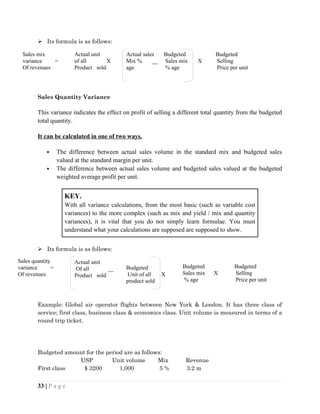
Sales Quantity and Mix Variance
Sales Mix Variance
When a company is selling more than one types of products, a budget will be prepared to
show the budgeted sales of each product. If actual sales of different products are not the
same proportion as budgeted, a sales mix variance will arise.
Sales mix variance is “the portion of sales volume variance which is due to the
difference between the standard and the actual inter relation ship of the quantity of
each product group of which sales are composed.”
Sales mix variance
This variance indicates the effect on profit of changing the mix of actual sales from the standard
mix.
It can be calculated in one of two ways.
The difference between the actual total quantity sold in the standard mix and the actual
quantities sold, valued at the standard margin per unit.
The difference between actual sales and budgeted sales, valued at (standard profit per unit
– budgeted weighted average profit per unit
32 | P a g e
33.
Its formulais as follows:
Sales Quantity Variance
This variance indicates the effect on profit of selling a different total quantity from the budgeted
total quantity.
It can be calculated in one of two ways.
The difference between actual sales volume in the standard mix and budgeted sales
valued at the standard margin per unit.
The difference between actual sales volume and budgeted sales valued at the budgeted
weighted average profit per unit.
KEY.
With all variance calculations, from the most basic (such as variable cost
variances) to the more complex (such as mix and yield / mix and quantity
variances), it is vital that you do not simply learn formulae. You must
understand what your calculations are supposed are supposed to show.
Its formula is as follows:
Example: Global air operator flights between New York & London. It has three class of
service; first class, business class & economics class. Unit volume is measured in terms of a
round trip ticket.
Budgeted amount for the period are as follows:
USP Unit volume Mix Revenue
First class $ 3200 1,000 5 % 3.2 m
33 | P a g e
Sales mix
variance =
Of revenues
Sales quantity
variance =
Of revenues
Actual unit
of all X
Product sold
Actual sales
Mix % __
age
Budgeted
Sales mix X
% age
Budgeted
Selling
Price per unit
Sales
mix
Budgeted
Unit of all X
product sold
Actual unit
Of all __
Product sold
Budgeted
Sales mix X
% age
Budgeted
Selling
Price per unit
34.
Business class $2400 3,000 15 % 7.2 m
Economic class $ 900 16,00080 %14.4 m
Total 20,000100%$ 24.8 m
Actual results for the period are as follows:
USPUnit volume Mix Revenue
First class 2,600 2,400 10% $6.24m
Business class 1,600 6,000 25% $9.6m
Economic class 70 15,60065%$10.92m
Total 24,000100%$26.76m
Required
1) Static budget variance = $1.96m (F)
2) FBV = 9.36m (U)
SVV = 11.32m (U)
3) Sales mix variance
4) Sales quantity variance
Solution
3) FC = 24,000 (10% - 5%) X 3,200 = 3.84m (F)
BC = 24,000 (25% - 15%) X 2,400 = 5.76m (F)
EC = 24,000 (65% - 80%) X 9,00 = 3.24m (U)
$ 6.36m (F)
Interpretation
A favorable sales mix variances arises at the individual product level when the actual sales
mix %age exceeds the budgeted sales mix % age (first class & BC). In constant economic
class has an unfavorable variance.
4) Sales quantity variance (SQV)
FC = (24,000 – 20,000) X 5% x $3,200 = $ 0.64m (F)
BC = (24,000 – 20,000) X 15% x $2400 = $1.44m (F)
EC = (24,000 – 20,000) X 80% x $900 = $ 2.88m (F)
$4.96m (F)
Interprétation
This variance is favorable when the actual unit of product sold exceeds the budget units of
product sold. Global sold 4000 more round trip ticket than was budgeted. Hence, its sales
quantity variance for revenue is favorable.
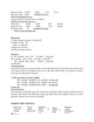
MARKET SIZE VARIANCE
34 | P a g e
Market size
variance in =
revenue
Actual
Market __
Size in unit
Budget
Market X
Share
Budgeted
average
Selling price
Per unit
Budgeted
Market X
Size in
unit
35.
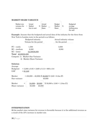
MARKET SHARE VARIANCE
Example:Assume that the budgeted and actual data of the industry for the three from
New York to London route in the period is as follows:
Budgeted industry Actual industry volume
Volume for the period for the period
FC – costly 1,500 3,000
BC – medium 6,000 9,000
EC – lower 32,50038,000
Total 40,00050,000
Compute: 1) Market Size Variance
2) Market Share Variance
Solution
Average
Budgeted = 3,200 x 0.05 + 2400 x 0.15 + 900 x 0.8
USP = $1,240
Market = (50,000 – 40,000) X 20,000 X 1240 = 6.2m (F)
Size variance 40,000
Market = 24,000– 20,000 X 50,000 x 1240 = 1.24m (U)
Share variance 50,000 40,000
INTERPRETATION
$6.2m market sizes variance for revenue is favorable because it is the additional revenue as
a result of the 25% increase in market size.
35 | P a g e
Actual
Market X
Size in unit
Actual
Market __
Share
Budget
Market X
Share
Market size
variance for =
revenue
Budgeted
average
Selling price
Per unit
36.
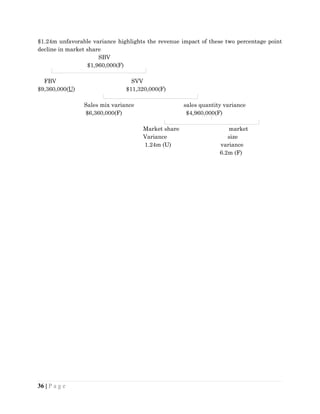
$1.24m unfavorable variancehighlights the revenue impact of these two percentage point
decline in market share
SBV
$1,960,000(F)
FBV SVV
$9,360,000(U) $11,320,000(F)
Sales mix variance sales quantity variance
$6,360,000(F) $4,960,000(F)
Market share market
Variance size
1.24m (U) variance
6.2m (F)
36 | P a g e

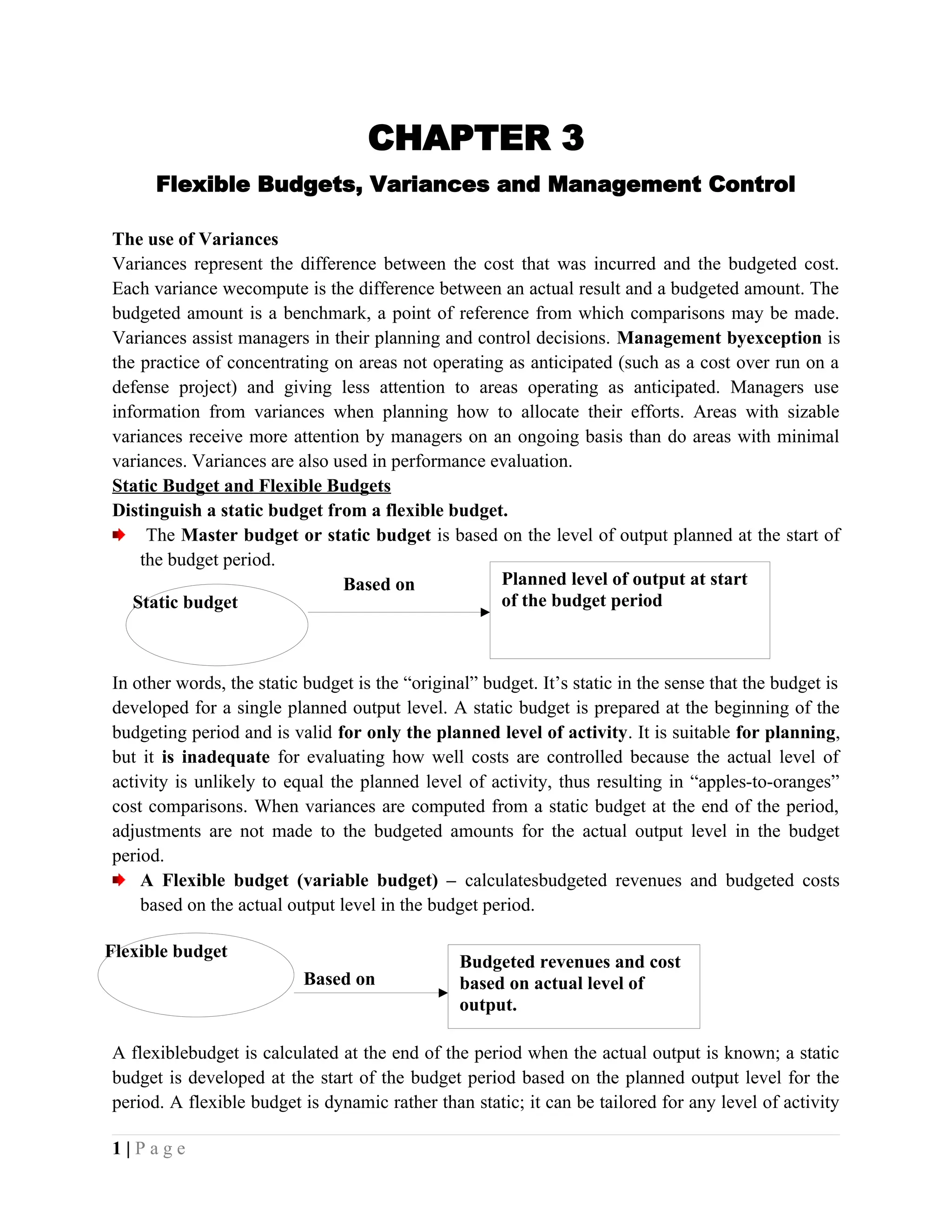
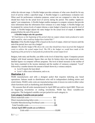
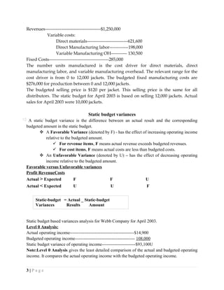
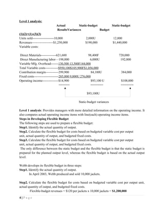
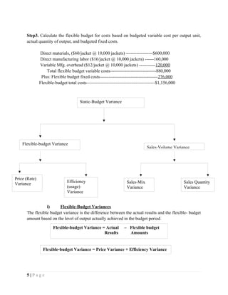
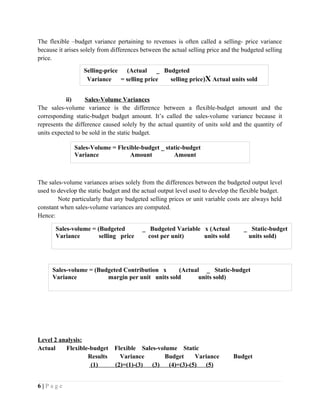
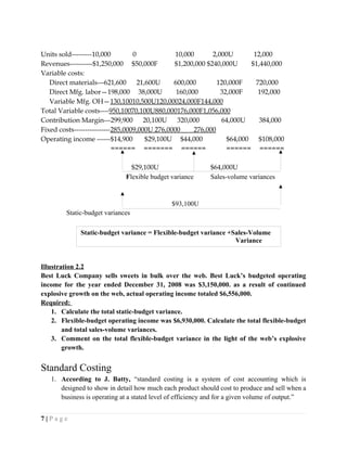
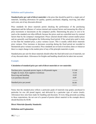
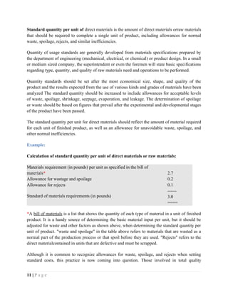
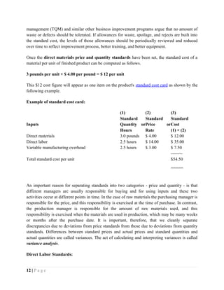
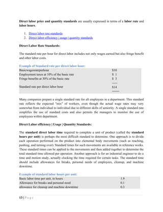
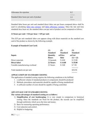
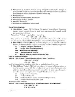
![If actual quantity used is less than the standard quantity, it will be favourable otherwise it
will be unfavourable or adverse.
Timing of Recognition of the Price Variance:
Some firms recognize the price variance for direct materials when the raw materials are
purchased, rather than waiting until the raw materials are put into production. In this
case, the AQ in the price variance will generally differ from the AQ in the quantity
variance, which is denoted in the following expressions for these variances:
PV = AQ Purchased x (AP – SP)
QV = SP x (AQ Used – SQ)
Where usually, AQ Purchased AQ Used
Recognizing the price variance when raw materials are purchased provides more timely
information to management about the cost of direct materials and the performance of the
purchasing department. Hence, this method for calculating the price variance has much to
commend it. However, in this situation, the sum of the price variance and quantity variance
will not equal the flexible budget variance, except by coincidence or when beginning and
ending quantities of raw materials are zero.
Direct Labour Variance
Labour Cost Variances: It is the difference between the standard direct wages given for the
activity and the actual wages paid. This variance arises due to change in wage rate or time
consumed or both. It can be calculated as follows:
Labour Cost Variance = Standard Cost ─ Actual Cost
= (SR x ST) ─ (AR x AT)
Labour Cost Variance is a sum total of labour rate variance, labour efficiency variance,
idle time variance and labour calendar variance
The formulas for splitting the flexible budget variance into a “price” variance and
“quantity” variance are the same for direct labor as direct materials. However, the
terminology differs slightly. What is called the price variance for direct materials is called
the rate variance or wage rate variance for direct labor.This variance measures any
deviation from standard in the average hourly rate paid to direct labor workers. In other
words, direct labor rate variance is the difference between the amount of actual hours
worked at actual rate and actual hours worked at standard rate.
[Labor rate variance = (Actual hours worked × Actual rate) − (Actual hours
worked × Standard rate)]
Or
LRV = AH (AR – SR)
16 | P a g e](https://image.slidesharecdn.com/costchapter3-1-250308115709-321c25c9/85/Cost-and-managerial-AccChapter-3-1-docx-16-320.jpg)
![Where AH; the actual labor hours used in production, AR isthe actual wage rate, and SR is
the budgeted wage rate.
Rates paid to the workers are usually predictable. Nevertheless, rate variances can arise
through the way labor is used. Skill workers with high hourly rates of pay may be given
duties that require little skill and call for low hourly rates of pay. This will result in an
unfavorable labor rate variance, since the actual hourly rate of pay will exceed the standard
rate specified for the particular task. In contrast, a favorable rate variance would result
when workers who are paid at a rate lower than specified in the standard are assigned to
the task. However, the low pay rate workers may not be as efficient. Finally, overtime work
at premium rates can be reason of an unfavorable labor price variance if the overtime
premium is charged to the labor account.
Who is responsible for the labor rate variance?
Since rate variances generally arise as a result of how labor is used, production supervisors
bear responsibility for seeing that labor price variances are kept under control.
Direct Labor Efficiency Variance
Definition and Explanation:
The quantity variance for direct labor is generally called direct labor efficiency
variance or direct labor usage variance. This variance measures the productivity of
labor time. No variance is more closely watched by management, since it is widely believed
that increasing the productivity of direct labor time is vital to reducing costs
What is called the quantity or usage variance for direct materials is called the efficiency
variance for direct labor. We abbreviate this variance as EV:
EV = SP x (AQ – SQ)
Or
[Labor efficiency variance = (Actual hours worked × Standard rate) − (Standard
hours allowed × Standard rate)]
Where SP and AQ are the same as above and SQ is the flexible budget quantity of labor
hours (the labor hours the factory should have used for the volume of output units
produced).
The issue discussed earlier in this chapter regarding the timing of the recognition of the
price variance for direct materials does not arise for direct labor. Consequently, for direct
labor, the sum of the wage rate variance and efficiency variance always equals the flexible
budget variance.
Assume the following additional data for Webb to illustrate price and efficiency variance
The standard direct manufacturing labor cost of a jacket at Webb.
Standard direct material cost per jacket: 2 square yards of cloth input allowed per output unit
(jacket) manufactured, at $30 standard price per square yard
Standard direct material cost per jacket = 2 square yards * $30 per square yard = $60
Standard direct manufacturing labor cost per jacket:0.8 manufacturing labor-hour of input
allowed per output unit manufactured, at $20 standard price per hour
Standard direct manufacturing labor cost per jacket = 0.8 labor-hour * $20 per labor-hour = $16
17 | P a g e](https://image.slidesharecdn.com/costchapter3-1-250308115709-321c25c9/85/Cost-and-managerial-AccChapter-3-1-docx-17-320.jpg)
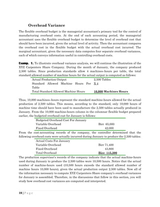
![The company’s total variable-overhead variance for January is computed below:
Actual Variable Overhead Birr 71,400
Budgeted Variable Overhead 65,000
Total Variable–Overhead Variance Birr 6,400 U
Variable Overhead Variance
What caused the company to spend Birr 6,400 more than the budgeted amount on variable
overhead? To discover the reasons behind this performance, the managerial accountant
computes the following variable overhead variances variable–overhead spending variance,
and variable–overhead efficiency variance.
Before we move in to the computation of these variances, carefully note the following
symbols:
AH = Actual hours (machine-hours in our case)
AR = Actual variable-overhand rate
SR = Standard variable-overhand rate
SH = Standard hours (machine hours in our case) allowed for actual output
1. Variable Overhead Spending Variance
The spending variance addresses the question, “How much should have been spent on
overhead, given the actual input?” It is a comparison of actual overhead with a flexible
budget based on actual hours.
To compute this variance, we use the formula given below:
SR
x
AH
OH
Variable
Actual
Variance
Spending
OH
Variable
Because actual variableoverhead is equal to actual hours (AH) times the actual variable
overhead rate (AR), the above formula could be rewritten as follows:
Variable−OH Spending Variance=[( AH x AR)−(AH x SR)]=AH x [ AR−SR]
Notice that the actual variable–overhead rate (AR) is computed using the formula giving
below.
AR=
Actual Variable OH
Actual Hours
The AR for the XYZ Carpenters Share Company is Birr 6.80 per machine hair as computed
below:
AR=
$71,400
10,500 Hours
=$6.80
Using the information at hand, let us now compute the variable-overheard spending
variance for the company.
Variable−OH Spending Variance=[ Actual Variable OH−(AH x SR)]
19 | P a g e](https://image.slidesharecdn.com/costchapter3-1-250308115709-321c25c9/85/Cost-and-managerial-AccChapter-3-1-docx-19-320.jpg)
![Variable−OH Spending Variance=[$ 71,400−(10,500 x $6.80)]=$3,150 Unfavourable
You can also apply the other formula given above to compute variable-overheard spending
variance for the company as indicated below:
Variable−OH Spending Variance=[( AH x AR)−(AH x SR)]=AH x [ AR−SR]
Variable−OH Spending Variance=[(10,500 x $6.80)−(10,500 x $6.50)]=$3,150 U
The variable-overhead spending variance is unfavorable because the actual variable-
overhead cost exceeded the expected amount, after adjusting that expectation for the actual
number of machine hours used or worked. Notice that the Birr 6.50 standard variable
overhead rate was calculated in our previous discussions under the topic “Flexible overhead
budget”
2. Variable–Overhead Efficiency Variance
The efficiency variance measures the amount of overhead variance attributable to using
more or less inputs than allowed by the standards, given the amount of production. If
actual hours worked are fewer than standard hours, the efficiency variance is favorable. An
unfavorable variance occurs when actual hours exceed standard hours. To compute this
variance, we use the formula given below:
Variable−OH Efficiency Variance=[( AH x SR )−(SH x SR)]
XYZ Carpenter Share Company’s variable- overhead efficient variance for January is
computed as follows:
Variable−OH Efficiency Variance=[(10,500 x $6.80)−(10,000 x $6.50)]=$3,250 U
The above formula can be simplified by expressing it in factored from as follows:
Variable−OH Efficiency Variance=SR x [AH−SH]
The variable-overhead efficiency variance is unfavorable because actual machine hours
(10,500 hours) exceeded the standard allowed machine hours (10,000 hours) for the actual
output (2,500 tables) manufactured in January. Now carefully observe that, as shown
below, the total variable –overhead variance is the sum of the variable – overhead spending
and efficiency variances:
Variable–Overhead Spending Variance Birr 3,150 U
Variable–Overhead Efficiency Variance 3,250 U
Total Variable–Overhead Variance Birr 6,400 U
The variable–overhead spending variance measures the aggregate effect of differences
between the actual variable–overhead rate and the standard efficiency variance, in
contrast, measures the aggregate effect of differences between the actual activity base and
the standard activity base allowed for the actual out put achieved. Recall that the activity
base in the XYZ Carpenters Share Company problem is machine hours. A summary of
variable variances is presented in the table that follows. Notice, in this table, that “hours”
represent machine hours and rates per “hour” stand to indicate rates per machine hour.
20 | P a g e](https://image.slidesharecdn.com/costchapter3-1-250308115709-321c25c9/85/Cost-and-managerial-AccChapter-3-1-docx-20-320.jpg)
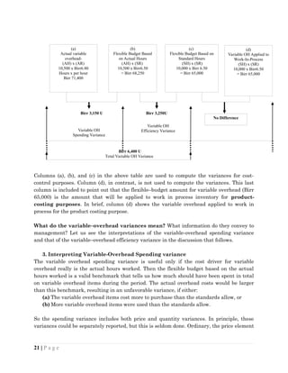
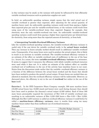
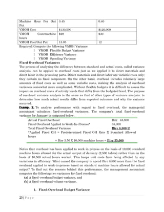
![The budget variance is the difference between the actual fixed overhead costs incurred
during the period and the budgeted fixed overhead costs as contained in the flexible
overhead budget. This variance, used by managers to control fixed overhead costs, and that
is computed by using the following formula:
Fixed−OH Budget Variance=[ Actual Variable OH Cost−Flexible Budget Fixed OH Cost]
XYZ Carpenters Share Company’s fixed-overhead budget variance for January is, applying
the formula given about, computed as follows:
Fixed−OH Budget Variance=[ Actual Variable OH Cost−Flexible Budget Fixed OH Cost]
Fixed−OH Budget Variance=[$ 43,800−$ 42,000]=$1,800 Unfavourable
2. Fixed-Overhead Volume Variance
The volume variance is a measure of utilization of plant facilities. The variance arises
whenever the standard hours allowed for the actual output of a period are different from
the dominator activity level that was planned when the period began. This variance can
be commuted using any one of the following two formulas:
Fixed OH Volume Variance=[Predeter mined FOH Rate(Denominators Hrs−Standard Hrs Allowed)]
Fixed OH Volume Variance=[Flexibe Budget FOH Cost−Applied FOH]
Let’s now compute the fixed –overhead volume variance for the XYZ Carpenters Share
Company’s problem, using the above two formulas.
Fixed OH Volume Variance=[Pr edeter mined FOH Rate(Denominators Hrs−S tandard Hrs Allowed)]
Fixed OH Volume Variance=[$ 3.50(12,000 Hrs−10,000 Hrs )]=$7,000 Unfaourable
Notice that, to compute the predetermined overhead rate for XYZ Carpenters Share
Company, 12,000 machine-hours per month was taken as planned activity when the
period began. Using this base, recall that, the predetermined fixed overhead rate was
computed to be Birr 3.50 per machine hour as follows:
Predetermined Fixed overhead rate =
Flexible budget fixed overhead cost
Denominator activity
=
$42,000
12,000 Hrs
=$3.50
The budgeted activity level for the moth (12,000 machine hours) is used as the denominator
activity in the formula for the predetermined overhead rate. These 12,000 machine hours
are what we called denominator hours in the formula for volume variance. In general,
the estimated total units in the base (machine hours, direct-labor hours, etc.) in the formula
for the predetermined overhead rate are the denominator activity. Once an estimated
activity level (denominator activity) has been chosen, it remains unchanged throughout the
year even if the actual activity turns out to be different from what was estimated. The
reason for not changing the denominator is to maintain stability in the amount of overhead
applied to each unit of product regardless of when it is produced during the year.
24 | P a g e](https://image.slidesharecdn.com/costchapter3-1-250308115709-321c25c9/85/Cost-and-managerial-AccChapter-3-1-docx-24-320.jpg)
![Birr 8,800 unfavorable
Total Fixed–OH variance
Actual Fixed OH Cost
Birr 43,800
Flexible Budget
Fixed OHCost
Birr 42,000
Fixed OHCost Applied to Work-In-Process10,000 standard hours X Birr 3.50 per hours
= Birr 35,000
Birr 1,800 Unfavorable
Fixed–OH
Budget variance
Birr 7,000 Unfavorable
Fixed– OH
Volume variance
U
Recall that 10,000 machine hours represent the standard hours allowed for actual output of
January (2,500 tables) at 4 standard machine hours per table. You can as well arrive at the
same result of fixed overhead volume variance applying the second formula as shown below:
Fixed OH Volume Variance=[$ 42,000−$35,000]=$7,000 Unfavourable
Now carefully observe that, as shown blow, the total fixed-overhead variance is the sum of
the fixed-overhead budget and volume variances:
Fixed-Overhead Budget Variance Birr 1,800 U
Fixed–Overhead Volume Variance 4,000 U
Total Fixed Overhead Variance Birr 8,800 U
A summary of fixed–overhead variance is presented in the table that follows.
The fixed–Overhead variances convey useful information to management. Let’s see, in the
discussion that follows, at the interpretation of these variances.
3. Interpreting Fixed–Overhead Budget Variance
The budget variance is the real control variance for fixed overhead, because it compares
actual expenditures with budgeted fixed – overhead costs. The budget variances for fixed
overhead can be very useful, since they represent the difference between how much should
have been spent (according to the flexible overhead budget) and how much was actually
spent. An unfavorable fixed – overhead budget variance calls for an explanation of why it
happened. If, for instance, the production supervisor’s salary shows an unfavorable budget
variance, it could be due to many reasons. The reasons could be an increase in salaries,
overtime work, or another supervisor could have been hired. Proper explanation should be
given as to why another supervisor was hired, if this was not included in the budget when
activity for the period was planned. In brief, the fixed – overhead budget variance for XYZ
Carpenters Share Company’s problem is unfavorable, because the company spent
25 | P a g e](https://image.slidesharecdn.com/costchapter3-1-250308115709-321c25c9/85/Cost-and-managerial-AccChapter-3-1-docx-25-320.jpg)