Download to read offline


![�
�
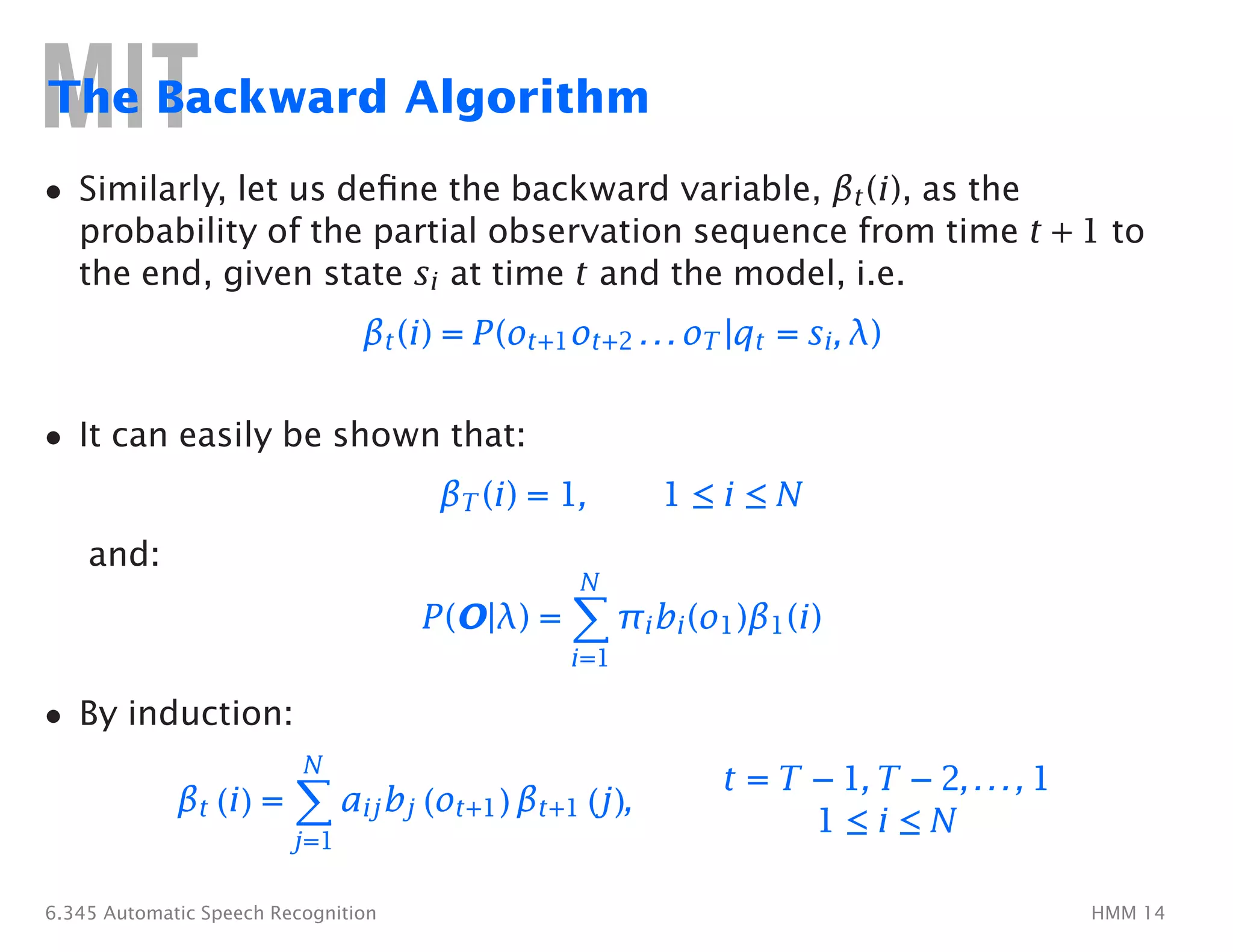
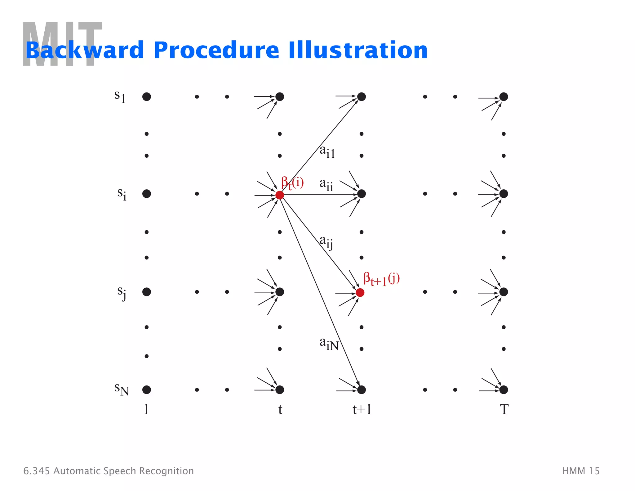
The Forward Algorithm
• Let us define the forward variable, αt(i), as the probability of the
partial observation sequence up to time t and�state si at time t,
given the model, i.e.
αt(i) = P(o1o2 . . . ot, qt = si|λ)
• It can easily be shown that:
α1(i) = πibi(o1), 1 ≤ i ≤ N
N
P(O|λ) = αT (i)
• By induction: i=1
N
1 ≤ t ≤ T − 1
αt+1 (j) = [ αt (i) aij]bj (ot+1),
1 ≤ j ≤ N
i=1
• Calculation is on the order of N2T.
For N = 5, T = 100 ⇒ 100 · 52 computations, instead of 1072
6.345 Automatic Speech Recognition HMM 12](https://image.slidesharecdn.com/continioushmm-220814143624-302a20de/75/continious-hmm-pdf-12-2048.jpg)


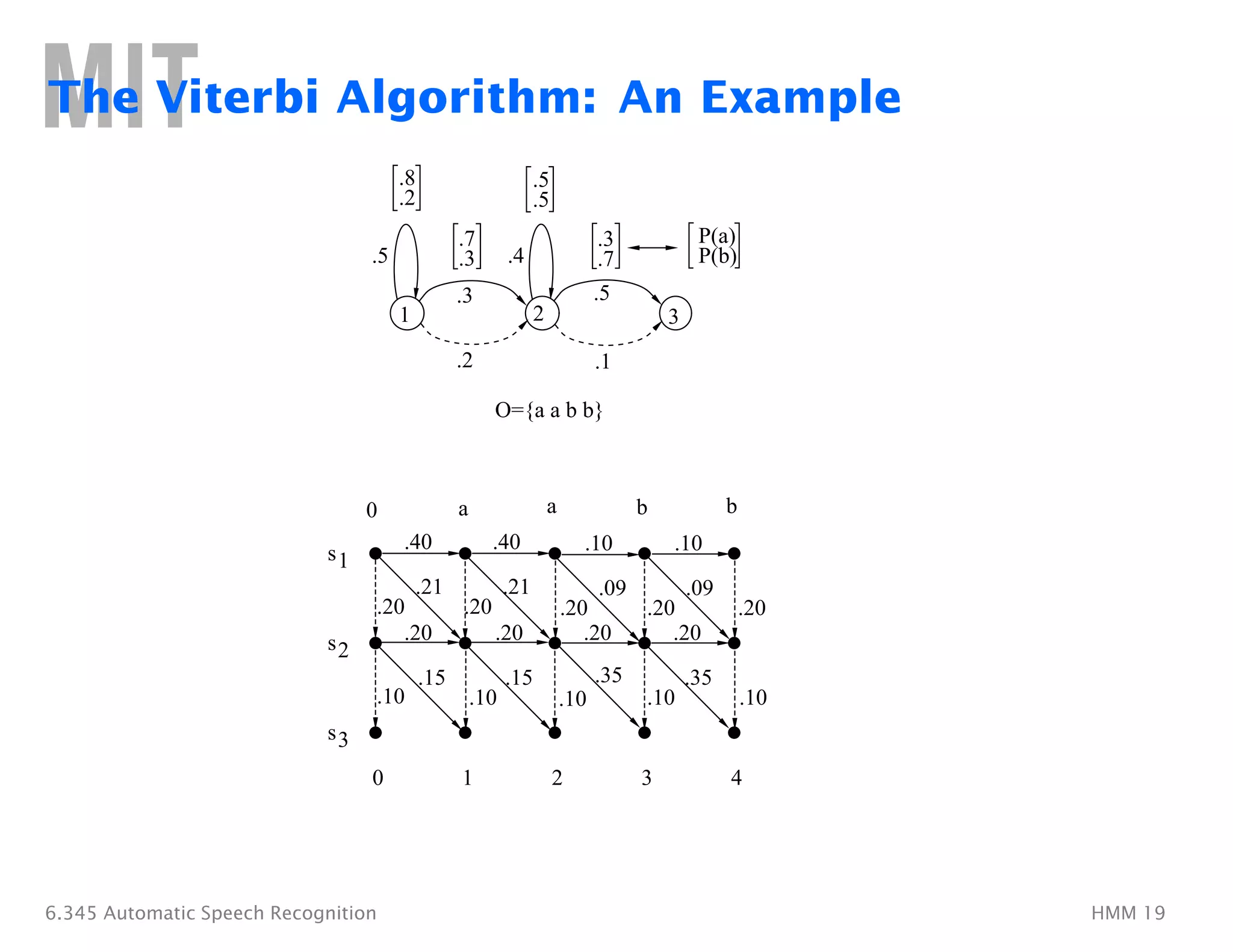
![i
Finding Optimal State Sequences
• The individual optimality criterion has the problem that the
optimum state sequence may not obey state transition constraints
• Another optimality criterion is to choose the state sequence which
maximizes P(Q, O|λ); This can be found by the Viterbi algorithm
• Let us define δt(i)�as the highest probability along a single path, at
time t, which accounts for the first t observations, i.e.
δt(i) = � max� P(q1q2�. . . qt−1, qt =�si, o1o2�. . . ot|λ)
q1,q2,...,qt−1�
• By induction: δt+1(j) = [max�δt(i)aij]bj(ot+1)�
• To retrieve the state sequence, we must keep track of the state
sequence which gave the best path, at time t, to state si
– We do this in a separate array ψt(i)�
6.345 Automatic Speech Recognition HMM 17](https://image.slidesharecdn.com/continioushmm-220814143624-302a20de/75/continious-hmm-pdf-17-2048.jpg)
![T
The Viterbi Algorithm
1. Initialization:
δ1(i) = �
πibi(o1), 1�≤ i ≤ N
ψ1(i) = 0�
2. Recursion:
δt(j) = �
max�
1≤i≤N
[δt−1(i)aij]bj(ot), 2�≤ t ≤ T 1�≤ j ≤ N
ψt(j)� =�argmax[δt−1(i)aij], 2�≤ t ≤ T 1�≤ j ≤ N
1≤i≤N
3. Termination:
P∗ = max�
1≤i≤N
[δT (i)]�
q∗
=�argmax[δT (i)]
1≤i≤N
4. Path (state-sequence) backtracking:
qt
∗
=�ψt+1(qt
∗
+1), t =�T − 1, T − 2, . . . , 1�
Computation ≈ N2T
6.345 Automatic Speech Recognition HMM 18](https://image.slidesharecdn.com/continioushmm-220814143624-302a20de/75/continious-hmm-pdf-18-2048.jpg)


![�
�
Continuous Density Hidden Markov Models
• A continuous density HMM replaces the discrete observation
probabilities, bj(k), by a continuous PDF bj(x)
• A common practice is to represent bj(x) as a mixture of Gaussians:
M
bj(x) = cjkN[x, µjk, Σjk] 1 ≤ j ≤ N
k=1
where cjk is the mixture weight
M
cjk ≥ 0 (1 ≤ j ≤ N, 1 ≤ k ≤ M, and cjk = 1, 1 ≤ j ≤ N),
k=1
N is the normal density, and
µjk and Σjk are the mean vector and covariance matrix
associated with state j and mixture k.
6.345 Automatic Speech Recognition HMM 30](https://image.slidesharecdn.com/continioushmm-220814143624-302a20de/75/continious-hmm-pdf-30-2048.jpg)


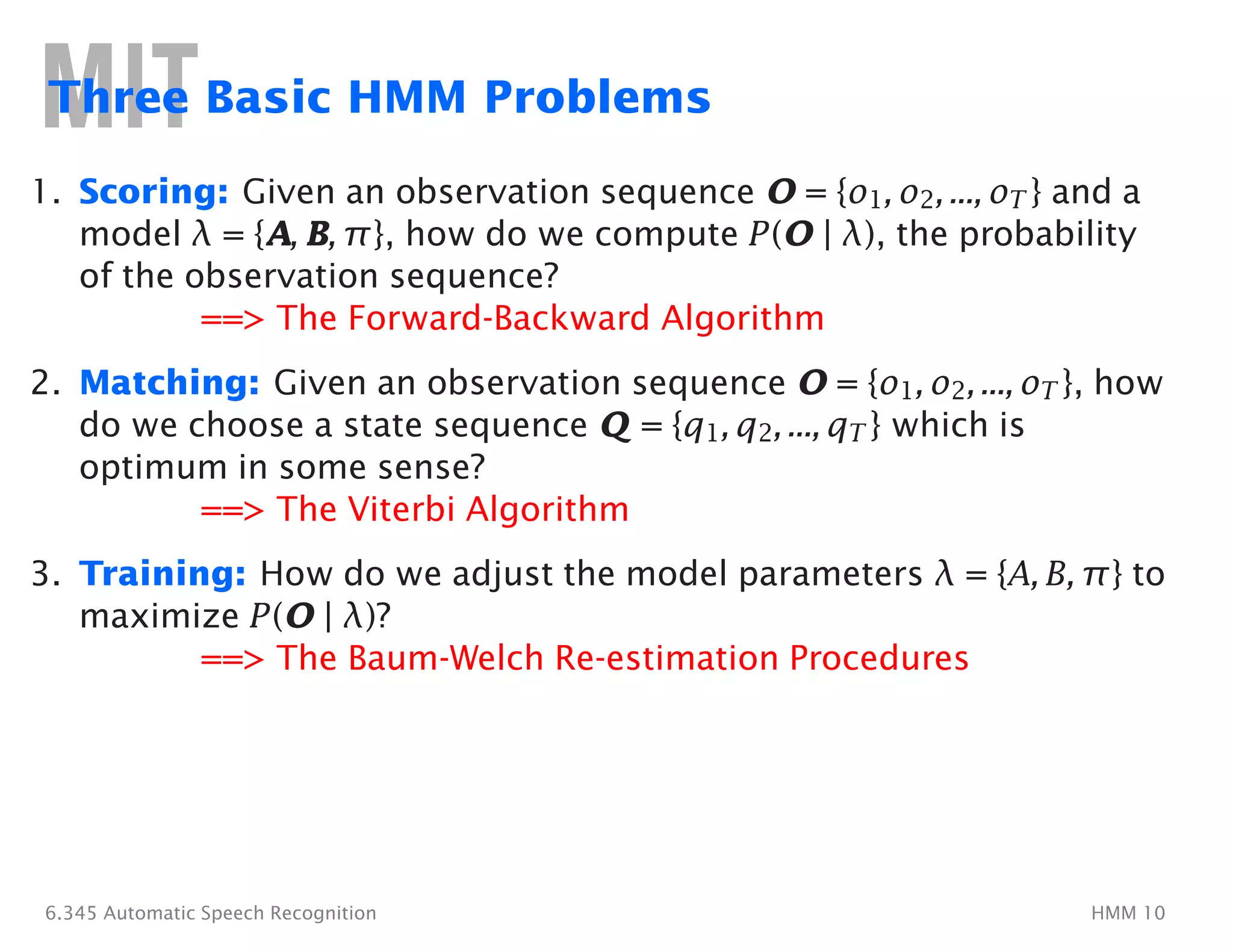
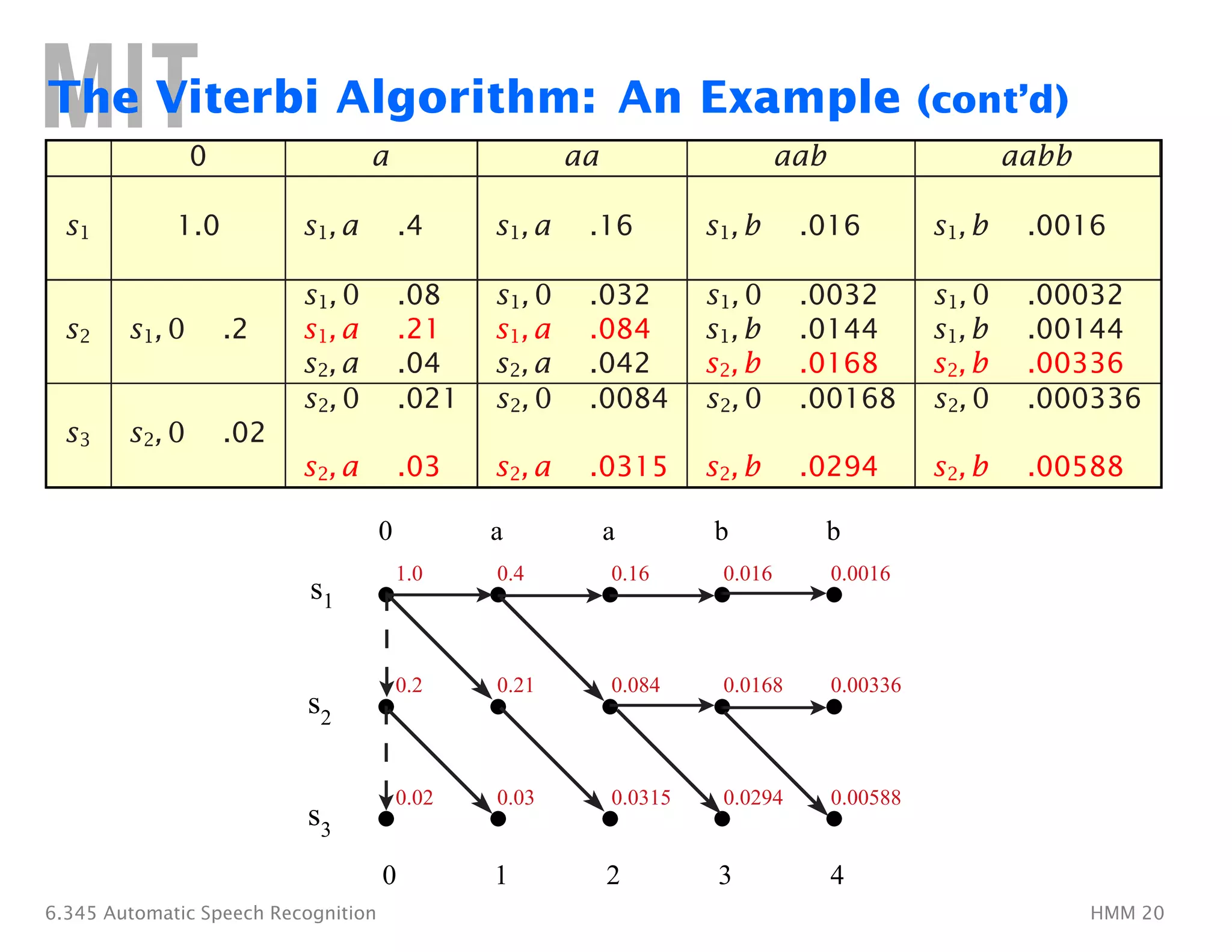
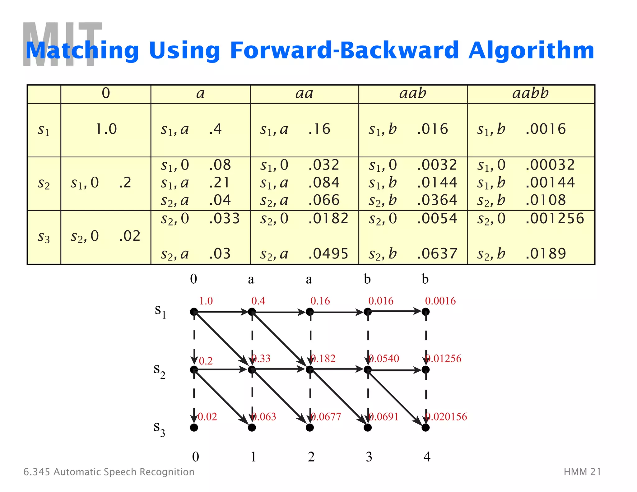
The document discusses Hidden Markov Models (HMMs) and their application to automatic speech recognition. It covers the three main problems in HMMs - scoring, matching, and training. Scoring involves computing the probability of an observation sequence given a model. Matching finds the optimal state sequence. Training adjusts the model parameters to maximize the likelihood of observation sequences. The Forward-Backward and Viterbi algorithms are described as solutions to scoring and matching respectively.


![129966864599036360[1]](https://cdn.slidesharecdn.com/ss_thumbnails/1299668645990363601-130806105150-phpapp01-thumbnail.jpg?width=640&height=640&fit=bounds)


