Computer Aided Design and Manufacturing.pdf

(i)
PUBLICATIONS
TECHNICAL
An Up-Thrust for Knowledge
®
SINCE 1993
SUBJECT CODE : ME8691
Strictly as per Revised Syllabus of
Anna University
Choice Based Credit System (CBCS)
Semester - VI (MECH)
Computer Aided Design
& Manufacturing
A. Jacob Moses
M.E. (Ph.D.)
Assistant Professor,
Department of Mechanical Engineering,
Loyola-ICAM College of Engineering & Technology (LICET),
Chennai
Anup Goel
B.E. Mechanical
Post Graduation in Tool Design with CAD/CAM
Managing Director of AG Engineering Study Centre,
Akurdi, Pune
13 Years Teaching Experience
Renjin J. Bright
M.E. (Ph.D.)
Assistant Professor,
Department of Mechanical Engineering,
National Engineering College, Kovilpatti
Ruchi Agarwal
B.E. (MECH), GATE Qualified

(ii)
AU 17
9 [1]
788194382515
ã Copyright with Authors
All publishing rights reserved with . No part of this book
should be reproduced in any form, Electronic, Mechanical, Photocopy or any information storage and
retrieval system without prior permission in writing, from Technical Publications, Pune.
(printed and ebook version) Technical Publications
Printer :
Yogiraj Printers & Binders
Sr.No. 10/1A,
Ghule Industrial Estate, Nanded Village Road,
Tal. - Haveli, Dist. - Pune - 411041.
Published by :
Amit Residency, Office No.1, 412, Shaniwar Peth, Pune - 411030, M.S. INDIA
Ph.: +91-020-24495496/97, Telefax : +91-020-24495497
Email : sales@technicalpublications.org Website : www.technicalpublications.org
PUBLICATIONS
TECHNICAL
An Up-Thrust for Knowledge
®
SINCE 1993
ISBN 978-81-943825-1-5
Price : 395/-
`
9 7 8 8 1 9 4 3 8 2 5 1 5
Semester - VI (Mechanical Engineering)
Subject Code : ME8691
Computer Aided Design
& Manufacturing
First Edition : January 2020

Preface
The importance of Computer Aided Design and Manufacturing is well known in
various engineering fields. Overwhelming response to our books on various subjects
inspired us to write this book. The book is structured to cover the key aspects of the
subject Computer Aided Design and Manufacturing.
The book uses plain, lucid language to explain fundamentals of this subject. The
book provides logical method of explaining various complicated concepts and stepwise
methods to explain the important topics. Each chapter is well supported with necessary
illustrations, practical examples and solved problems. All the chapters in the book are
arranged in a proper sequence that permits each topic to build upon earlier studies. All
care has been taken to make students comfortable in understanding the basic concepts
of the subject.
Representative questions have been added at the end of each Chapter to help the
students in picking important points from that Chapter.
The book not only covers the entire scope of the subject but explains the philosophy
of the subject. This makes the understanding of this subject more clear and makes it
more interesting. The book will be very useful not only to the students but also to the
subject teachers. The students have to omit nothing and possibly have to cover nothing
more.
We wish to express our profound thanks to all those who helped in making this
book a reality. Much needed moral support and encouragement is provided on
numerous occasions by our whole family. We wish to thank the Publisher and the
entire team of Technical Publications who have taken immense pain to get this book
in time with quality printing.
Any suggestion for the improvement of the book will be acknowledged and well
appreciated.
Authors
Anup Goel
A. Jacob Moses
Renjin J. Bright
Ruchi Agarwal
Dedicated to Family, Friends & Dear Students
(iii)

Syllabus
Computer Aided Design and Manufacturing
[ME8691]
Unit I Introduction
Product cycle- Design process- sequential and concurrent engineering - Computer aided design
- CAD system architecture- Computer graphics - co-ordinate systems - 2D and 3D
transformations- homogeneous coordinates - Line drawing - Clipping - viewing
transformation-Brief introduction to CAD and CAM - Manufacturing Planning, Manufacturing
control- Introduction to CAD/CAM - CAD/CAM concepts - Types of production - Manufacturing
models and Metrics - Mathematical models of Production Performance. (Chapter - 1)
Unit II Geometric Modeling
Representation of curves - Hermite curve- Bezier curve - B-spline curves-rational
curves-Techniques for surface modeling - surface patch- Coons and bicubic patches - Bezier
and B-spline surfaces. Solid modeling techniques - CSG and B-rep. (Chapter - 2)
Unit III CAD Standards
Standards for computer graphics - Graphical Kernel System (GKS) - standards for exchange
images - Open Graphics Library (OpenGL) - Data exchange standards - IGES, STEP, CALS etc. -
communication standards. (Chapter - 3)
Unit IV Fundamental of CNC and Part Programing
Introduction to NC systems and CNC - Machine axis and Co-ordinate system - CNC machine
tools- Principle of operation CNC- Construction features including structure- Drives and CNC
controllers- 2D and 3D machining on CNC- Introduction of Part Programming, types - Detailed
Manual part programming on Lathe & Milling machines using G codes and M codes - Cutting
Cycles, Loops, Sub program and Macros- Introduction of CAM package. (Chapter - 4)
Unit V Cellular Manufacturing and Flexible
Manufacturing System (FMS)
Group Technology(GT),Part Families - Parts Classification and coding - Simple Problems in
Opitz Part Coding system - Production flow Analysis - Cellular Manufacturing - Composite part
concept - Types of Flexibility - FMS - FMS Components - FMS Application & Benefits - FMS
Planning and Control - Quantitative analysis in FMS. (Chapter - 5)
(iv)

Table of Contents
Unit - I
Chapter - 1 Introduction (1 - 1) to (1 - 116)
1.1 Introduction to CAD...........................................................................................1 - 2
1.2 Product Cycle.....................................................................................................1 - 2
1.3 Design Process...................................................................................................1 - 5
1.4 Sequential and Concurrent Engineering............................................................1 - 8
1.5 Computer Aided Design (CAD).........................................................................1 - 12
1.6 CAD System Architecture.................................................................................1 - 15
1.7 Computer Graphics..........................................................................................1 - 16
1.8 Coordinate System ..........................................................................................1 - 18
1.9 2D Transformations.........................................................................................1 - 20
1.9.1 Homogeneous Coordinates . . . . . . . . . . . . . . . . . . . . . . . . . . . . . . . . . . . . . . . . . 1 - 27
1.9.2 Solved Examples on 2D Transformation . . . . . . . . . . . . . . . . . . . . . . . . . . . . . . . 1 - 29
1.10 3D Transformations.......................................................................................1 - 51
1.11 Line Drawing..................................................................................................1 - 52
1.11.1 DDA Algorithm. . . . . . . . . . . . . . . . . . . . . . . . . . . . . . . . . . . . . . . . . . . . . . . . . . . 1 - 53
1.11.2 Bresenham's Line Drawing Algorithm . . . . . . . . . . . . . . . . . . . . . . . . . . . . . . . . 1 - 55
1.11.3 Solved Examples on DDA Algorithm and Bresenham's Algorithm. . . . . . . . . . 1 - 57
1.12 Clipping..........................................................................................................1 - 62
1.13 Viewing Transformation ................................................................................1 - 69
1.14 Brief Introduction to CAD and CAM..............................................................1 - 71
1.14.1 Computer Aided Design (CAD) . . . . . . . . . . . . . . . . . . . . . . . . . . . . . . . . . . . . . . 1 - 71
1.15 Computer Aided Manufacturing (CAM).........................................................1 - 77
1.15.1 CAD-CAM Integration . . . . . . . . . . . . . . . . . . . . . . . . . . . . . . . . . . . . . . . . . . . . . 1 - 77
1.15.2 Manufacturing Planning . . . . . . . . . . . . . . . . . . . . . . . . . . . . . . . . . . . . . . . . . . . 1 - 78
(v)

1.15.3 Manufacturing Control . . . . . . . . . . . . . . . . . . . . . . . . . . . . . . . . . . . . . . . . . . . . 1 - 79
1.16 Types of Production Systems.........................................................................1 - 80
1.17 Manufacturing Models and Metrics..............................................................1 - 84
1.17.1 Production Performance Measures . . . . . . . . . . . . . . . . . . . . . . . . . . . . . . . . . . 1 - 85
1.17.2 Manufacturing Costs . . . . . . . . . . . . . . . . . . . . . . . . . . . . . . . . . . . . . . . . . . . . . . 1 - 96
1.18 Break Even Analysis - A Tool for Manufacturing Control.............................1 - 100
Review Questions ............................................................................................... 1 - 103
Part A : Two Marks Question with Answers .................................................. 1 - 104
Part B : University Questions ........................................................................ 1 - 114
Unit - II
Chapter - 2 Geometric Modeling (2 - 1) to (2 - 48)
2.1 Introduction...................................................................................................... 2 - 3
2.2 Methods of Geometric Modeling ..................................................................... 2 - 3
2.2.1 Wire Frame Modeling. . . . . . . . . . . . . . . . . . . . . . . . . . . . . . . . . . . . . . . . . . . . . . . 2 - 4
2.2.2.1 Advantages and Disadvantages of Wire Frame Modeling . . . . . . . . . 2 - 7
2.3 Representation of Curves ................................................................................ 2 - 8
2.4 Parametric and Non-parametric Curves........................................................... 2 - 9
2.5 Order of Continuity......................................................................................... 2 - 11
2.6 Interpolation and Approximation of Curve..................................................... 2 - 12
2.6.1 Difference between Interpolation Curve and Approximation Curve . . . . . . . . 2 - 12
2.7 Hermite Cubic Curve....................................................................................... 2 - 13
2.7.1 Solved Examples on Hermite Cubic Curve . . . . . . . . . . . . . . . . . . . . . . . . . . . . . 2 - 15
2.8 Bezier Curve.................................................................................................... 2 - 18
2.8.1 Solved Examples on Bezier Curve . . . . . . . . . . . . . . . . . . . . . . . . . . . . . . . . . . . . 2 - 20
2.9 B-Spline Curve ................................................................................................ 2 - 22
2.9.1 Difference between Hermite Cubic Spline, Bezier Wave and B-Spline Curve . 2 - 23
2.10 Rational Curve............................................................................................... 2 - 23
2.11 Surface Modeling ......................................................................................... 2 - 24
(vi)

2.11.1 Classification of Surfaces in Geometric Modeling . . . . . . . . . . . . . . . . . . . . . . 2 - 24
2.11.2 Blending Function . . . . . . . . . . . . . . . . . . . . . . . . . . . . . . . . . . . . . . . . . . . . . . . 2 - 26
2.12 Parametrization of Surface Patch ................................................................. 2 - 27
2.12.1 Bicubic Patches . . . . . . . . . . . . . . . . . . . . . . . . . . . . . . . . . . . . . . . . . . . . . . . . . 2 - 28
2.13 Bezier Surface ............................................................................................... 2 - 28
2.14 B-spline Surface ........................................................................................... 2 - 29
2.15 Boolean Operation........................................................................................ 2 - 30
2.16 Solid Modeling ............................................................................................. 2 - 31
2.17 Constructive Solid Geometry ....................................................................... 2 - 33
2.18 Boundary Representation ............................................................................ 2 - 35
2.18.1 Different between C-rep Modeling and B-rep Modeling . . . . . . . . . . . . . . . . 2 - 35
2.19 Cell Consumption ......................................................................................... 2 - 36
2.20 Spatial Occupancy Enumeration .................................................................. 2 - 36
2.21 Sweep Representation.................................................................................. 2 - 37
Part A : Two Marks Questions with Answers .................................................. 2 - 38
Part B : University Questions with Answers .................................................... 2 - 43
Unit - III
Chapter - 3 CAD Standards (3 - 1) to (3 - 40)
3.1 Introduction...................................................................................................... 3 - 2
3.2 Standards for Computer Graphics .................................................................... 3 - 4
3.2.1 Graphics Kernel System (GKS) . . . . . . . . . . . . . . . . . . . . . . . . . . . . . . . . . . . . . . . . 3 - 5
3.3 Standards for Exchange of Images.................................................................. 3 - 10
3.3.1 Open Graphics Library (OpenGL). . . . . . . . . . . . . . . . . . . . . . . . . . . . . . . . . . . . . 3 - 10
3.4 Data Exchange Standards ............................................................................... 3 - 13
3.4.1 IGES - Initial Graphics Exchange Specification . . . . . . . . . . . . . . . . . . . . . . . . . . 3 - 13
3.4.2 STEP - Standard for the Exchange of Product Data . . . . . . . . . . . . . . . . . . . . . . 3 - 18
3.4.3 CALS - Continuous Acquisition and Life-Cycle Support . . . . . . . . . . . . . . . . . . . 3 - 20
(vii)

3.4.4 PDES - Product Data Exchange Specification . . . . . . . . . . . . . . . . . . . . . . . . . . . 3 - 23
3.4.5 DXF (Data Exchange Format) . . . . . . . . . . . . . . . . . . . . . . . . . . . . . . . . . . . . . . . . 3 - 24
3.5 Communication Standards ............................................................................. 3 - 26
3.5.1 Local Area Networks. . . . . . . . . . . . . . . . . . . . . . . . . . . . . . . . . . . . . . . . . . . . . . . 3 - 27
3.5.2 Wide Area Networks . . . . . . . . . . . . . . . . . . . . . . . . . . . . . . . . . . . . . . . . . . . . . . 3 - 28
3.5.3 Levels of Communication Standards. . . . . . . . . . . . . . . . . . . . . . . . . . . . . . . . . . 3 - 30
Review Questions ................................................................................................ 3 - 31
Part A : Two Marks Questions with Answers................................................... 3 - 32
Unit - IV
Chapter - 4 Fundamental of CNC and Part Programming
(4 - 1) to (4 - 118)
4.1 Introduction...................................................................................................... 4 - 3
4.2 Numerical Control............................................................................................. 4 - 3
4.2.1 Basic Elements of NC System. . . . . . . . . . . . . . . . . . . . . . . . . . . . . . . . . . . . . . . . . 4 - 4
4.3 Classification of NC System .............................................................................. 4 - 7
4.3.1 According to Tool Positioning . . . . . . . . . . . . . . . . . . . . . . . . . . . . . . . . . . . . . . . . 4 - 7
4.3.1.1 Comparison of Absolute and Incremental System. . . . . . . . . . . . . 4 - 8
4.3.2 According to Motion Control System . . . . . . . . . . . . . . . . . . . . . . . . . . . . . . . . . . 4 - 8
4.3.3 According to Servo Control System. . . . . . . . . . . . . . . . . . . . . . . . . . . . . . . . . . . 4 - 10
4.3.3.1 Comparison of Open Loop and Closed Loop System . . . . . . . . . . . 4 - 11
4.3.4 According to Feedback Devices . . . . . . . . . . . . . . . . . . . . . . . . . . . . . . . . . . . . . 4 - 11
4.4 Advantages of NC System............................................................................... 4 - 12
4.5 Disadvantages of NC System .......................................................................... 4 - 12
4.6 Applications of NC System.............................................................................. 4 - 12
4.7 Types of Numerical Control System................................................................ 4 - 13
4.8 Conventional Numerical Control (NC) ............................................................ 4 - 13
4.9 Direct Numerical Control (DNC)...................................................................... 4 - 13
(viii)

4.10 Computerized Numerical Control (CNC)....................................................... 4 - 14
4.11 Constructional Features of CNC Machines ................................................... 4 - 15
4.11.1 Machine Structure . . . . . . . . . . . . . . . . . . . . . . . . . . . . . . . . . . . . . . . . . . . . . . . 4 - 16
4.11.2 Drives. . . . . . . . . . . . . . . . . . . . . . . . . . . . . . . . . . . . . . . . . . . . . . . . . . . . . . . . . . 4 - 17
4.11.3 Actuation System . . . . . . . . . . . . . . . . . . . . . . . . . . . . . . . . . . . . . . . . . . . . . . . . 4 - 18
4.11.4 Slideways for Machines . . . . . . . . . . . . . . . . . . . . . . . . . . . . . . . . . . . . . . . . . . . 4 - 21
4.11.5 Automatic Tool Changer (ATC) . . . . . . . . . . . . . . . . . . . . . . . . . . . . . . . . . . . . . 4 - 24
4.11.6 Automatic Pallet Changer (APC) . . . . . . . . . . . . . . . . . . . . . . . . . . . . . . . . . . . . 4 - 25
4.11.7 Transducers/Control Elements . . . . . . . . . . . . . . . . . . . . . . . . . . . . . . . . . . . . . 4 - 27
4.11.8 Feedback Devices . . . . . . . . . . . . . . . . . . . . . . . . . . . . . . . . . . . . . . . . . . . . . . . . 4 - 27
4.12 Advantages and Disadvantages of CNC Machines ....................................... 4 - 28
4.13 Comparison between NC, CNC and DNC System ......................................... 4 - 29
4.14 Adaptive Control System (ACS) .................................................................... 4 - 30
4.15 Machining Centre ......................................................................................... 4 - 31
4.15.1 Horizontal Machining Centre (HMC) . . . . . . . . . . . . . . . . . . . . . . . . . . . . . . . . 4 - 32
4.15.2 Vertical Machining Centre (VMC) . . . . . . . . . . . . . . . . . . . . . . . . . . . . . . . . . . 4 - 32
4.16 Program Reader ........................................................................................... 4 - 34
4.17 New Trends in Tool Materials ..................................................................... 4 - 34
4.18 Tool Inserts .................................................................................................. 4 - 35
4.19 Work Holding in CNC Machines .................................................................. 4 - 36
4.20 Axis Nomenclature for CNC Machines ......................................................... 4 - 36
4.21 Part Programming ........................................................................................ 4 - 39
4.21.1 Manual Part Programming. . . . . . . . . . . . . . . . . . . . . . . . . . . . . . . . . . . . . . . . . 4 - 39
4.21.2 Preparatory Functions . . . . . . . . . . . . . . . . . . . . . . . . . . . . . . . . . . . . . . . . . . . . 4 - 43
4.22 Procedure to Write a Part Program ............................................................. 4 - 49
4.23 Part Programming for Lathe ........................................................................ 4 - 50
4.24 Part Programming for Milling and Drilling ................................................... 4 - 67
4.25 Subroutine ................................................................................................... 4 - 90
(ix)

4.26 Canned Cycle ................................................................................................ 4 - 93
4.26.1 Comparison between Subroutine and Canned Cycle . . . . . . . . . . . . . . . . . . . 4 - 93
4.26.2 Slot Milling (G74) . . . . . . . . . . . . . . . . . . . . . . . . . . . . . . . . . . . . . . . . . . . . . . . . 4 - 93
4.26.3 Rectangular Pocket Milling (G75) . . . . . . . . . . . . . . . . . . . . . . . . . . . . . . . . . . . 4 - 95
4.27 Automatically Programmed Tools (APT) ...................................................... 4 - 96
4.27.1 Structure of APT . . . . . . . . . . . . . . . . . . . . . . . . . . . . . . . . . . . . . . . . . . . . . . . . . 4 - 96
4.28 Micromachining ........................................................................................... 4 - 99
4.28.1 Wafer Machining . . . . . . . . . . . . . . . . . . . . . . . . . . . . . . . . . . . . . . . . . . . . . . . . 4 - 99
4.29 Part Programming using APT ..................................................................... 4 - 100
4.30 Introduction of CAM Package .................................................................... 4 - 107
Part A : Two Marks Questions with Answers ................................................ 4 - 111
Unit - V
Chapter - 5 Cellular Manufacturing and Flexible
Manufacturing System (FMS) (5 - 1) to (5 - 54)
5.1 Group Technology ............................................................................................ 5 - 3
5.1.1 Benefits of Group Technology . . . . . . . . . . . . . . . . . . . . . . . . . . . . . . . . . . . . . . . 5 - 3
5.2 Part Families .................................................................................................... 5 - 3
5.2.1 Identification of Part Families . . . . . . . . . . . . . . . . . . . . . . . . . . . . . . . . . . . . . . . . 5 - 4
5.2.1.1 Visual Inspection Method . . . . . . . . . . . . . . . . . . . . . . . 5 - 4
5.2.1.2 Parts Classification and Coding . . . . . . . . . . . . . . . . . . . . 5 - 5
5.2.1.3 Production Flow Analysis . . . . . . . . . . . . . . . . . . . . . . . 5 - 5
5.3 Parts Classification and Coding......................................................................... 5 - 5
5.3.1 Part Design Attributes . . . . . . . . . . . . . . . . . . . . . . . . . . . . . . . . . . . . . . . . . . . . . . 5 - 5
5.3.2 Part Manufacturing Attributes. . . . . . . . . . . . . . . . . . . . . . . . . . . . . . . . . . . . . . . . 5 - 5
5.4 Structures used for Classifying and Coding the Parts ..................................... 5 - 5
5.4.1 Hierarchical Structure . . . . . . . . . . . . . . . . . . . . . . . . . . . . . . . . . . . . . . . . . . . . . . 5 - 5
5.4.2 Chain-type Structure . . . . . . . . . . . . . . . . . . . . . . . . . . . . . . . . . . . . . . . . . . . . . . . 5 - 6
5.4.3 Mixed Mode Symbol . . . . . . . . . . . . . . . . . . . . . . . . . . . . . . . . . . . . . . . . . . . . . . . . 5 - 6
(x)

5.5 OPTIZ Coding System ....................................................................................... 5 - 6
5.5.1 Solved Examples of Optiz Part Coding System . . . . . . . . . . . . . . . . . . . . . . . . . . 5 - 8
5.6 Production Flow Analysis ............................................................................... 5 - 10
5.6.1 Production Flow Analysis (PFA) Procedure . . . . . . . . . . . . . . . . . . . . . . . . . . . . 5 - 10
5.6.1.1 Data Collection . . . . . . . . . . . . . . . . . . . . . . . . . . . 5 - 11
5.6.1.2 Sortation of Process Routings . . . . . . . . . . . . . . . . . . . . 5 - 12
5.6.1.3 PFA Chart . . . . . . . . . . . . . . . . . . . . . . . . . . . . . 5 - 12
5.6.1.4 Cluster Analysis . . . . . . . . . . . . . . . . . . . . . . . . . . 5 - 13
5.7 Rank Order Clustering..................................................................................... 5 - 13
5.7.1 Advantage of PFA . . . . . . . . . . . . . . . . . . . . . . . . . . . . . . . . . . . . . . . . . . . . . . . . . 5 - 19
5.7.2 Disadvantage of PFA. . . . . . . . . . . . . . . . . . . . . . . . . . . . . . . . . . . . . . . . . . . . . . . 5 - 19
5.8 Cellular Manufacturing .................................................................................. 5 - 19
5.8.1 Objective of Cellular Manufacturing . . . . . . . . . . . . . . . . . . . . . . . . . . . . . . . . . 5 - 19
5.9 Machine Cell Design ....................................................................................... 5 - 20
5.9.1 Types of Machine Cell. . . . . . . . . . . . . . . . . . . . . . . . . . . . . . . . . . . . . . . . . . . . . . 5 - 20
5.9.1.1 Single Machines . . . . . . . . . . . . . . . . . . . . . . . . . . 5 - 20
5.9.1.2 Group Machine Cell with Manual Handling . . . . . . . . . . . . . . . 5 - 20
5.9.1.3 Group Machine Cell with Semi-integrated Handling . . . . . . . . . . . 5 - 20
5.9.1.4 Flexible Manufacturing Cell or Flexible Manufacturing System (FMS) . . . . 5 - 20
5.9.2 Types of Layout. . . . . . . . . . . . . . . . . . . . . . . . . . . . . . . . . . . . . . . . . . . . . . . . . . . 5 - 21
5.9.2.1 Inline Layout . . . . . . . . . . . . . . . . . . . . . . . . . . . 5 - 21
5.9.2.2 Loop Layout . . . . . . . . . . . . . . . . . . . . . . . . . . . . 5 - 22
5.9.2.3 Rectangular Layout . . . . . . . . . . . . . . . . . . . . . . . . . 5 - 22
5.10 Part Movement between the Cell ................................................................ 5 - 23
5.11 Key Machine ................................................................................................ 5 - 24
5.12 Composite Part Concept............................................................................... 5 - 24
5.13 Flexible Manufacturing System (FMS).......................................................... 5 - 25
5.13.1 Flexibility Tests . . . . . . . . . . . . . . . . . . . . . . . . . . . . . . . . . . . . . . . . . . . . . . . . . . 5 - 25
(xi)

5.14 Types of Flexibility ....................................................................................... 5 - 26
5.14.1 Single Machine Cell. . . . . . . . . . . . . . . . . . . . . . . . . . . . . . . . . . . . . . . . . . . . . . . 5 - 27
5.14.2 Flexible Manufacturing Cell (FMC) . . . . . . . . . . . . . . . . . . . . . . . . . . . . . . . . . . 5 - 28
5.14.3 Flexible Manufacturing System (FMS) . . . . . . . . . . . . . . . . . . . . . . . . . . . . . . . 5 - 28
5.14.4 Difference between FMC and FMS . . . . . . . . . . . . . . . . . . . . . . . . . . . . . . . . . . 5 - 29
5.15 Level of Flexibility ........................................................................................ 5 - 30
5.15.1 Dedicated FMS . . . . . . . . . . . . . . . . . . . . . . . . . . . . . . . . . . . . . . . . . . . . . . . . . . 5 - 30
5.15.2 Random Order FMS . . . . . . . . . . . . . . . . . . . . . . . . . . . . . . . . . . . . . . . . . . . . . . 5 - 30
5.16 Components of FMS ..................................................................................... 5 - 31
5.16.1 Work Stations . . . . . . . . . . . . . . . . . . . . . . . . . . . . . . . . . . . . . . . . . . . . . . . . . . . 5 - 31
5.16.1.1 Load / Unload Work Stations . . . . . . . . . . . . . . . . . . . . 5 - 31
5.16.1.2 Machining Work Stations . . . . . . . . . . . . . . . . . . . . . . 5 - 32
5.16.1.3 Assembly Work Stations . . . . . . . . . . . . . . . . . . . . . . 5 - 32
5.16.1.4 Supporting Work Stations. . . . . . . . . . . . . . . . . . . . . . 5 - 32
5.16.1.5 Other work stations . . . . . . . . . . . . . . . . . . . . . . . . 5 - 32
5.16.2 Material Handling and Storage System. . . . . . . . . . . . . . . . . . . . . . . . . . . . . . . 5 - 33
5.16.2.1 FMS Layout Configurations . . . . . . . . . . . . . . . . . . . . . 5 - 33
5.16.3 Computer Control System . . . . . . . . . . . . . . . . . . . . . . . . . . . . . . . . . . . . . . . . . 5 - 38
5.16.4 Human Resources. . . . . . . . . . . . . . . . . . . . . . . . . . . . . . . . . . . . . . . . . . . . . . . . 5 - 39
5.17 Applications of FMS ...................................................................................... 5 - 39
5.18 Advanages of FMS ........................................................................................ 5 - 40
5.19 FMS Planning and Control ........................................................................... 5 - 41
5.19.1 FMS Planning Issues . . . . . . . . . . . . . . . . . . . . . . . . . . . . . . . . . . . . . . . . . . . . . 5 - 41
5.19.2 FMS Design Issues . . . . . . . . . . . . . . . . . . . . . . . . . . . . . . . . . . . . . . . . . . . . . . . 5 - 41
5.19.3 FMS Operational Issues . . . . . . . . . . . . . . . . . . . . . . . . . . . . . . . . . . . . . . . . . . . 5 - 42
5.20 Quantitative Analysis in FMS ........................................................................ 5 - 43
5.20.1 Bottle Neck Model . . . . . . . . . . . . . . . . . . . . . . . . . . . . . . . . . . . . . . . . . . . . . . 5 - 43
Part A : Two Marks Questions with Answers................................................... 5 - 49
Solved Model Question Paper ...................................................... (M - 1) to (M - 4)
(xii)

Syllabus : Product cycle- Design process- sequential and concurrent engineering-
Computer aided design – CAD system architecture- Computer graphics –
co-ordinate systems- 2D and 3D transformations- homogeneous coordinates -
Line drawing -Clipping- viewing transformation-Brief introduction to CAD
and CAM – Manufacturing Planning, Manufacturing control- Introduction to
CAD/CAM –CAD/CAM concepts ––Types of production - Manufacturing
models and Metrics – Mathematical models of Production Performance
Section No. Topic Name Page No.
1.1 Introduction to CAD 1 - 2
1.2 Product Cycle 1 - 2
1.3 Design Process 1 - 5
1.4 Sequential and Concurrent Engineering 1 - 8
1.5 Computer Aided Design (CAD) 1 - 12
1.6 CAD System Architecture 1 - 15
1.7 Computer Graphics 1 - 16
1.8 Coordinate System 1 - 18
1.9 2D Transformations 1 - 20
1.10 3D Transformations 1 - 51
1.11 Line Drawing 1 - 52
1.12 Clipping 1 - 62
1.13 Viewing Transformation 1 - 69
1.14 Brief Introduction to CAD and CAM 1 - 71
1.15 Computer Aided Manufacturing (CAM) 1 - 77
1.16 Types of Production Systems 1 - 80
1.17 Manufacturing Models and Metrics 1 - 84
1.18 Break Even Analysis - A Tool for Manufacturing Control 1 - 100
Part A : Two Marks Question with Answers 1 - 104
Part B : University Questions with Answers 1 - 114
1 - 1 Computer Aided Design and Manufacturing
Chapter - 1
Introduction
Unit - I

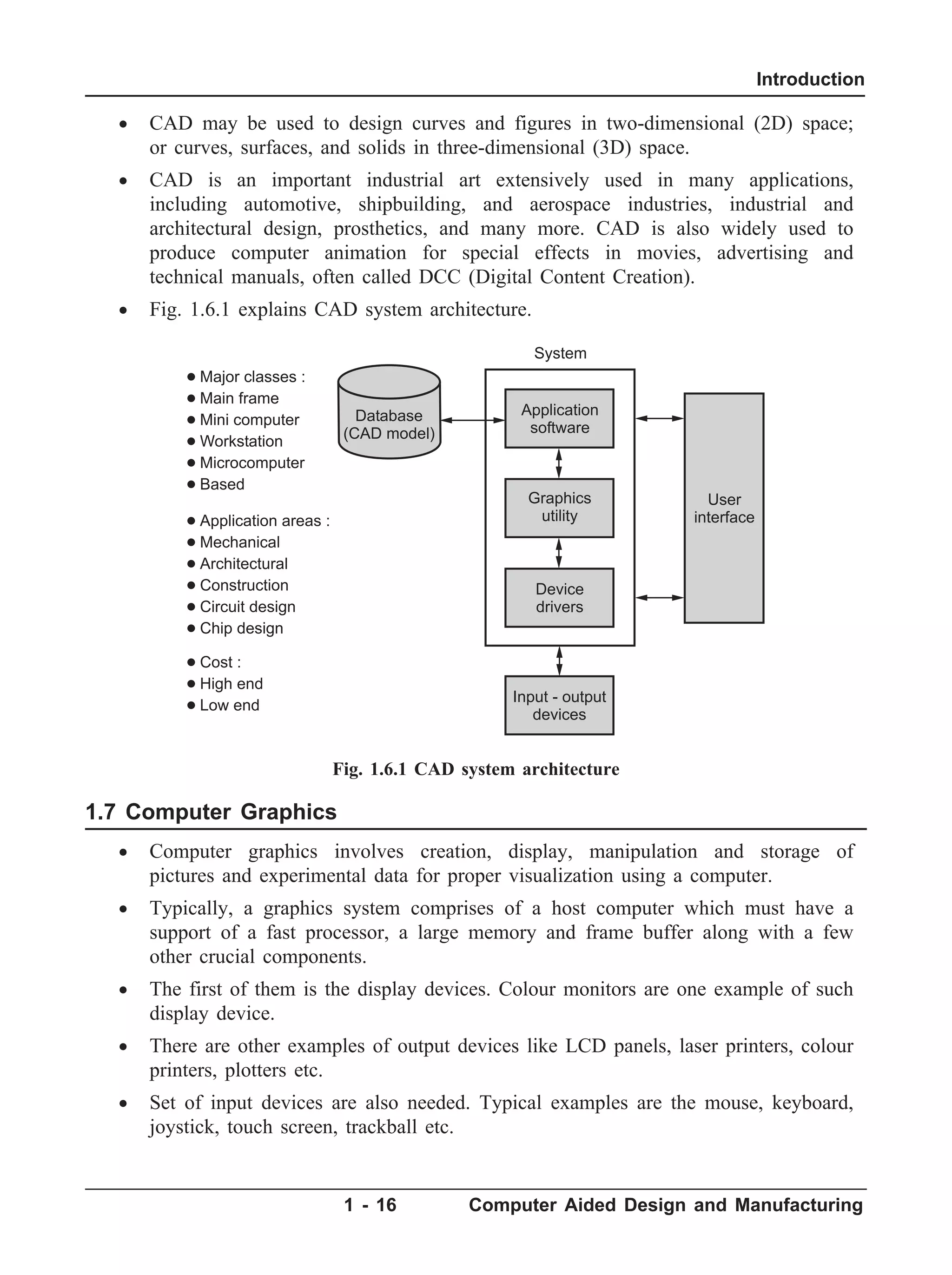
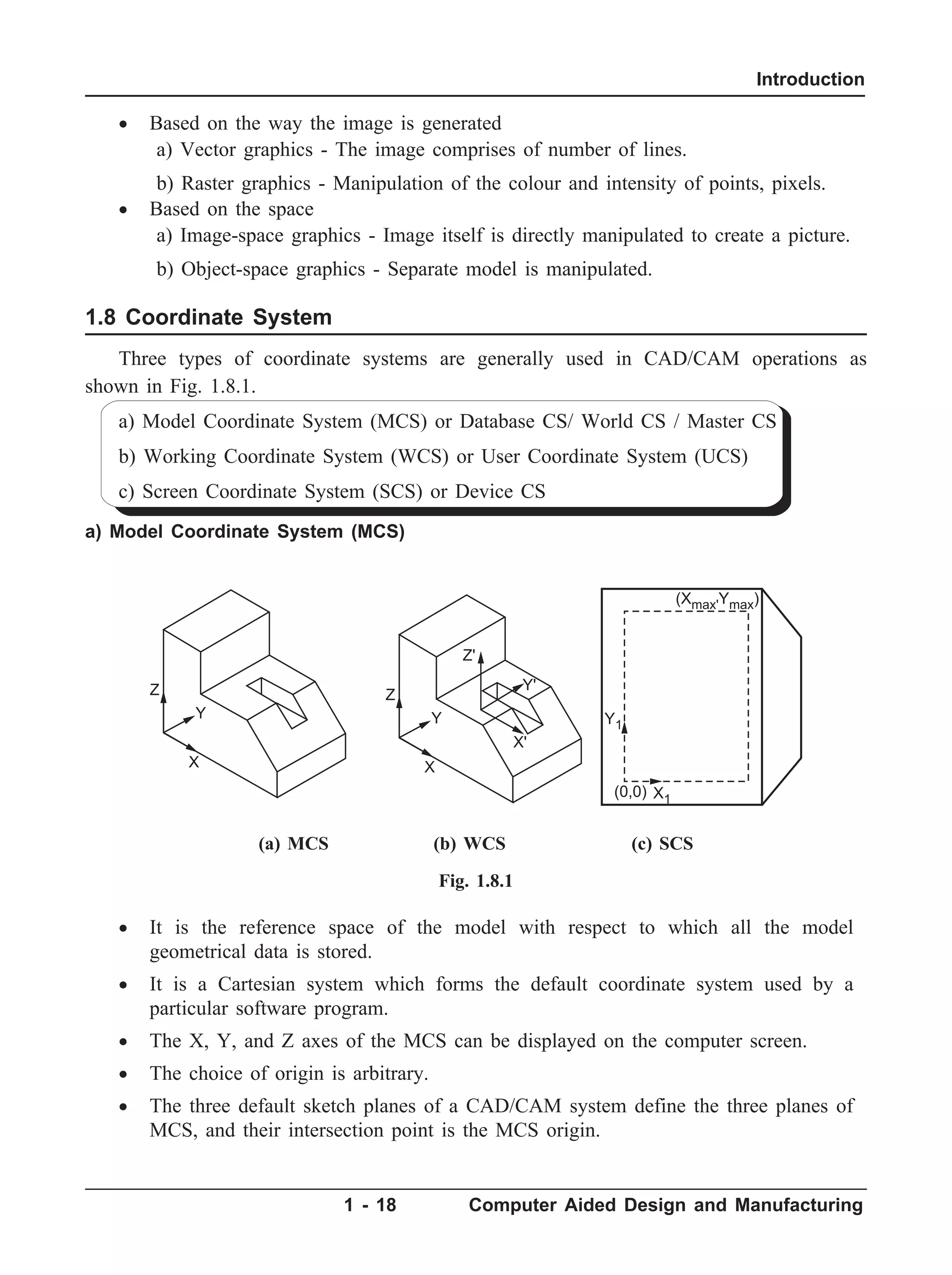
1.1 Introduction to CAD
· CAD (Computer Aided Design) is the use of computer software to design and
document a product's design process.
· Engineering drawing entails the use of graphical symbols such as points, lines,
curves, planes and shapes.
· Essentially, it gives detailed description about any component in a graphical form.
· The use of orthographic projections was formally introduced by the French
mathematician Gaspard Monge in the eighteenth century.
· Since visual objects transcend languages, engineering drawings have evolved and
become popular over the years.
· While earlier engineering drawings were handmade, studies have shown that
engineering designs are quite complicated.
· A solution to many engineering problems requires a combination of organization,
analysis, problem solving principles and a graphical representation of the
problem.
· Objects in engineering are represented by a technical drawing (also called as
drafting) that represents designs and specifications of the physical object and data
relationships.
· CAD is used to design, develop and optimize products.
· While it is very versatile, CAD is extensively used in the design of tools and
equipment required in the manufacturing process as well as in the construction
domain.
· CAD enables design engineers to layout and to develop their work on a computer
screen, print and save it for future editing.
· When it was introduced first, CAD was not exactly an economic proposition
because the machines at those times were very costly.
· The increasing computer power in the later part of the twentieth century, with the
arrival of minicomputer and subsequently the microprocessor, has allowed
engineers to use CAD files that are an accurate representation of the
dimensions / properties of the object.
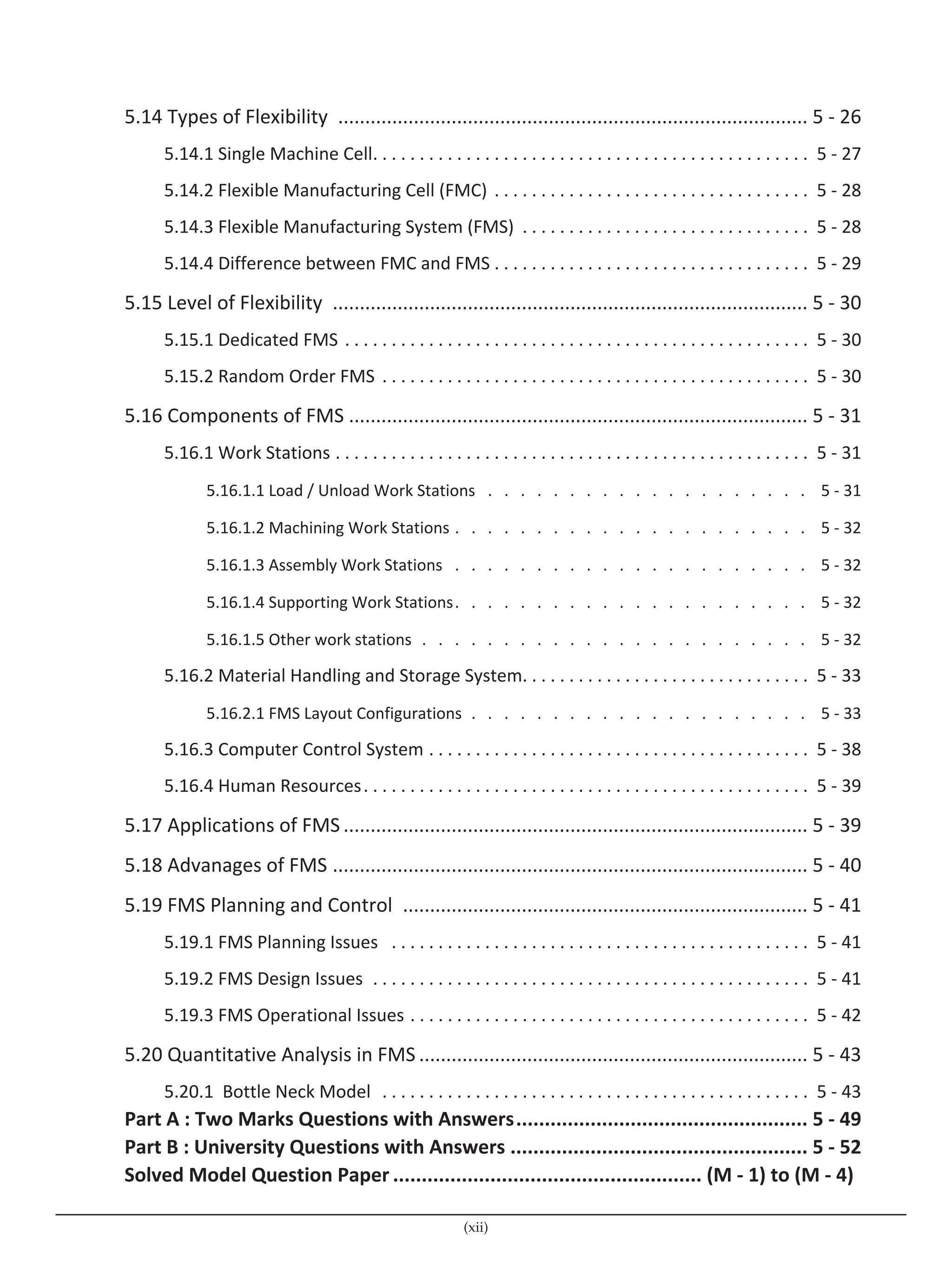
1.2 Product Cycle + [AU : Dec.-18]
· In the design and manufacture of a product various activities and functions must
be accomplished. These activities and functions are referred to as the
"Product Cycle".
· The product cycle includes all the activities starting from identification for
product to deliver the finished product to the customer. Fig. 1.2.1 explains
various stages in product life cycle. Fig. 1.2.2 depicts various steps in the product
cycle and Fig. 1.2.3 explains product cycle in in a detailed manner.
Introduction

· Two main processes in the product cycle are :
i) Design process
ii) Manufacturing process.
i) Design process
· The activities involved in the design process can be classified into :
· Synthesis
· Analysis.
Introduction
Sales
Introduction Growth
The 4 life cycle stages and their marketing implications
Maturity Decline
· Low sales · Increasing sales · Peak sales · Falling sales
· High cost per
customer
· Cost per customer falls · Cost per customer
lowest
· Cost per customer low
· Financial losses
· Profits rise
· Profits high
· Profits fall
· Innovative customers
· Increasing No.
of customers · Mass market
· Customer base contracts
· Few (if any) competitors · More competitors · Stable number
of competitors
· Number of competitors fall
Time
Take-off
Shake-out
Saturation
Fig. 1.2.1 Various stages in product life cycle
Design
E
n
d
o
f
L
i
f
e
D
i
s
t
r
i
b
u
t
i
o
n
C
u
s
to
m
e
r
Manufactu
r
i
n
g
Product
Lifecycle
Fig. 1.2.2 Various steps in product life cycle

Synthesis of design :
· The philosophy, functionality, and uniqueness of the product are all determined
during synthesis.
· During synthesis, a design takes the form of sketches and layout drawings that
show the relationship among the various product parts.
· Most of the information generated and handled in the synthesis sub process is
qualitative and consequently it is hard to capture in a computer system.
Analysis of design :
· The analysis begins with an attempt to put the conceptual design into the context
of engineering sciences to evaluate the performance of the expected product.
· This requires design modeling and simulation. An important aspect of analysis is
the questions that helps to eliminate multiple design choices and find the best
solution to each design problem.
· Bodies with symmetries in their geometry and loading are usually analyzed by
considering a portion of the model. Example : Stress analysis pressure vessels,
couplings etc.
· The quality of the results obtained from these activities is directly related to and
limited by the quality of the analysis model chosen.
· Prototypes may be built for the design evaluation. Prototypes can be constructed
for the given design by using software packages (CAM).
· The outcome of analysis is the design documentation in the form of engineering
drawings.
ii) Manufacturing process
· Manufacturing process begins with process planning, using the drawings from the
design process, and it ends with the actual products.
· Process planning is a function that establishes which processes and the proper
parameters for the processes are to be used.
· It also selects the most efficient sequence for the production of the product.
· The outcome of the process planning is a production plan, tools procurement,
materials order, and machine programming.
· Other special requirements, such as design of jigs and fixtures, are also planned.
The relationship of process planning to the manufacturing process is analogous to
that of synthesis to the design process. It involves considerable human experience
and qualitative decisions.
· This description implies that it would be difficult to computerize process
planning.
· Once process planning has been completed, the actual product is produced and
inspected against quality requirements.
Introduction

· Parts that pass the quality control inspection are assembled, functionally tested,
packaged, labeled, and shipped to customers.
· Market feedback is usually incorporated into the design process.
· This feedback give birth to a closed-loop product cycle.
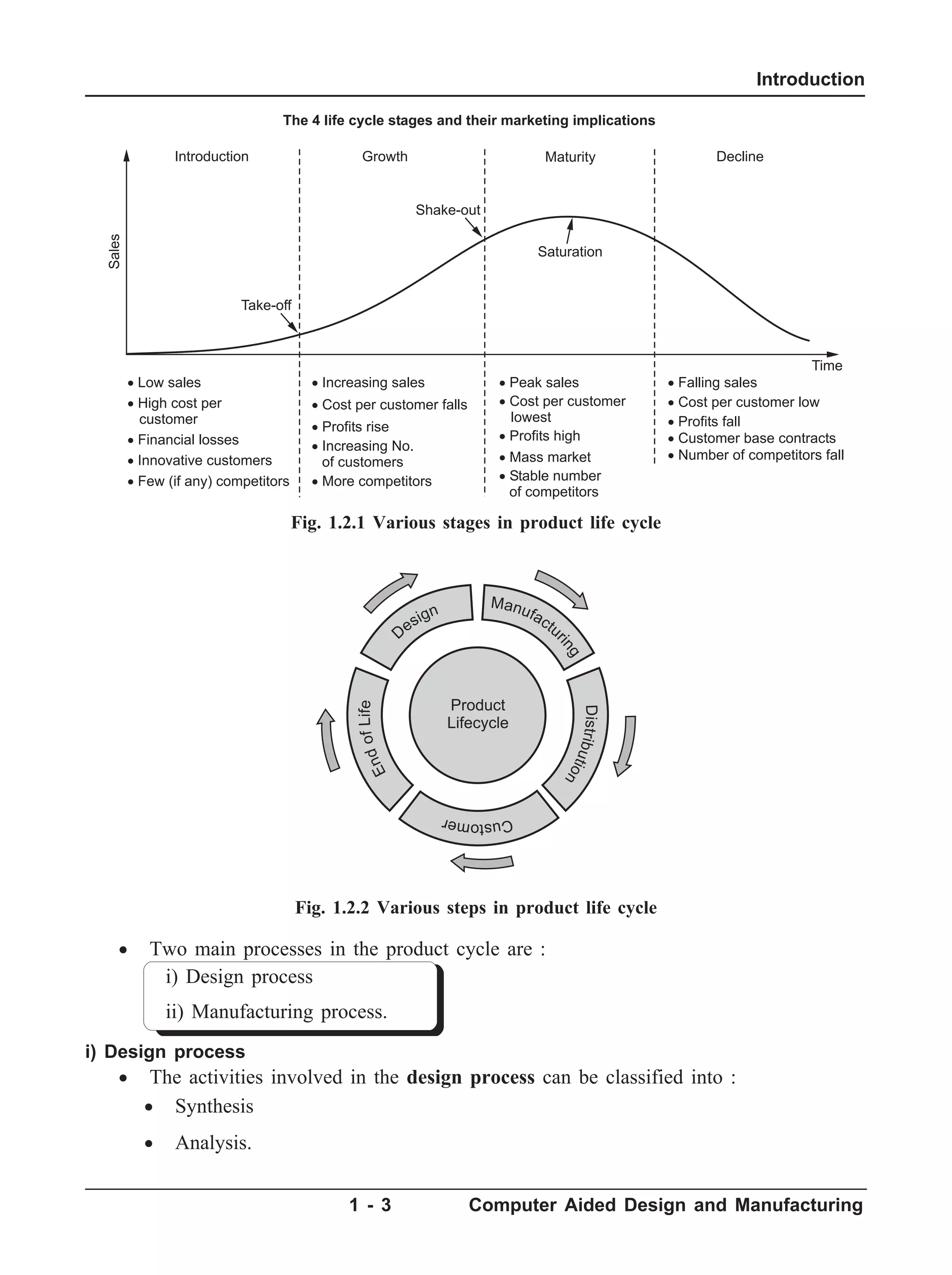
1.3 Design Process + [AU : Dec.-16]
Engineering design process :
· The engineering design process is the formulation of a plan to help an engineer
build a product with a specified performance goal. It is a decision making process
in which the basic sciences, mathematics, and engineering sciences are applied to
convert resources optimally to meet a stated objective. Fig. 1.3.1 explains
engineering design process in a detailed manner.
· The fundamental elements of the design process are the establishment of
objectives and criteria, synthesis, analysis, construction, testing and evaluation.
· The engineering design process is a multi-step process including the research,
conceptualization, feasibility assessment, establishing design requirements,
preliminary design, detailed design, production planning and tool design and
finally production.
Introduction
Design
need
Design definitions,
specifications and
requirements
Collecting relevant
design information
and feasibility study
Analysis
Design
communication
and documentation
Design
evaluation
Design
optimization
Design
analysis
Design
modeling and
simulation
Design
conceptualization
The CAD process
Synthesis
The design process
The manufacturing process
The CAM process
Process
planning
Production
planning
Design and
procurement
of new tools
Order
material
NC, CNC,
DNC
programming
Production
Quality
control
Packaging Shipping
Marketing
Fig. 1.2.3 Product cycle

Conceptual Design
It is a process in which we initiate the design and come up with a number of design
concepts and then narrow down to the single best concept. This involved the following
steps.
· Identification of customer needs : To identify the customers' needs and to
communicate them to the design team.
· Problem definition : The main goal of this activity is to create a statement that
describes what are the needs to be accomplished to meet the needs of the
customers' requirements.
· Gathering information : In this step, all the information that can be helpful for
developing and translating the customers' needs into engineering design are
collected.
· Conceptualization : In this step, broad sets of concepts are generated that can
potentially satisfy the problem statement.
· Concept selection : The main objective of this step is to evaluate the various
design concepts, modifying and evolving into a single preferred concept.
Embodiment Design
· It is a process where the structured development of the design concepts takes
place.
· It is in this phase that decisions are made on strength, material selection, size
shape and spatial compatibility.
Introduction
Define problem
Problem statement
Benchmarking
QFD
PDS
Project planning
Gather information
Internet
Patents
Trade
Literature
Concept generation
Brainstorming
Functional decomposition
Morphological chart
Evaluation of
concepts
Pugh concept selection
Decision matrix
Conceptual
design
Production architecture
Configuration design
Parametric design
Detail design
Arrangement of physical
Preliminary selection of
Robust design
Detail drawing and
specifications
elements to carry out
material and
Tolerances
functions
manfacturing
Final dimensions
modeling/sizing of parts
DFM
Embodiment
design
Fig. 1.3.1 Engineering design process

· Embodiment design is concerned with three major tasks - Product architecture,
configuration design, and parametric design.
· Product architecture : It is concerned with dividing the overall design system
into small subsystems and modules. It is in this step we decide how the physical
components of the design is to be arranged in order to combine them to carry out
the functional duties of the design.
· Configuration design: In this process we determine what all features are required
in the various parts / components and how these features are to be arranged in
space relative to each other.
· Parametric design : It starts with information from the configuration design
process and aims to establish the exact dimensions and tolerances of the product.
Also, final decisions on the material and manufacturing processes are done if it
has not been fixed in the previous process. One of the important aspects of
parametric designs is to examine if the design is robust or not.
Detail Design
· It is in this phase the design is brought to a state where it has the complete
engineering description of a tested and a producible product. Any missing
information about the arrangement, form, material, manufacturing process,
dimensions, tolerances etc. of each part is added and detailed engineering drawing
suitable for manufacturing are prepared.
Shigley's Design Process
· Fig. 1.3.2 explain the step by step procedure of Shigley's design process model.
(See Fig. 1.3.2 on next page)
· Recognition of need : The problems in the existing products (or) potential for
new products in market has to be identified.
· Definition of problem : The problem in the existing product or specification of
the new product is specified as design brief to the designers. It includes the
specification of physical and functional characteristics, cost, quality, performance
requirements etc. and requirement of design brief.
· Analysis and optimization : Each design from the synthesis stages are analysed
and optimum one is selected. It should be noted that synthesis and analysis are
highly iterative. A certain component or subsystem of the overall system
conceived by the designer in the synthesis stage is subjected to analysis. Based
on the analysis, improvements are made and redesigned. The process is repeated
until the design optimized within all the constraints imposed by designer.
· Evaluation : In this stage optimized design from the previous stage is checked
for all the specification mentioned in the design brief. A prototype of the product
is developed and experimentally checked for its performance, quality, reliability
and other aspects of product. If any discrepancies/problems are faced, it should be
fed back to the designer in the synthesis stage.
Introduction

· Presentation : After the product design passing through the evaluation stage,
drawings, diagrams, material specification, assembly lists, bill of materials etc.
which are required for product manufacturing are prepared and given to process
planning department and production department.
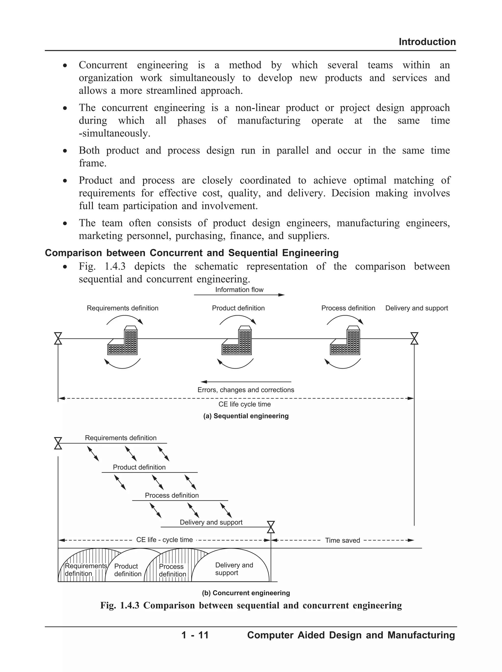
1.4 Sequential and Concurrent Engineering + [AU : May-17, Dec.-18]
Sequential Engineering (Over The Wall Engineering)
· In sequential engineering design has been carried out as a sequential set of
activities with distinct non-overlapping phases as shown in Fig. 1.4.1.
· Sequential engineering is the term used to describe the method of production in a
linear format. The different steps are done one after another, with all attention
and resources focused on that one task. After it is completed it is left alone and
everything is concentrated on the next task.
· In such an approach, the life-cycle of a product starts with the identification of
the need for that product. These needs are converted into product requirements
which are passed on to the design department.
Introduction
Recognition of need
Definition of problem
Synthesis
Analysis and optimization
Evaluation
Presentation
Success
Change the design
Can the design be improved
Design impossible for the
given specification
Fails No
Yes
Fig. 1.3.2 Shigley's design process

· The designers design the product's form, fit, and function to meet all the
requirements, and pass on the design to the manufacturing department.
· After the product is manufactured it goes through the phases of assembly, testing
and installation. This type of approach to life-cycle development is also known as
`over the wall' approach, because the different life-cycle phases are hidden or
isolated from each other.
· Each phase receives the output of the preceding phase as if the output had been
thrown over the wall. In such an approach, the manufacturing department, for
example, does not know what it will actually be manufacturing until the detailed
design of the product is over.
· There are a lot of disadvantages of the sequential engineering process. The
designers are responsible for creating a design that meets all the specified
requirements. They are usually not concerned with how the product will be
manufactured or assembled.
· Problems and inconsistencies in the designs are therefore, detected when the
product reaches into the later phases of its life-cycle.
· At this stage, the only possible option is to send the product back for a re-design.
The whole process becomes iterative and it not until after a lot of re-designs has
taken place that the product is finally manufactured.
Introduction
Design Manufacturing
· · · · · · · ·
Assembly
Fig. 1.4.1 (a) Over the wall engineering
Requirements definition Product definition Process definition Delivery and support
Errors changes and corrections
Information flow
Fig. 1.4.1 (b) Sequential engineering

Concurrent Engineering
· Due to the large number of changes, and hence iterations, the product's
introduction to market gets delayed. In addition, each re-design, re-work,
re-assembly etc. incurs cost, and therefore the resulting product is costlier than
what it was originally thought to be. The market share is lost because of the
delay in product's introduction to market, and customer faith is lost.
· Concurrent engineering is a dramatically different approach to product
development in which various life-cycle aspects are considered simultaneously
right from the early stages of design as shown in Fig. 1.4.2.
· These life-cycle aspects include product's functionality, manufacturability,
testability, assimilability, maintainability, and everything else that could be
affected by the design. In addition, various life-cycle phases overlap each other,
and there in no "wall" between these phases.
· The completion of a previous life-cycle phase is not a pre-requisite for the start
of the next life-cycle phase. In addition, there is a continuous feedback between
these life-cycle phases so that the conflicts are detected as soon as possible.
· The concurrent approach results in less number of changes during the later phases
of product life-cycle, because of the fact that the life-cycle aspects are being
considered all through the design.
· The benefits achieved are reduced lead times to market, reduced cost, higher
quality, greater customer satisfaction, increased market share etc.
· In concurrent engineering, different tasks are tackled at the same time, and not
necessarily in the usual order. This means that info found out later in the process
can be added to earlier parts, improving them, and also saving a lot of time.
Introduction
Life - cycle phases
Requirements Analysis
Detailed Design
Preliminary Design
Manufacturing
Assembly
Testing
Installation
Life Cycle Aspects (Electrical, Mechanical
Survicing, Assembiability, Recyclability, etc.)
Time
Feedback loops between
different life - cycle phases
Fig. 1.4.2 Concurrent engineering

· Concurrent engineering is a method by which several teams within an
organization work simultaneously to develop new products and services and
allows a more streamlined approach.
· The concurrent engineering is a non-linear product or project design approach
during which all phases of manufacturing operate at the same time
-simultaneously.
· Both product and process design run in parallel and occur in the same time
frame.
· Product and process are closely coordinated to achieve optimal matching of
requirements for effective cost, quality, and delivery. Decision making involves
full team participation and involvement.
· The team often consists of product design engineers, manufacturing engineers,
marketing personnel, purchasing, finance, and suppliers.
Comparison between Concurrent and Sequential Engineering
· Fig. 1.4.3 depicts the schematic representation of the comparison between
sequential and concurrent engineering.
Introduction
Requirements definition Product definition Process definition Delivery and support
Errors, changes and corrections
Information flow
Requirements definition
Product definition
Process definition
Delivery and support
CE life - cycle time Time saved
Requirements
definition
Product
definition
Process
definition
Delivery and
support
CE life cycle time
(a) Sequential engineering
(b) Concurrent engineering
Fig. 1.4.3 Comparison between sequential and concurrent engineering

Sr. No. Sequential engineering Concurrent engineering
1. Sequential engineering is the term
used to explain the method of
production in a linear system. The
various steps are done one after
another, with all attention and
resources focused on that single
task.
In concurrent engineering, various tasks
are handled at the same time, and not
essentially in the standard order. This
means that info found out later in the
course can be added to earlier parts,
improving them, and also saving time.
2. Sequential engineering is a system
by which a group within an
organization works sequentially to
create new products and services.
Concurrent engineering is a method by
which several groups within an
organization work simultaneously to create
new products and services.
3. The sequential engineering is a
linear product design process during
which all stages of manufacturing
operate in serial.
The concurrent engineering is a non-linear
product design process during which all
stages of manufacturing operate at the
same time.
4. Both process and product design
run in serial and take place in the
different time.
Both product and process design run in
parallel and take place in the same time.
5. Process and product are not
matched to attain optimal matching.
Process and product are coordinated to
attain optimal matching of requirements for
effective quality and delivery.
6. Decision making done by only
group of experts.
Decision making involves full team
involvement.
1.5 Computer Aided Design (CAD) + [AU : May-17]
The conventional design process has been accomplished on drawing boards with
design being documented in the form of a detailed engineering drawing. This process is
iterative in nature and is time consuming. The computer can be beneficially used in the
design process. The various tasks performed by a modern computer aided design system
can be grouped into four functional areas.
i) Geometric modeling
ii) Engineering analysis
iii) Design review and evaluation
iv) Automated drafting.
i) Geometric Modeling
· The geometric modeling is concerned with computer compatible mathematical
description of geometry of an object.
· The mathematical description should be such that the image of the object can be
displayed and manipulated in the computer terminal, modification on the
Introduction

geometry of the object can be done easily, it can be stored in the computer
memory, and can be retrieve back on the computer screen for review analysis or
alteration.
· Geometric modeling is classified into
a) Wireframe modeling
b) Solid modeling
c) Surface modeling
ii) Engineering Analysis
· The computer can be used to aid the analysis work such as stress-strain analysis,
heat transfer analysis, etc. The analysis can be done by using specific program
generated for it or by using general purpose software commercially available in
the market.
· The geometric models generated can be used for the analysis by properly
interfacing the modeling software with the analysis software.
· Two types of engineering analysis are
a) Analysis for mass properties
b) Finite Element Analysis (FEA)
Introduction
Recognition of need
Conventional Design Process Computer - aided design
Problem definition
Synthesis
Evaluation
Presentation
Analysis and
optimization
Geometric modeling
Engineering analysis
Design review and evaluation
Automated drafting
Fig. 1.5.1 Computer aided design process

iii) Design Review and Evaluation
· The accuracy of the design can be checked and rectified if required in the screen
itself.
· Layering feature available in software are very useful for design review purpose.
· Similarly, using the layer procedure, every stage of production can be checked.
· Suppose a new mechanism is to be designed, the same mechanism can be
simulated in the computer.
· By animation, the working of the mechanism can be checked.
· These will relieve the designer from tedious conventional method of mechanism
checking.
· Another advantage of animating the complete assembly of product is that whether
any component fouls the other components in its working.
iv) Automated Drafting
· Automated drafting is the process of creating hard copies of design drawing.
· The important features of drafting software's are automated dimensioning, scaling
of the drawing and capable of generating sectional views.
· The enlargement of minute part details and ability to generate different views of
the object like orthographic, oblique, isometric and perspective views are possible.
· Thus, CAD systems can increase productivity on drafting.
Advantages of CAD
· Efficiency, effectiveness and creativity of the designer are drastically improved.
· Faster, consistent and more accurate.
· Easy modification (copy) and improvement (edit).
· Repeating the design drawing is not needed when modifying.
· Manipulation of various dimensions, attributes is easy.
· Parametric and possess parent-child relationship.
· Inspecting tolerance and interface is easy.
· Use of standard components from part library makes fast modeling.
· Excellent graphical representation.
· Co-ordination among the groups and sharing the design data is possible.
· Exchange of e-drawing and storage of several data are easily possible.
· Graphical Simulation and animation studies the real-time behavior.
· 3D visualization of model in several orientations eliminates prototype.
· Documentation at various design phases is efficient, easier, flexible and economical.
Introduction

· Linkage to Manufacturing to carry out the production (NC/CNC programming).
· Engineering applications of CAD.
Applications of CAD :
· Structural design of Aircraft
· Aircraft simulation
· Real time simulation
· Automobile industries
· Architectural design
· Pipe routing and plan layout design
· Electronic industries
· Dynamic analysis of mechanical systems
· Kinematic analysis
· Mesh data preparation for finite element analysis.
1.6 CAD System Architecture
· In CAD, computer architecture is a set of disciplines that explains the
functionality, the organization and the introduction of computer systems; that is, it
describes the capabilities of a computer and its programming method in a
summary way, and how the internal organization of the system is designed and
executed to meet the specified facilities.
· Computer architecture engages different aspects, including instruction set
architecture design, logic design, and implementation.
· The implementation includes integrated circuit design, power, and cooling.
Optimization of the design needs expertise with compilers, operating systems and
packaging.
· Its use in designing electronic systems is known as Electronic Design
Automation, or EDA. In mechanical design it is known as Mechanical Design
Automation (MDA) or Computer-Aided Drafting (CAD), which includes the
process of creating a technical drawing with the use of computer software.
· CAD software for mechanical design uses either vector-based graphics to depict
the objects of traditional drafting, or may also produce raster graphics showing
the overall appearance of designed objects.
· However, it involves more than just shapes. As in the manual drafting of
technical and engineering drawings, the output of CAD must convey information,
such as materials, processes, dimensions, and tolerances, according to
application-specific conventions.
Introduction

· CAD may be used to design curves and figures in two-dimensional (2D) space;
or curves, surfaces, and solids in three-dimensional (3D) space.
· CAD is an important industrial art extensively used in many applications,
including automotive, shipbuilding, and aerospace industries, industrial and
architectural design, prosthetics, and many more. CAD is also widely used to
produce computer animation for special effects in movies, advertising and
technical manuals, often called DCC (Digital Content Creation).
· Fig. 1.6.1 explains CAD system architecture.
1.7 Computer Graphics
· Computer graphics involves creation, display, manipulation and storage of
pictures and experimental data for proper visualization using a computer.
· Typically, a graphics system comprises of a host computer which must have a
support of a fast processor, a large memory and frame buffer along with a few
other crucial components.
· The first of them is the display devices. Colour monitors are one example of such
display device.
· There are other examples of output devices like LCD panels, laser printers, colour
printers, plotters etc.
· Set of input devices are also needed. Typical examples are the mouse, keyboard,
joystick, touch screen, trackball etc.
Introduction
Database
(CAD model)
Application
software
Graphics
utility
Device
drivers
Input - output
devices
User
interface
System
Major classes :
Main frame
Mini computer
Workstation
Microcomputer
Based
Application areas :
Mechanical
Architectural
Construction
Circuit design
Chip design
Cost :
High end
Low end
Fig. 1.6.1 CAD system architecture

· Through these input devices it is possible to provide input to the computer and
display device is an output device which shows the image.
· The first and most important of them is the GUI as it is called. It has various
components.
· A graphical interface is basically a piece of interface or a program which exists
between the user and the graphics application program.
· It helps the graphics system to interact with the user both in terms of input and
output.
· Typical components which are used in a graphical user interface are menus,
icons, cursors, dialog boxes and scrollbars.
· Grids are used in two dimensional graphics packages to align the objects along a
set of specific coordinates or positions. It can be switched on and off and
displayed on the screen.
· Sketching is an example which is used to draw lines, arcs, poly lines and various
other objects.
· The most difficult part of the GUI is three dimensional interfaces which is
normally available at the bottom of screen.
· It is easy to interact and handle with two dimensional objects but for interacting
with the three dimensional objects three dimensional interface is needed to pick
up one of the 3D objects from a two dimensional screen.
· Essentially the computer monitor is just a two dimensional ray of pixels where
the entire picture is projected and the picture could represent a three dimensional
scene. Special facilities for 3D interface to handle or manipulate three
dimensional objects are needed.
Classification of computer graphics
· Based on the control the user has over the image
a) Passive computer graphics - The user has no control
b) Interactive graphics - The user may interact with the graphics
Introduction
Control
processor
Input
devices
Display file
Display
processor
unit
Display
screen
Link to
host computer
Control signals
Fig. 1.7.1 A basic computer graphics layout

· Based on the way the image is generated
a) Vector graphics - The image comprises of number of lines.
b) Raster graphics - Manipulation of the colour and intensity of points, pixels.
· Based on the space
a) Image-space graphics - Image itself is directly manipulated to create a picture.
b) Object-space graphics - Separate model is manipulated.
1.8 Coordinate System
Three types of coordinate systems are generally used in CAD/CAM operations as
shown in Fig. 1.8.1.
a) Model Coordinate System (MCS) or Database CS/ World CS / Master CS
b) Working Coordinate System (WCS) or User Coordinate System (UCS)
c) Screen Coordinate System (SCS) or Device CS
a) Model Coordinate System (MCS)
· It is the reference space of the model with respect to which all the model
geometrical data is stored.
· It is a Cartesian system which forms the default coordinate system used by a
particular software program.
· The X, Y, and Z axes of the MCS can be displayed on the computer screen.
· The choice of origin is arbitrary.
· The three default sketch planes of a CAD/CAM system define the three planes of
MCS, and their intersection point is the MCS origin.
Introduction
Z Z
Y Y
X X
Z'
Y'
X'
(0,0) X1
Y1
(X Y )
max' max
(a) MCS (b) WCS (c) SCS
Fig. 1.8.1

· When a CAD designer begins sketching, the origin becomes a corner point of the
profile being sketched. The sketch plane defines the orientation of the profile in
the model 3D space.
· Existing CAD/CAM software uses the MCS as the default WCS.
· The MCS is the only coordinate system that the software recognizes when storing
or retrieving graphical information from a model database. Many existing
software package allow the user to input Cartesian and cylindrical coordinates.
This input information is transformed to (x, y, z) coordinates relative to the MCS
before being stored in the database.
b) Working Coordinate System (WCS) or User Coordinate System (UCS)
· This is basically an auxiliary coordinate system used in place of MCS. For
convenience while we develop the geometry by data input this kind of coordinate
system is useful.
· It is very useful when a plane (face) in MCS is not aligned (easily defined) along
any orthogonal planes.
· It can be established at any position and orientation in space that the user desires.
· The user can define a Cartesian coordinate system whose XY plane is coincident
with the desired plane of construction. That new system is called as WCS.
· It is a user defined system that facilitates the geometrical construction. While user
inputs data in WCS the software transforms it to MCS before storing the data.
· There is only one active WCS at any one time. If the user defines multiple
WCSs in one session, the software recognizes only the last one.
c) Screen Coordinate System (SCS)
· In contrast to MCS and WCS, Screen Coordinate System is a two-dimensional
device-independent system whose origin is usually located at the lower left corner
of the graphic display (display screen).
· The physical dimensions of the device screen and the type of device determine
the range of the SCS. A 1024 ´ 1024 display has an SCS with a range of (0, 0)
to (1024,1024).
· The SCS is important for display, screen input and digitizing tasks.
· A transformation operation from MCS coordinates to SCS coordinates is
performed by the software before displaying the model views and graphics.
· For a geometric model, there is a data structure to store its geometric data
(relative to MCS), and a display file to store its display data (relative to SCS).
Window and View Port
Window
· When a design package is initiated, the display will have a set of co-ordinate
values. These are called default co-ordinates.
Introduction

· A user co-ordinate system is one in which the designer can specify his own
coordinates for a specific design application.
· These screen independent coordinates can have large or small numeric range, or
even negative values, so that the model can be represented in a natural way.
· It may, however, happen that the picture is too crowded with several features to
be viewed clearly on the display screen.
· Therefore, the designer may want to view only a portion of the image, enclosed
in a rectangular region called a window.
· Different parts of the drawing can thus be selected for viewing by placing the
windows.
· Portions inside the window can be enlarged, reduced or edited depending upon
the requirements. Fig. 1.8.2 (a) depicts the use of windowing to enlarge an image.
View Port
· It may be sometimes desirable to display different portions or views of the
drawing in different regions of the screen.
· A portion of the screen where the contents of the window are displayed is called
a view port. Fig. 1.8.2 (b) explains a view port.
1.9 2D Transformations + [AU : Dec.-17]
· Geometric transformations provide a means by which an image can be enlarged
in size, or reduced, rotated, or moved.
· These changes are brought about by changing the co-ordinates of the picture to a
new set of values depending upon the requirements.
· The basic transformations are translation, scaling, rotation, reflection or mirror
and shear.
Introduction
Window
Original
drawing
65,50
130,100 View port 1
View port 4 View port 3
View port 2
(a) Window (b) View port
Fig. 1.8.2

a) 2D Translation
· This moves a geometric entity in space in such a way that the new entity is
parallel at all points to the old entity. Translation of a point is shown in
Fig. 1.9.1.
· Let's consider a point on the object, represented by P which is translated along X
and Y axes by DX and DY respectively to a new position P '.
· The new coordinates after transformation are given by following equations.
P' = [x', y' ] …(1.9.1)
x' = [x+Dx] …(1.9.2)
y' = [y+Dy] …(1.9.3)
[P'] =
¢
¢
é
ë
ê
ù
û
ú
x
y
=
x x
y y
+
+
é
ë
ê
ù
û
ú
D
D
=
x
y
é
ë
ê
ù
û
ú +
D
D
x
y
é
ë
ê
ù
û
ú …(1.9.4)
2D Translation of an object
Fig. 1.9.2 explains the transformation of a rectangle. Consider a rectangle of
coordinates (1,1), (4,1), (1,5) and (4,5). The rectangle is translated by 3 units along
x-direction (Dx) and 3 units along y-direction (Dy). (See Fig. 1.9.2 on next page)
b) 2D Scaling
· Scaling is the transformation applied to change the scale of an entity.
· To achieve scaling, the original coordinates would be multiplied uniformly by the
scaling factors.
Sx = Scaling factor along x-direction
Sy = Scaling factor along y-direction
Ts = Scaling matrix
· The scaling operations could be explained by the equations stated below.
¢
P = [x', y' ]=[Sx ´ X, Sy ´ Y] …(1.9.5)
Introduction
P
P Z
Y
X
X
P'
X'
Y'
Z'
Y
Fig. 1.9.1 Translation of a point

[ ¢
P ] =
S 0
0 S
x
y
x
y
é
ë
ê
ù
û
ú
é
ë
ê
ù
û
ú …(1.9.6)
[Ts] =
S 0
0 S
x
y
é
ë
ê
ù
û
ú …(1.9.7)
[ ¢
P ] = [Ts] × [P] …(1.9.8)
· Fig. 1.9.3 depicts the scaling of an
object.
c) 2D Rotation
· Rotation is another important
geometric transformation. The
final position and orientation of a
geometric entity is decided by the
angle of rotation (q) and the base
point about which the rotation, is
to be done.
· If rotation is made in clockwise
direction 'q' is considered as
Introduction
0 1 2 3 4 5 6 7 8 9 10
X
(1, 1) (4, 1)
(1, 5) (4, 5)
(5, 4) (8, 4)
(5, 8) (8, 8)
Y
0
1
2
3
4
5
6
7
8
9
10
Original rectangle
After translation
Fig. 1.9.2 2D Translation of an object
X
SX
SY
Y
P
P'
Y
X
Fig. 1.9.3 2D Scaling of an object

negative and if rotation is made in counter clockwise (anti-clockwise) direction
' q' is considered as positive.
· Fig. 1.9.4 depicts rotation of an object.
· To develop the transformation matrix for transformation, consider a point P
located in XY-plane, being rotated in the counter clockwise direction to the new
position, ¢
P by an angle 'q' as shown in Fig. 1.9.4. The new position ¢
P is given
by
¢
P = [ ¢
x , ¢
y ]
· From the figure the original position is specified by
x = r cos a
y = r sin a
· The new position ¢
P is specified by
¢
x = r cos ( +
a q) = r cos q cos a – r sin q sin a
= x cos q – y sin q
Also, ¢
y = r sin ( +
a q) = r sin q cos a + r cos q sin a
= x sin q + y cos q
· Thus the transformation matrix for a rotation operation could be derived as
follows,
[P ]
¢ =
¢
¢
é
ë
ê
ù
û
ú
x
y
=
cos sin
sin cos
x
y
q q
q q
-
é
ë
ê
ù
û
ú
é
ë
ê
ù
û
ú …(1.9.9)
· The rotation matrix is given as TR .
Introduction
X'
X
P'
r
P
X
Y
Y'
Y
0
Fig. 1.9.4 2D rotation of an objects

[TR ] =
cos sin
sin cos
q q
q q
-
é
ë
ê
ù
û
ú …(1.9.10)
[P ]
¢ = [T [P]
R ]× (1.9.11)
d) 2D Shearing
· A shearing transformation produces distortion of an object or an entire image.
There are two types of shears : X-shear and Y-shear.
· A transformation that slants the shape of an object is called the shear
transformation.
· One shifts X coordinates values and other shifts Y coordinate values. However;
in both the cases only one coordinate changes its coordinates and other preserves
its values.
· Shearing is also termed as skewing.
· The X-shear as shown in the Fig. 1.9.5 (a), preserves the Y coordinate and
changes are made to X coordinates, which causes the vertical lines to tilt right or
left.
Introduction
11 12 13
After X-shear
Original part
D1
A1
B1
A B
E1
C1
C
D
0 1 2 3 4 5 6 7 8 9 10
X
Y
0
1
2
3
4
5
6
7
8
9
10
E
Fig. 1.9.5 (a) X-Shear

· The Y-shear as shown in the Fig. 1.9.5 (b) preserves the X coordinates and
changes the Y coordinates which causes the horizontal lines to transform into
lines which slopes up or down.
· A Y-shear transforms the point (x, y) to the point (x1, y1) by a factor Sh1,
¢
x = x …(1.9.12)
¢
y = Sh x y
1 × + …(1.9.13)
· An X-shear transforms the point (X, Y) to (x1, y1), where Sh2 is the shear factor
¢
x = x + Sh y
2 × …(1.9.14)
¢
y = y …(1.9.15)
e) 2D Reflection/Mirror
· Reflection is the mirror image of original object.
· Mirroring is a convenient method used for copying an object while preserving its
features.
· In reflection transformation, the size of the object does not change.
· Reflection could be done along both x and y directions as shown in the
Fig.1.9.6(a) and 1.9.6(b).
Introduction
After X-shear
Original part
D1
C1
B1
E1
0 1 2 3 4 5 6 7 8 9 10
X
Y
0
1
2
3
4
5
6
7
8
9
10
E
D
C
B
A
A1
Fig. 1.9.5 (b) Y-Shear

· For reflection about x-axis the y coordinate will be negative and the following
equations should be utilized,
¢
P = [X , Y ]
¢ ¢ = [X, – Y] …(1.9.16)
[P ]
¢ =
1 0
0 1
-
é
ë
ê
ù
û
ú
é
ë
ê
ù
û
ú
x
y
…(1.9.17)
The translation matrix is given as,
[T ]
m =
1 0
0 1
-
é
ë
ê
ù
û
ú …(1.9.18)
[P ]
¢ = [T ] [P]
m × …(1.9.19)
· For reflection about y-axis the x coordinate will be negative and the following
equations should be utilized,
¢
P = [X , Y ]
¢ ¢ = [X, – Y] …(1.9.20)
[P ]
¢ =
-
é
ë
ê
ù
û
ú
é
ë
ê
ù
û
ú
1 0
0 1
x
y
…(1.9.21)
The translation matrix is given as,
[T ]
m =
-
é
ë
ê
ù
û
ú
1 0
0 1
…(1.9.22)
[P ]
¢ = [T ] [P]
m × …(1.9.23)
· Thus the general form of reflection matrix could be written as,
[T ]
m =
±
±
é
ë
ê
ù
û
ú
1 0
0 1
…(1.9.24)
Introduction
(a) Reflection about X-Axis
P
Y
X
Y
–
Y
P'
– X X
Y
X
P
P'
(b) Reflection about Y-axis
Fig. 1.9.6

1.9.1 Homogeneous Coordinates
Concatenation of Transformations
· Sometimes it becomes necessary to combine the individual transformations in
order to achieve the required results. In such cases the combined transformation
matrix can be obtained by multiplying the respective transformation matrices as
shown below,
[P ]
¢ = [T ][T ][T ]...[T ][T ][T ]
n n 1 n 2 3 2 1
- - …(1.9.25)
· In order to concatenate the transformation, all the transformation matrices should
be multiplicative type. The following form known as homogeneous form should
be used to convert the translation matrix into a multiplication type.
[P ]
¢ =
¢
¢
é
ë
ê
ê
ê
ù
û
ú
ú
ú
x
y
1
=
1 0 0
0 1 0
D D
X Y 1
x
y
1
é
ë
ê
ê
ê
ù
û
ú
ú
ú
é
ë
ê
ê
ê
ù
û
ú
ú
ú
…(1.9.26)
· The three dimensional representation of a two dimensional plane is called
homogeneous coordinates and the transformation using the homogeneous
co-ordinates is called homogeneous transformation.
· The translation matrix in homogeneous form is,
[T] =
1 0 0
0 1 0
D D
X Y 1
é
ë
ê
ê
ê
ù
û
ú
ú
ú
· The Scaling matrix in homogeneous form is,
[S] =
S 0 0
0 S 0
0 0 1
x
y
é
ë
ê
ê
ê
ù
û
ú
ú
ú
· The Rotation matrix in homogeneous form is,
[T ]
R =
cos sin
sin cos
q q
q q
0
0
0 0 1
-
é
ë
ê
ê
ê
ù
û
ú
ú
ú
Need for homogeneous transformation
· Consider the need for rotating an object about an arbitrary point as shown in
Fig. 1.9.7.
· The transformation given earlier for rotation is about the origin of the axes
system.
· To derive the necessary transformation matrix, the following complex procedure
would be required.
i) Translate the point 'P' to 'O', the origin of the axes system.
Introduction

ii) Rotate the object by the given angle 'q'.
iii) Translate the point back to its original position from origin.
· The following homogeneous transformation matrices should be used for the
translation operation,
i) Translate the point from point 'P' to origin 'O'
[T ]
1 = [T] =
1 0 0
0 1 0
1
- -
é
ë
ê
ê
ê
ù
û
ú
ú
ú
D D
X Y
ii) Rotate the object by the given angle 'q'.
[T ]
2 = [T ]
R =
cos sin
sin cos
q q
q q
0
0
0 0 1
-
é
ë
ê
ê
ê
ù
û
ú
ú
ú
iii) Translate the point back to its original position from origin.
[T ]
3 = [T] =
1 0 0
0 1 0
1
D D
X Y
é
ë
ê
ê
ê
ù
û
ú
ú
ú
iv) Final Transformation matrix after concatenation,
[T] = [T ] [T ] [T ]
1 2 3
´ ´
Introduction
A
X
Y
r
r
P'
P
O
Y
X
Fig. 1.9.7 Rotation of an object about an arbitrary point

1.9.2 Solved Examples on 2D Transformation
Example 1.9.1 : Translate a point P(2, 3) by four units in x-direction and 5 units in
y-direction.
Solution : Given : P(2, 3) Þ (x , y )
1 1
Dx = 4; Dy = 5
Tranformation matrix
T =
D
D
x
y
é
ë
ê
ù
û
ú
New position of a point is,
¢
P = P + T
¢
¢
é
ë
ê
ù
û
ú
x
y
1
1
=
x
y
x
y
1
1
é
ë
ê
ù
û
ú +
é
ë
ê
ù
û
ú
D
D
=
2
3
4
5
é
ë
ê
ù
û
ú +
é
ë
ê
ù
û
ú =
6
8
é
ë
ê
ù
û
ú
Example 1.9.2 : A line AB, A(2, 4) and B(5, 6) is to be translated 1 unit along +ve
direction of 'x' and 3 units along +ve direction of y. Find the translated coordinates.
Solution : Given :
For line AB ® A(x , y )
1 1 = (2, 4)
B(x , y )
2 2 = (5, 6)
T x y
(D , D ) = (1, 3)
Introduction
y = 5
P
(2, 3)
P'(6, 8)
X
Y
x = 4
Fig. 1.9.8

¢
A = A + T
¢
A =
2
4
1
3
é
ë
ê
ù
û
ú +
é
ë
ê
ù
û
ú =
3
7
é
ë
ê
ù
û
ú
Similarly ¢
B = B + T =
5
6
1
3
é
ë
ê
ù
û
ú +
é
ë
ê
ù
û
ú =
6
9
é
ë
ê
ù
û
ú
Example 1.9.3 : Translate a triangle ABC having coordinates A(1, 1), B(3, 1) and
C(1, 3) about the origin by 3 - units in x - direction and 2 - units in y - direction.
Solution : Given : Triangle ABC,
A = (x , y )
1 1 = (1, 1)
B = (x , y )
2 2 = (3, 1)
C = (x , y )
3 3 = (1, 3)
Dx = 3; Dy = 2 Þ T = (3, 2)
¢
A = A + T =
1
1
3
2
é
ë
ê
ù
û
ú +
é
ë
ê
ù
û
ú =
4
3
é
ë
ê
ù
û
ú
Introduction
x = 1
A
(2, 4)
B (5, 6)
B' (6, 9)
A' (3, 7)
X
Y
y = 3
Fig. 1.9.9

¢
B = B + T =
3
1
3
2
é
ë
ê
ù
û
ú +
é
ë
ê
ù
û
ú =
6
3
é
ë
ê
ù
û
ú
¢
C = C + T =
1
3
3
2
é
ë
ê
ù
û
ú +
é
ë
ê
ù
û
ú =
4
5
é
ë
ê
ù
û
ú
Example 1.9.4 : A rectangular lamina ABCD having co-ordinates A(2, 2), B(4, 2),
C(4, 5) and D(2, 5) is translated by 4 units in x - direction and 4 units in y - direction.
Find out the translated coordinates and plot the rectangle before and after translation.
Solution : Given : Rectangle ABCD,
A (2, 2) = (x , y )
1 1
B (4, 2) = (x , y )
2 2
C (4, 5) = (x , y )
3 3
D (2, 5) = (x , y )
4 4
Dx = 4; Dy = 4 Þ T( , )
D D
x y = (4, 4)
[A] = [A] + [T] =
2
2
4
4
é
ë
ê
ù
û
ú +
é
ë
ê
ù
û
ú =
6
6
é
ë
ê
ù
û
ú
[B ]
¢ = [B] + [T] =
4
2
4
4
é
ë
ê
ù
û
ú +
é
ë
ê
ù
û
ú =
8
6
é
ë
ê
ù
û
ú
Introduction
x = 3
y = 2
C (1, 3)
A' (4, 3)
B (3, 1)
A (1, 1)
B' (6, 3)
C' (4, 5)
X
Y
Fig. 1.9.10

[C ]
¢ = [C] + [T] =
4
5
4
4
é
ë
ê
ù
û
ú +
é
ë
ê
ù
û
ú =
8
9
é
ë
ê
ù
û
ú
[D ]
¢ = [D] + [T] =
2
5
4
4
é
ë
ê
ù
û
ú +
é
ë
ê
ù
û
ú =
6
9
é
ë
ê
ù
û
ú
Example 1.9.5 : A polygon ABCD is having the coordinates A(2, 3), B(6, 3), C(6, 6),
D(2, 6). Scale the polygon by 2 units along x-axis and y-axis.
Solution : Given :
Polygon ABCD ® A(x , y )
1 1 = (2, 3)
B(x , y )
2 2 = (6, 3)
C(x , y )
3 3 = (6, 6)
D(x , y )
4 4 = (2, 6)
Scaling factor ® S = (S ,S )
x y = (2, 2)
Scaling matrix, [S] =
S 0
0 S
x
y
é
ë
ê
ù
û
ú =
2 0
0 2
é
ë
ê
ù
û
ú
Introduction
(6, 9)
(6, 6)
C' (8, 9)
x = 4
(2, 5)
(2, 2)
C (4, 5)
B (4, 2)
A
D
(8, 6)
B'
D'
y = 4
A'
X
Y
Fig. 1.9.11

[A]¢ = [S] ´ [A]
=
2 0
0 2
2
3
é
ë
ê
ù
û
ú ´
é
ë
ê
ù
û
ú =
4
6
é
ë
ê
ù
û
ú
[B]¢ = [S] ´ [B] Þ
=
2 0
0 2
6
3
é
ë
ê
ù
û
ú ´
é
ë
ê
ù
û
ú =
12
6
é
ë
ê
ù
û
ú
[C]¢ = [S] ´ [C]
=
2 0
0 2
6
6
é
ë
ê
ù
û
ú ´
é
ë
ê
ù
û
ú =
12
12
é
ë
ê
ù
û
ú
[D]¢ = [S] ´ [D]
=
2 0
0 2
2
6
é
ë
ê
ù
û
ú ´
é
ë
ê
ù
û
ú =
4
12
é
ë
ê
ù
û
ú
Introduction
X
Y
A (2, 3)
D (2, 6)
A' (4, 6)
C (6, 6)
B' (12, 6)
C' (12, 12)
D' (4, 12)
B (6, 3)
Fig. 1.9.12

Example 1.9.6 : Rotate the point P(6, 8) about the origin at an angle 30 ° in
anti-clock wise direction and obtain the new position of the point.
Solution : Given
P(x , y )
1 1 = (6, 8) ; q = 30°
¢
P =
¢
¢
é
ë
ê
ù
û
ú
x
y
1
1
=
cos sin
sin cos
q q
q q
-
é
ë
ê
ù
û
ú
é
ë
ê
ù
û
ú
x
y
1
1
=
cos sin
sin cos
30 30
30 30
-
é
ë
ê
ù
û
ú
é
ë
ê
ù
û
ú
6
8
Þ [P ]
¢ =
1.196
9.928
é
ë
ê
ù
û
ú
Example 1.9.7 : A triangle ABC, A(5, 2), B(3, 5), C(7, 5). Find the transformed
position if,
i) The triangle is rotated by 45 ° in clockwise direction.
ii) The triangle is rotated by 60 ° in anti-clockwise direction.
Solution : Given : DABC Þ A(5, 2)
(x , y )
,
B(3, 5)
(x , y )
,
C(7, 5)
(x , y )
1 1 2 2 3 3
i) Rotated by 45 ° in clockwise direction :
q = – 45°
[A]¢ =
¢
¢
é
ë
ê
ù
û
ú
x
y
1
1
=
cos( ) sin( )
sin( ) cos( )
- ° - - °
- ° - °
é
ë
ê
ù
û
ú
é
ë
ê
ù
û
45 45
45 45
5
2ú
Introduction
Y
X
30° =
P' (1.196, 9.28)
P(6, 8)
Fig. 1.9.13

Þ [A]¢ =
4.97
2.12
-
é
ë
ê
ù
û
ú
Similarly, [B]¢ =
¢
¢
é
ë
ê
ù
û
ú
x
y
2
2
=
cos( ) sin( )
sin( ) cos( )
- ° - - °
- ° - °
é
ë
ê
ù
û
ú
é
ë
ê
ù
û
45 45
45 45
3
5ú
Þ [B]¢ =
5.65
1.41
é
ë
ê
ù
û
ú
Similarly, [C]¢ =
¢
¢
é
ë
ê
ù
û
ú
x
y
3
3
=
cos( ) sin( )
sin( ) cos( )
- ° - - °
- ° - °
é
ë
ê
ù
û
ú
é
ë
ê
ù
û
45 45
45 45
7
5ú
Þ [C]¢ =
8.48
1.414
-
é
ë
ê
ù
û
ú
ii) Rotated by 60° in anticlockwise direction (counter-clockwise) :
q = 60°
[A]¢¢ =
¢¢
¢¢
é
ë
ê
ù
û
ú
x
y
1
1
=
cos sin
sin cos
60 60
60 60
5
2
-
é
ë
ê
ù
û
ú
é
ë
ê
ù
û
ú
Þ [A]¢¢ =
0.767
5.330
é
ë
ê
ù
û
ú
Similarly, [B]¢¢ =
¢¢
¢¢
é
ë
ê
ù
û
ú
x
y
2
2
=
cos sin
sin cos
60 60
60 60
3
5
-
é
ë
ê
ù
û
ú
é
ë
ê
ù
û
ú
Þ [B]¢¢ =
-
é
ë
ê
ù
û
ú
2.830
5.098
Similarly, [C]¢¢ =
¢¢
¢¢
é
ë
ê
ù
û
ú
x
y
3
3
=
cos sin
sin cos
60 60
60 60
7
5
-
é
ë
ê
ù
û
ú
é
ë
ê
ù
û
ú
Þ [C]¢¢ =
-
é
ë
ê
ù
û
ú
0.83
8.562
Introduction

Example 1.9.8 : A square with an edge length of 10 units is located in the origin with
one of the edges inclined at an angle 30 ° with X-axis. Calculate the new position of the
square, i) If it is rotated by an angle 30 ° in clock-wise direction. ii) If it is rotated by
60° in counter-clockwise direction.
Solution : Given : Square of edge
length 10 units.
® Positioned in such a way that, it
is located in origin ® with one of the
edges inclined by 30 ° to 'X'
(Refer Fig.1.9.15).
Initially evaluate the coordinates of
the square.
Þ A(x , y )
1 1 = (0, 0). Since place
at the origin.
Þ B(x , y )
2 2
Introduction
0
A" (0.767, 5.330)
(–0.830, 8.582)
(–2.830, 5.098)
60°
45°
B(3, 5)
C(7, 5)
A(5, 2)
A' (4.97, –2.12)
C' (8.48, –1.41)
B' (5.65, 1.41)
X
Y
Y
X
B"
C"
Fig. 1.9.14
60° 30°
(x , y )
3 3
(x , y )
1 1
(x , y )
2 2
D
B
C
Y
X X
A (0, 0)
0
Fig. 1.9.15

B(x , y )
2 2 :
Here edge length = 10 units
x2 = 10 cos 30 = 8.66 units
y 2 = 10 sin 30 = 5 units
B(x , y )
2 2 = (8.66, 5)
Similarly, C(x , y )
3 3 :
x 3 = x2 -10 60
cos
= 8.66 – 5 = 3.66 units
y 3 = y 2 +10 60
sin
= 5 + 8.66 = 13.66 units
C(x , y )
3 3 = (3.66, 13.66)
[D](x , y )
4 4 :
x4 = – 10 cos 60
= – 5 units
Introduction
Y
A (0, 0)
X
y2
x2
l = 10
30°
(x , y )
2 2
B
Fig. 1.9.16
Y
A (0, 0)
X
y2
x2
(x , y )
2 2
(x , y )
3 3
10 sin 60
B
60°
30°
30°
l = 10
10 cos 60
Fig. 1.9.17
Y
X
l=10 10 sin 60
– 10 cos 60
D(x , y )
4 4
60°
Fig. 1.9.18

y 4 = 10 sin 60 = 8.66 units
D(x , y )
4 4 = (– 5, 8.66)
i) Rotate the square by 30° clockwise :
q = – 30°
[A]¢ =
cos( ) sin( )
sin( ) cos( )
- - -
- -
é
ë
ê
ù
û
ú
é
ë
ê
ù
û
ú
30 30
30 30
0
0
=
0
0
é
ë
ê
ù
û
ú
[B]¢ =
cos( ) sin( )
sin( ) cos( )
- - -
- -
é
ë
ê
ù
û
ú
é
ë
ê
ù
û
ú
30 30
30 30 5
8.66
=
9.99 ~ 10
0.0001~ 0
é
ë
ê
ù
û
ú
Þ [B]¢ =
10
0
é
ë
ê
ù
û
ú
[C]¢ =
cos( ) sin( )
sin( ) cos( )
- - -
- -
é
ë
ê
ù
û
ú
é
ë
30 30
30 30
3.66
13.66
ê
ù
û
ú =
10
10
é
ë
ê
ù
û
ú
[D]¢ =
cos( ) sin( )
sin( ) cos( )
- - -
- -
é
ë
ê
ù
û
ú
-
é
ë
ê
ù
û
30 30
30 30
5
8.66ú =
0
10
é
ë
ê
ù
û
ú
iii) Square is rotated by 60° in counter clockwise direction :
q = 60°
[A]¢¢ =
cos sin
sin cos
60 60
60 60
0
0
-
é
ë
ê
ù
û
ú
é
ë
ê
ù
û
ú =
0
0
é
ë
ê
ù
û
ú
[B]¢¢ =
cos sin
sin cos
60 60
60 60
-
é
ë
ê
ù
û
ú
é
ë
ê
ù
û
ú
8.66
5
=
0
10
é
ë
ê
ù
û
ú
[C]¢¢ =
cos sin
sin cos
60 60
60 60
-
é
ë
ê
ù
û
ú
é
ë
ê
ù
û
ú
3.66
13.66
=
-
é
ë
ê
ù
û
ú
10
10
[D]¢¢ =
cos sin
sin cos
60 60
60 60
5
-
é
ë
ê
ù
û
ú
-
é
ë
ê
ù
û
ú
8.66
=
-
é
ë
ê
ù
û
ú
10
0
Introduction

Example 1.9.9 : For a planar lamina ABCD with A(3, 5), B(2, 2), C(8, 2) and D(4, 5)
in XY plane with point P(4, 3) in the inetrior is to be
i) Translated by a translation matrix [T] =
8
5
é
ë
ê
ù
û
ú
ii) Rotated by 60° in counter clockwise direction.
Introduction
60° 30°
D''
(–10, 0)
B' (10, 0)
C' (10, 10)
C
(3.66, 13.66)
C"
(–10, 10) D' B''
(0, 10)
B
A (0, 0)
A', A"
Fig. 1.9.19
A (3, 5) D(4, 5)
P
(4, 3)
B (2, 2) C (8, 2)
Fig. 1.9.20

Sol. : i) Translation :
[T] =
D
D
x
y
é
ë
ê
ù
û
ú =
8
5
é
ë
ê
ù
û
ú
Dx = 8; Dy = 5
[A]¢ =
x
y
x
y
1
1
é
ë
ê
ù
û
ú +
é
ë
ê
ù
û
ú
D
D
=
3
5
8
5
é
ë
ê
ù
û
ú +
é
ë
ê
ù
û
ú =
11
10
é
ë
ê
ù
û
ú
[B]¢ =
x
y
x
y
2
2
é
ë
ê
ù
û
ú +
é
ë
ê
ù
û
ú
D
D
=
2
2
8
5
é
ë
ê
ù
û
ú +
é
ë
ê
ù
û
ú =
10
7
é
ë
ê
ù
û
ú
[C]¢ =
x
y
x
y
3
3
é
ë
ê
ù
û
ú +
é
ë
ê
ù
û
ú
D
D
=
8
2
8
5
é
ë
ê
ù
û
ú +
é
ë
ê
ù
û
ú =
16
7
é
ë
ê
ù
û
ú
[D]¢ =
x
y
x
y
4
4
é
ë
ê
ù
û
ú +
é
ë
ê
ù
û
ú
D
D
=
4
5
8
5
é
ë
ê
ù
û
ú +
é
ë
ê
ù
û
ú =
12
10
é
ë
ê
ù
û
ú
[P]¢ =
4
3
x
y
é
ë
ê
ù
û
ú +
é
ë
ê
ù
û
ú
D
D
=
4
3
8
5
é
ë
ê
ù
û
ú +
é
ë
ê
ù
û
ú =
12
8
é
ë
ê
ù
û
ú
ii) Rotate through 60° in counter clockwise direction :
q = 60°
[A]¢¢ =
cos sin
sin cos
60 60
60 60
3
5
-
é
ë
ê
ù
û
ú
é
ë
ê
ù
û
ú =
-
é
ë
ê
ù
û
ú
2.83
5.09
[B]¢¢ =
cos sin
sin cos
60 60
60 60
-
é
ë
ê
ù
û
ú
é
ë
ê
ù
û
ú
2
2
=
-
é
ë
ê
ù
û
ú
0.732
2.732
[C]¢¢ =
cos sin
sin cos
60 60
60 60
-
é
ë
ê
ù
û
ú
é
ë
ê
ù
û
ú
8
2
=
2.26
7.93
é
ë
ê
ù
û
ú
[D]¢¢ =
cos sin
sin cos
60 60
60 60
4
-
é
ë
ê
ù
û
ú
é
ë
ê
ù
û
ú
5
=
-
é
ë
ê
ù
û
ú
2.33
5.96
[P]¢¢ =
cos sin
sin cos
60 60
60 60
4
-
é
ë
ê
ù
û
ú
é
ë
ê
ù
û
ú
3
=
-
é
ë
ê
ù
û
ú
0.59
4.96
Introduction

Introduction
1
2
3
4
5
6
7
8
9
10
11
12
13
14
Y
–3
–2
–1
0
1
2
3
4
5
6
7
8
9
10
11
12
13
14
15
16
D''
A''
C''
A
D
B
C
B'
A'
D'
C'
P'
X
X
Y
P"
B"
P
Fig. 1.9.21

Example 1.9.10 : Derive an appropriate 2D transformation method to reflect the
rectangle ABCD, A(3, 4), B(7, 4), C(7, 6), D(3, 6). Reflect about i) X-axis, ii) Y-axis.
Solution : i) For reflection about X-axis :
[A]¢ =
1 0
0 1
-
é
ë
ê
ù
û
ú
é
ë
ê
ù
û
ú
x
y
1
1
Þ [A]¢ =
1 0
0 1
-
é
ë
ê
ù
û
ú
é
ë
ê
ù
û
ú
3
4
=
3
4
-
é
ë
ê
ù
û
ú
[B]¢ =
1 0
0 1
-
é
ë
ê
ù
û
ú
é
ë
ê
ù
û
ú
7
4
=
7
4
-
é
ë
ê
ù
û
ú
[C]¢ =
1 0
0 1
-
é
ë
ê
ù
û
ú
é
ë
ê
ù
û
ú
7
6
=
7
6
-
é
ë
ê
ù
û
ú
[D]¢ =
1 0
0 1
-
é
ë
ê
ù
û
ú
é
ë
ê
ù
û
ú
3
6
=
3
6
-
é
ë
ê
ù
û
ú
Introduction
A
(3, 4)
B
D' C'
(7, 4)
(3, – 6) (7, – 6)
D
(3, 6)
C
(7, 6)
A'
(3, – 4) B'(7, – 4)
X
Y
Y
X
Fig. 1.9.22

ii) Reflection about Y-axis :
[A]¢ =
-
é
ë
ê
ù
û
ú
é
ë
ê
ù
û
ú
1 0
0 1
x
y
1
1
Þ [A]¢ =
-
é
ë
ê
ù
û
ú
é
ë
ê
ù
û
ú
1 0
0 1
3
4
=
-
é
ë
ê
ù
û
ú
3
4
[B]¢ =
-
é
ë
ê
ù
û
ú
é
ë
ê
ù
û
ú
1 0
0 1
7
4
=
-
é
ë
ê
ù
û
ú
7
4
[C]¢ =
-
é
ë
ê
ù
û
ú
é
ë
ê
ù
û
ú
1 0
0 1
7
6
=
-
é
ë
ê
ù
û
ú
7
6
[D]¢ =
-
é
ë
ê
ù
û
ú
é
ë
ê
ù
û
ú
1 0
0 1
3
6
=
-
é
ë
ê
ù
û
ú
3
6
iii) About origin :
[A]¢¢¢ =
-
-
é
ë
ê
ù
û
ú
é
ë
ê
ù
û
ú
1 0
0 1
x
y
1
1
Introduction
(–7, 6)
D''(–3, 6) D(3, 6)
A''(–3, 4)
(–7, 4)
A(3, 4) B(7, 4)
C(7, 6)
X
Y
Y
X
C''
B''
Fig. 1.9.23

Þ [A]¢¢¢ =
-
-
é
ë
ê
ù
û
ú
é
ë
ê
ù
û
ú
1 0
0 1
3
4
=
-
-
é
ë
ê
ù
û
ú
3
4
[B]¢¢¢ =
-
-
é
ë
ê
ù
û
ú
é
ë
ê
ù
û
ú
1 0
0 1
7
4
=
-
-
é
ë
ê
ù
û
ú
7
4
[C]¢¢¢ =
-
-
é
ë
ê
ù
û
ú
é
ë
ê
ù
û
ú
1 0
0 1
7
6
=
-
-
é
ë
ê
ù
û
ú
7
6
[D]¢¢¢ =
-
-
é
ë
ê
ù
û
ú
é
ë
ê
ù
û
ú
1 0
0 1
3
6
=
-
-
é
ë
ê
ù
û
ú
3
6
2-D Transformation Problems based on Homogeneous Coordinate System
(Concatenation)
Example 1.9.11 : A rectangle ABCD has coordinates A(2, 3), B(6, 3), C(6, 6) and
D(2, 6). Calculate the combined transformation matrix (concatenation) for the following
operations. Also find the resultant coordinates.
i) Translation by 2 units in x - direction and 3 units in y - direction.
ii) Scaling by 4 - units in x - direction and 2 - units in y - direction.
iii) Rotation by 30 ° in counter clockwise direction about z - axis, passing through a
point (3, 3).
Introduction
C''' (–7,–6) D''' (–3,–6)
B''' (–7,–4) A''' (–3,–4)
A
(3, 4) B (7, 4)
D
(3, 6) C (7, 6)
X
Y
O
Y
X
Fig. 1.9.24

Solution : Given :
Rectangle ABCD ® A(2, 3) Þ (x , y )
1 1
B(6, 3) Þ (x , y )
2 2
C(6, 6) Þ (x , y )
3 3
D(2, 6) Þ (x , y )
4 4
i) Translation matrix in homogeneous form :
Given, Dx = 2
Dy = 3
Homogeneous Translation Matrix
[T]( , )
2 3 =
1 0 0
0 1 0
2 3 0
é
ë
ê
ê
ê
ù
û
ú
ú
ú
ii) Scaling matrix in homoeneous form,
[ ]
' S '
( , )
4 2 Given, Sx = 4
Sy = 2
[S]( , )
4 2 =
4 0 0
0 2 0
0 0 1
é
ë
ê
ê
ê
ù
û
ú
ú
ú
iii) Rotation matrix in homoeneous form,
[R]Þ at point (3, 3)
Note : In normal cases rotation is done with suspect to origin.
· But in this problem rotation has to be made at point (3, 3), which is not possible
by normal method.
· Therefore, initially the rectangle will be tanslated to origin, it will be rotated at
origin.
· After rotating at origin, the retangle will be translated back to point (3, 3).
Procedure for rotation at (3, 3)
Step 1 : Translate rectangle ABCD at origin [T ]
1 .
Step 2 : Rotate rectangle ABCD at origin [T ]
11 .
Step 3 : Translate rectangle ABCD from origin [T ]
111 to point [3, 3].
Step 4 : Final rotation matrix [R] = [ ] [ ] [ ]
T T T
1 11 111
´ ´
Introduction

Step 1 : Translation matrix for translating ABCD to origin form point (3, 3) [T ]
I
Here, DxI = – 3, DyI = – 3
[TI ] =
1 0 0
0 1 0
1
1 0 0
0 1 0
3 3 1
D D
x y
I I
é
ë
ê
ê
ê
ù
û
ú
ú
ú
é
ë
ê
ê
ê
ù
û
ú
ú
ú
– –
Step 2 : Rotate rectangle ABCD at origin [T ]
II .
Here, q = 30° (counter - clockwise)
[TII ] =
cos sin
– sin cos
cos sin
– sin
q q
q q
0
0
0 1
30 30 0
30
0
é
ë
ê
ê
ê
ù
û
ú
ú
ú
= cos30 0
0 0 1
é
ë
ê
ê
ê
ù
û
ú
ú
ú
Þ [T] =
0866 0 5 0
0 5 0866 0
0 0 1
. .
– . .
é
ë
ê
ê
ê
ù
û
ú
ú
ú
Step 3 : Translate ABCD from origin to (3, 3) [T]III
Here DxIII = 3 ; DyIII = 3
[T]III =
1 0 0
0 1 0
1
D D
x y
III III
é
ë
ê
ê
ê
ù
û
ú
ú
ú
é
ë
ê
ê
ê
ù
û
ú
ú
ú
1 0 0
0 1 0
3 3 1
Rotation matrix at (3, 3) in homogeneous form Þ [R]
[R] = [T] [T]
I II III
´ ´
[ ]
T
=
1 0 0
0 1 0
3 3 1
0866 0 5 0
0 5 0866 0
0 0 1
– –
. .
– . .
é
ë
ê
ê
ê
ù
û
ú
ú
ú
´
é
ë
ê
ê
ê
ù
û
ú
ú
ú
´
é
ë
ê
ê
ê
ù
û
ú
ú
ú
1 0 0
0 1 0
3 3 1
Þ [R] =
0.866 0.5 0
–0.5 0.866 0
1. 902 – 1.908 1
é
ë
ê
ê
ê
ù
û
ú
ú
ú
So we obtained all the three matrixes for evaluating the combined matrix [ ]
m
[T](2,3) =
1 0 0
0 1 0
2 3 0
é
ë
ê
ê
ê
ù
û
ú
ú
ú
Introduction

[S](4,2) =
4 0 0
0 2 0
0 0 1
é
ë
ê
ê
ê
ù
û
ú
ú
ú
[R]( = 30 )
q ° =
0866 0 5 0
0 5 0866 0
1902 1098 1
. .
– . .
. – .
é
ë
ê
ê
ê
ù
û
ú
ú
ú
Combined transformation matrix [ ]
Tc
[ ]
Tc = [T] [S] [R]
(2,3) (4,2) ( = 30 )
´ ´ °
q
=
1 0 0
0 1 0
2 3 0
4 0 0
0 2 0
0 0 1
0866 0 5 0
é
ë
ê
ê
ê
ù
û
ú
ú
ú
´
é
ë
ê
ê
ê
ù
û
ú
ú
ú
´
. .
–0 5 0866 0
1902 1098 1
. .
. – .
é
ë
ê
ê
ê
ù
û
ú
ú
ú
Þ [T ]
c =
3.464 2 0
–1 1.732 0
5.93 8.098 1
é
ë
ê
ê
ê
ù
û
ú
ú
ú
To find the resultant co-ordinates after combined transformations operations.
Given, A B C D Þ A (x , y )
1 1 = (2, 3)
B (x , y )
2 2 = (6, 3)
C (x , y )
3 3 = (6, 6)
D (x , y )
4 4 = (2, 6)
Coordinates an homogeneous form,
A
B
C
D
é
ë
ê
ê
ê
ê
ù
û
ú
ú
ú
ú
=
x y
x y
x y
x y
1 1
2 2
3 3
4 4
1
1
1
1
2 3 1
6 3 1
6 6 1
2 6 1
é
ë
ê
ê
ê
ê
ù
û
ú
ú
ú
ú
=
é
ë
ê
ê
ê
ê
ù
û
ú
ú
ú
ú
Resultant co-ordinates (After transformation)
¢
¢
¢
¢
é
ë
ê
ê
ê
ê
ù
û
ú
ú
ú
ú
A
B
C
D
=
A
B
C
D
[Tc
é
ë
ê
ê
ê
ê
ù
û
ú
ú
ú
ú
´ ] =
2 3 1
6 3 1
6 6 1
2 6 1
3464 2 0
1 1732 0
593 8098 1
é
ë
ê
ê
ê
ê
ù
û
ú
ú
ú
ú
´
.
– .
. .
é
ë
ê
ê
ê
ù
û
ú
ú
ú
Introduction
4 × 3 × 3 × 3

¢
¢
¢
¢
é
ë
ê
ê
ê
ê
ù
û
ú
ú
ú
ú
A
B
C
D
=
9.858 17.294 1
23.714 25.294 1
20.714 30.49 1
6.888 22.49 1
é
ë
ê
ê
ê
ê
ù
û
ú
ú
ú
ú
¢
A = (x , y )
1 1
¢ ¢ = (9.858, 17.294)
¢
B = (x , y )
2 2
¢ ¢ = (23.714, 25.294)
¢
C = C (x , y )
3 3
¢ ¢ = (20.714, 30.49)
¢
D = (x , y )
4 4
¢ ¢ = (6.888, 22.49)
Example 1.9.12 : Find the transformartion matrix to transform polygon ABCD to 3/4
of its original size, with uts centre (4, 4.5) remians at the same position. Coordinates of
ABCD are A(2, 3), B(6, 3), C(6, 6), D(2, 6).
Solution : Given : Polygon ABCD ®
A (x , y )
1 1 = (2, 3)
B (x , y )
2 2 = (6, 3)
C (x , y )
3 3 = (6, 6)
D (x , y )
4 4 = (2, 6)
Introduction
D(2,6)
A(2,3)
C(6,6)
B(6,3)
(20.714, 30.49)
(23.714, 25.94)
A'
(9.858, 17.294)
(6.88, 22.49)
Y
X
B'
C'
D'
Fig. 1.9.25

· In this problem rectangle ABCD has to scaled to 3/4 of its size.
Sx = 0.75 and Sy = 0.75
· Scaling has to be done such that centre point (4, 4.5) remains at same position.
· This is not possible by normal means of scaling operation.
· Here scaling can be performed only with repect to origin.
· So initially translate ABCD to orgin, perform scaling at origin and translate back
to point (4, 4.5).
Procedure for performing scaling at (4, 4.5)
Step 1 : Translate ABCD from (4, 4.5) to origin (0, 0) [TI ]
Step 2 : Scale ABCD at orgin (0, 0) [TII ]
Step 3 : Translate ABCD from orgin (0, 0) and point (4, 4.5) [T ]
III
Step 4 : Evaluate scaling matrix [S]
[ ]( . , . )
S 0 75 0 75 = [T ] [T ] [T ]
I II III
´ ´
Step 5 : Find out the resultant co-ordinates after scaling.
Step 1 : Translate ABCD from (4, 4.5) to (0, 0)
Here, DxI = –4 and DyI = – 4.5
[ ]
TI in homogeneous form,
[TI ] =
1 0 0
0 1 0
0
D D
x y
I I
é
ë
ê
ê
ê
ù
û
ú
ú
ú - -
é
ë
ê
ê
ê
ù
û
ú
ú
ú
1 0 0
0 1 0
4.5 4.5 1
Step 2 : Scaling to
3
4
of its size at origin (0,0)
Here, Sx = 0.75; Sy = 0.75
[S] in homogeneous form,
[TII ] =
S
S
0 0
0.75 0 0
0 0.75 0
0 0 1
x
y
0 0
0 0
1
é
ë
ê
ê
ê
ù
û
ú
ú
ú
=
é
ë
ê
ê
ê
ù
û
ú
ú
ú
Step 3 : Translation of ABCD to (4, 4.5) from (0, 0) [T]III
Here Dx = 4 ; Dy = 4.5
Introduction

[T]III =
1 0 0
0 1 0
1
D D
x y
é
ë
ê
ê
ê
ù
û
ú
ú
ú
=
é
ë
ê
ê
ê
ù
û
ú
ú
ú
1 0 0
0 1 0
4 4.5 1
Final scaling matrix [S] 3
4
,
3
4
æ
è
ç
ö
ø
÷
[S] = [T ] T [T ]
I II III
´ ´
[ ]
=
1 0 0
0 1 0
–4 –4.5 1
0.75 0 0
–0.5 0.75 0
0 0 1
é
ë
ê
ê
ê
ù
û
ú
ú
ú
´
é
ë
ê
ê
ê
ù
û
ú
ú
ú
´
é
ë
ê
ê
ê
ù
û
ú
ú
ú
1 0 0
0 1 0
4 4.5 1
Þ [
,
S] 3
4
3
4
æ
è
ç
ö
ø
÷
=
0.75 0 0
0 0.75 0
1 1.125 1
é
ë
ê
ê
ê
ù
û
ú
ú
ú
Resultant Co-ordinates
Given, A (x , y )
1 1 = (2, 3)
B (x , y )
2 2 = (6, 3)
C (x , y )
3 3 = (6, 6)
D (x , y )
4 4 = (2, 6)
ABCD in homogeneous form,
A
B
C
D
é
ë
ê
ê
ê
ê
ù
û
ú
ú
ú
ú
=
x y
x y
x y
x y
1 1
2 2
3 3
4 4
1
1
1
1
é
ë
ê
ê
ê
ê
ù
û
ú
ú
ú
ú
=
é
ë
ê
ê
ê
2 3 1
6 3 1
6 6 1
2 6 1
ê
ù
û
ú
ú
ú
ú
Resultant Co-ordinates
¢
¢
¢
¢
é
ë
ê
ê
ê
ê
ù
û
ú
ú
ú
ú
A
B
C
D
=
A
B
C
D
[S
ì
í
ï
ï
î
ï
ï
ü
ý
ï
ï
þ
ï
ï
´ ]( / , / )
3 4 3 4
Þ
¢
¢
¢
¢
é
ë
ê
ê
ê
ê
ù
û
ú
ú
ú
ú
A
B
C
D
=
2 3 1
6 3 1
6 6 1
2 6 1
075 0 0
0 075 0
1 1125 1
é
ë
ê
ê
ê
ê
ù
û
ú
ú
ú
ú
´
é
ë
ê
ê
ê
ù
.
.
. û
ú
ú
ú
=
2.5 3.375 1
5.5 3.375 1
5.5 5.625 1
2.5 5.625 1
é
ë
ê
ê
ê
ê
ù
û
ú
ú
ú
ú
Introduction

¢
A = (2.5, 3.375)
¢
B = (5.5, 3.375)
¢
C = (5.5, 5.625)
¢
D = (2.5, 5.625)
1.10 3D Transformations
· It is often necessary to display objects in
3-D on the graphics screen.
· The transformation matrices developed
for 2-dimensions can be extended to 3-D.
· Fig. 1.10.1 represents 3D translation of a
donut.
3D Translation
· 3D translation matrix is explained by,
[T] =
1 0 0 0
0 1 0 0
0 0 1 0
1
D D D
x y z
é
ë
ê
ê
ê
ê
ù
û
ú
ú
ú
ú
· D D
x y
, and Dy explains distance of translation along x, y and z direction
respectively.
Introduction
Y
X
D(2, 6)
D' (2.5, 5.625) C' (5.5, 5.625)
A' (2.5, 3.375) B' (5.5, 3.375)
C(6, 6)
A(2, 3) B(6, 3)
P (4, 4.5)
Fig. 1.9.26
Fig. 1.10.1.3D Translation of a donut

3D Scaling
· 3D scaling matrix is explained by,
[ ]
Ts =
S
S
S
x
y
y
0 0 0
0 0 0
0 0 0
0 0 0 1
é
ë
ê
ê
ê
ê
ù
û
ú
ú
ú
ú
· S ,S and S
x y z represents the scaling factors along x, y and z direction
respectively.
3D Rotation
· 3D rotation matrices are given by,
i) Rotation along Z-axis by angle 'q'
[ ]
Rz =
cos
cos
1
q q
q q
sin
– sin
0 0
0 0
0 0 0
0 0 0 1
é
ë
ê
ê
ê
ê
ù
û
ú
ú
ú
ú
ii) Rotation along X-axis by angle 'f'
[ ]
Rx =
1
cos
cos
0 0 0
0 0
0 0
0 0 0 1
f f
f f
– sin
sin
é
ë
ê
ê
ê
ê
ù
û
ú
ú
ú
ú
iii) Rotation along X-axis by angle 'f'
[ ]
Ry =
cos
cos
f f
f f
0 0
0 1 0 0
0 0
0 0 0 1
sin
sin
é
ë
ê
ê
ê
ê
ù
û
ú
ú
ú
ú
1.11 Line Drawing + [AU : Dec.-16, May-18]
· Straight line segments are used a great deal in computer generated pictures.
· The following criteria have been stipulated for line drawing displays :
i) Lines should appear straight
ii) Lines should terminate accurately
iii) Lines should have constant density
iv) Line density should be independent of length and angle
v) Line should be drawn rapidly
Introduction

· The process of turning on the pixels for a line segment is called vector
generation. If the end points of the line segment are known, there are several
schemes for selecting the pixels between the end pixels. One method of
generating a line segment is a symmetrical Digital Differential Analyzer (DDA).
1.11.1 DDA Algorithm
· The digital differential analyzer algorithm generates lines from their differential
equations.
· The DDA works on the principle that X and Y are simultaneously incremented
by small steps proportional to the first derivatives of X and Y.
· In the case of a straight line the first derivatives are constant and are proportional
to dX and dY, where 'd' is a small quantity.
· In the real world of limited precision displays, addressable pixels only must be
generated. This can be done by rounding to the next integer after each
incremental step.
· After rounding, a pixel is displayed at the resultant X and Y locations. An
alternative to rounding is the use of arithmetic overflow. X and Y are kept in
registers that have integer and fractional parts.
· The incrementing values which are less than unity are repeatedly added to the
fractional part and whenever the result overflows the corresponding integer part is
incremented. The integer parts of X and Y are used to plot the line.
· This would normally have the effect of truncating. The DDA is therefore
initialized by adding 0.5 in each of the fractional parts to achieve true rounding.
· The symmetrical DDA generates reasonably accurate lines since a displayed pixel
is never away from a true line by half the pixel unit.
Procedure for line drawing using DDA algorithm
Consider a line segment with coordinates (x , y )and(x , y )
1 1 2 2 with slope 'm' as
shown in the Fig. 1.11.1.
Step 1 : Identify (x , y )and(x , y )
1 1 2 2
Step 2 : Calculate number of steps.
If D D
x y
> , No. of steps = Dy
Else If D D
x y
> , No. of steps = Dx
Step 3 : Find the slope 'm'
m =
D
D
y
x
2 1
2 1
y y
x x
=
( – )
( – )
· If m £ 1, Assume Dx= 1
Introduction
(x , y )
1 1
(x , y )
2 2
Y
= mx+c
X
Y
Fig. 1.11.1 Line segment

Computer Aided Design and Manufacturing.pdf

Computer Aided Design and Manufacturing.pdf

Recommended

Recommended

More Related Content

Similar to Computer Aided Design and Manufacturing.pdf

Similar to Computer Aided Design and Manufacturing.pdf (20)

Recently uploaded

Recently uploaded (20)

Computer Aided Design and Manufacturing.pdf