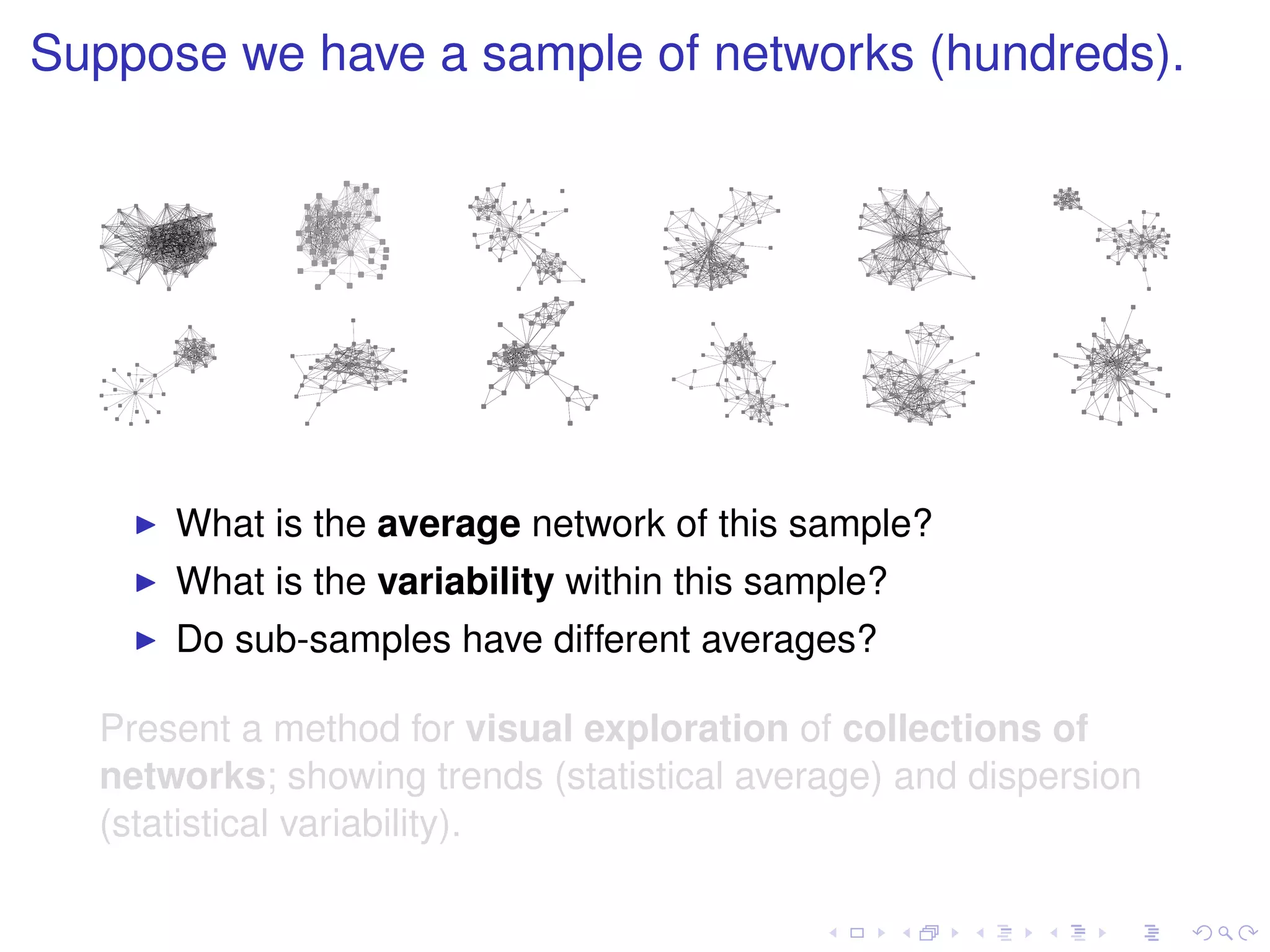
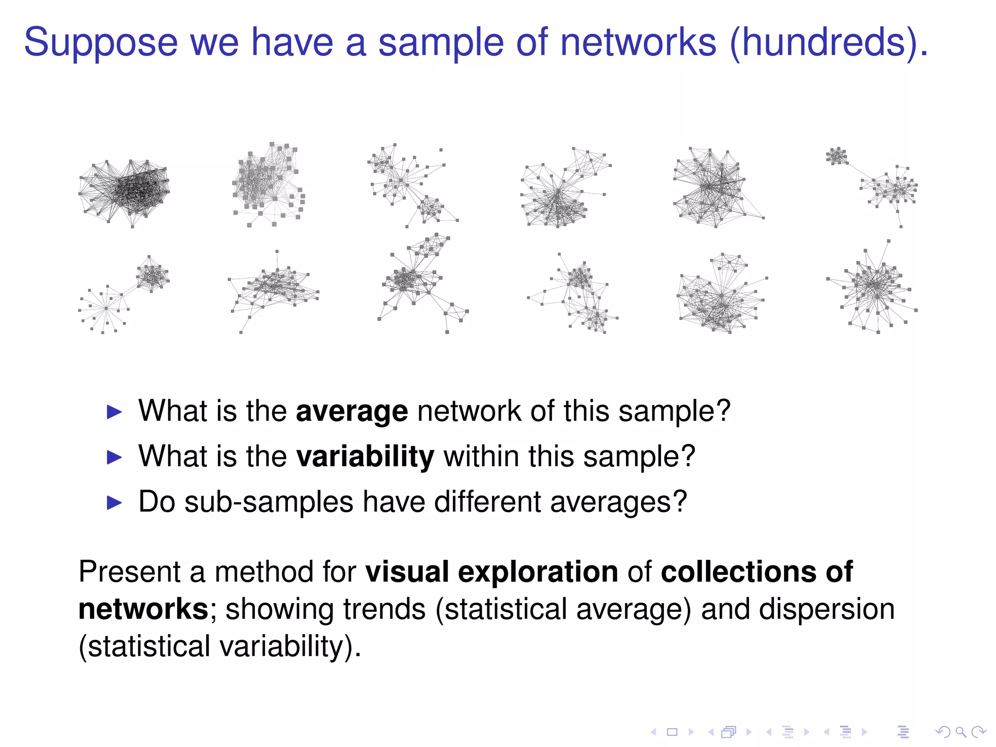
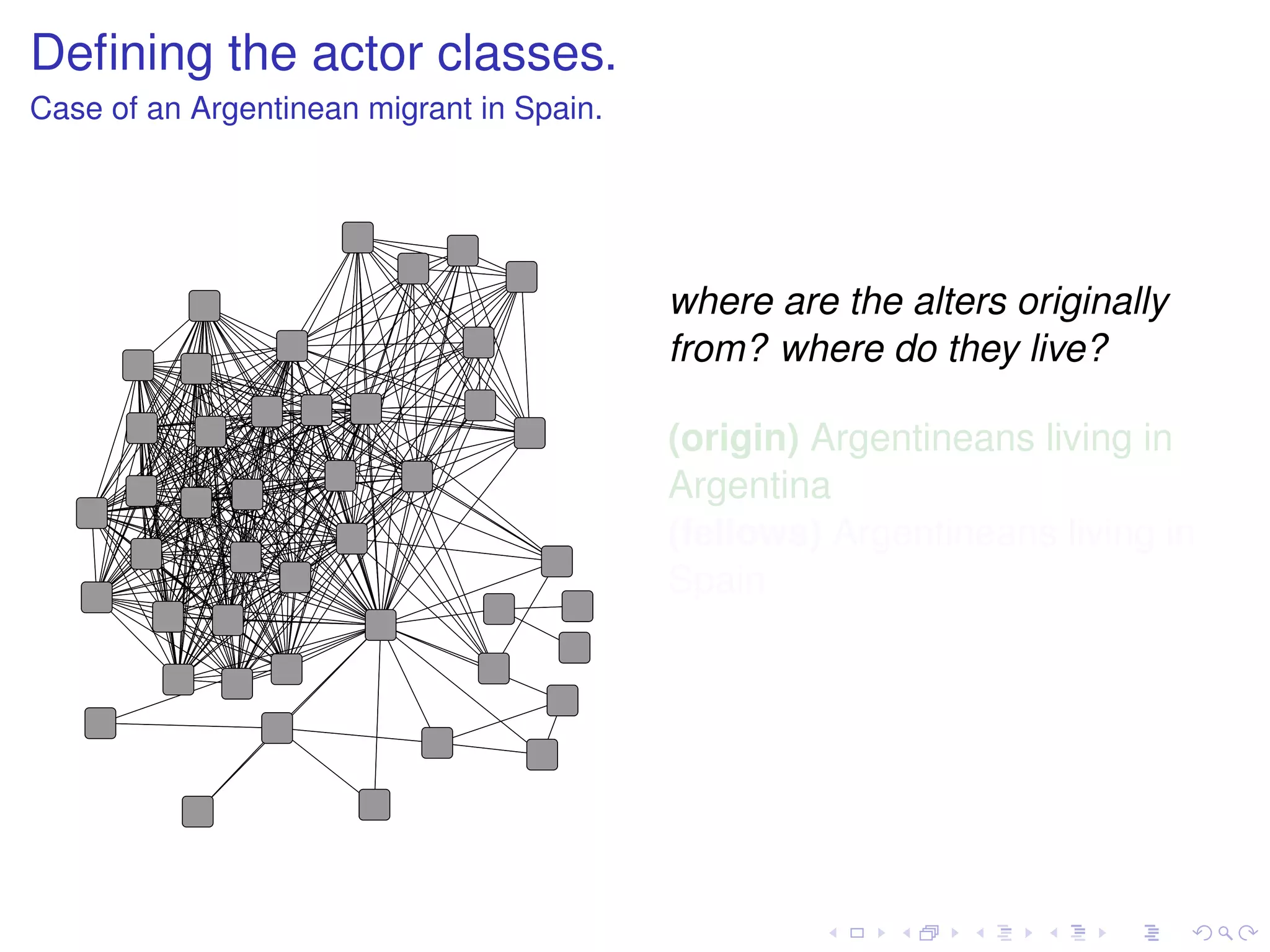
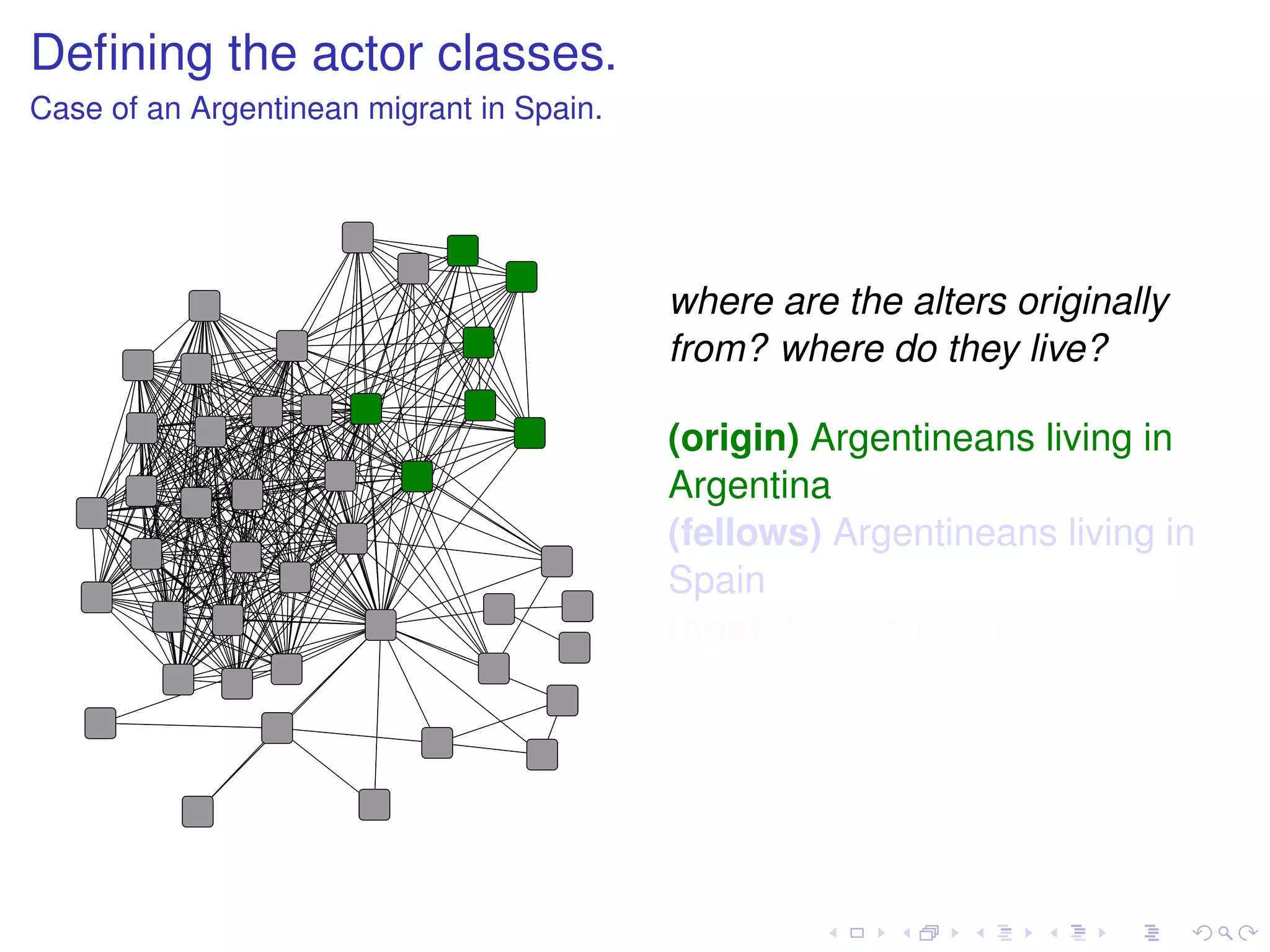
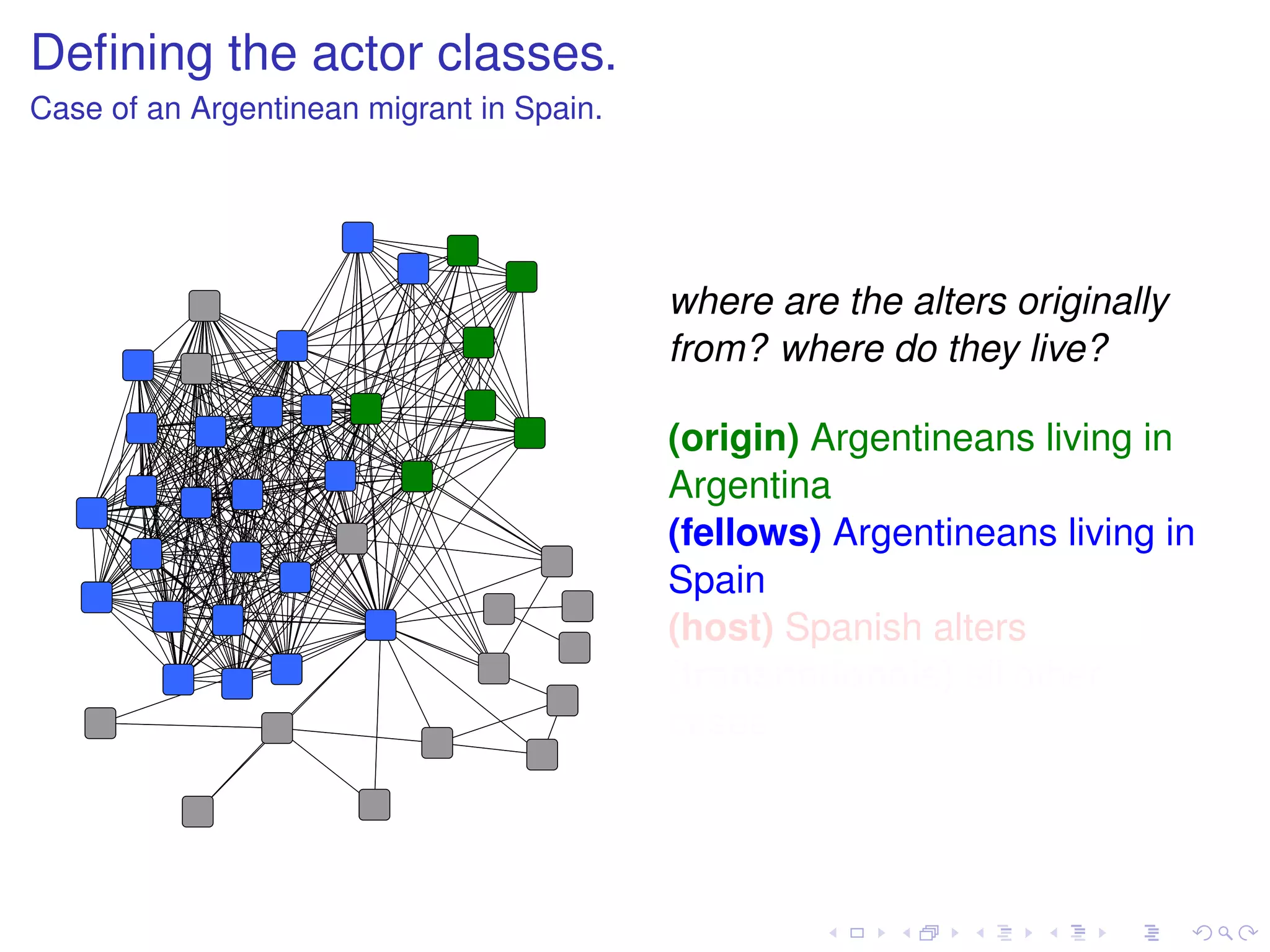
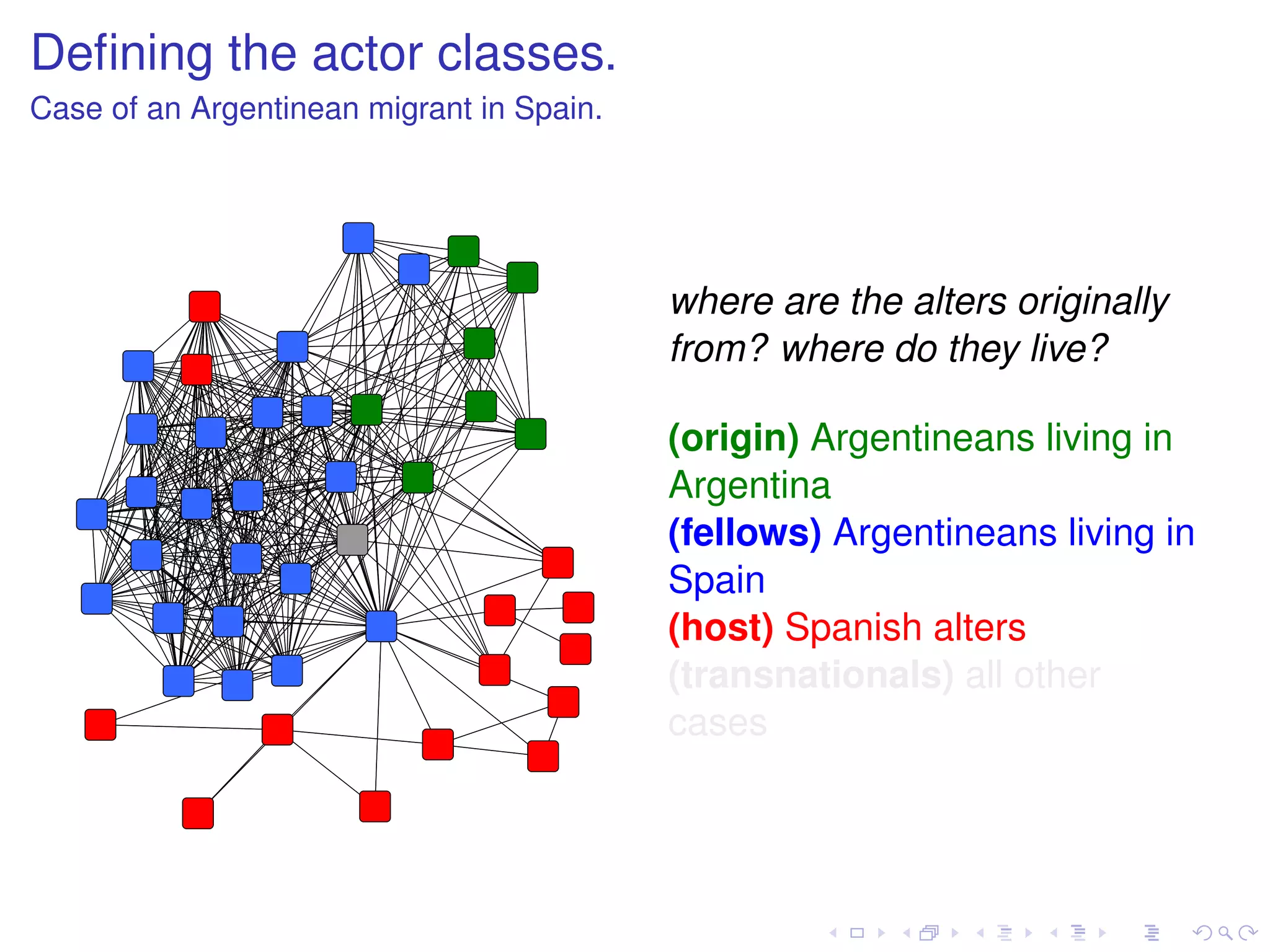
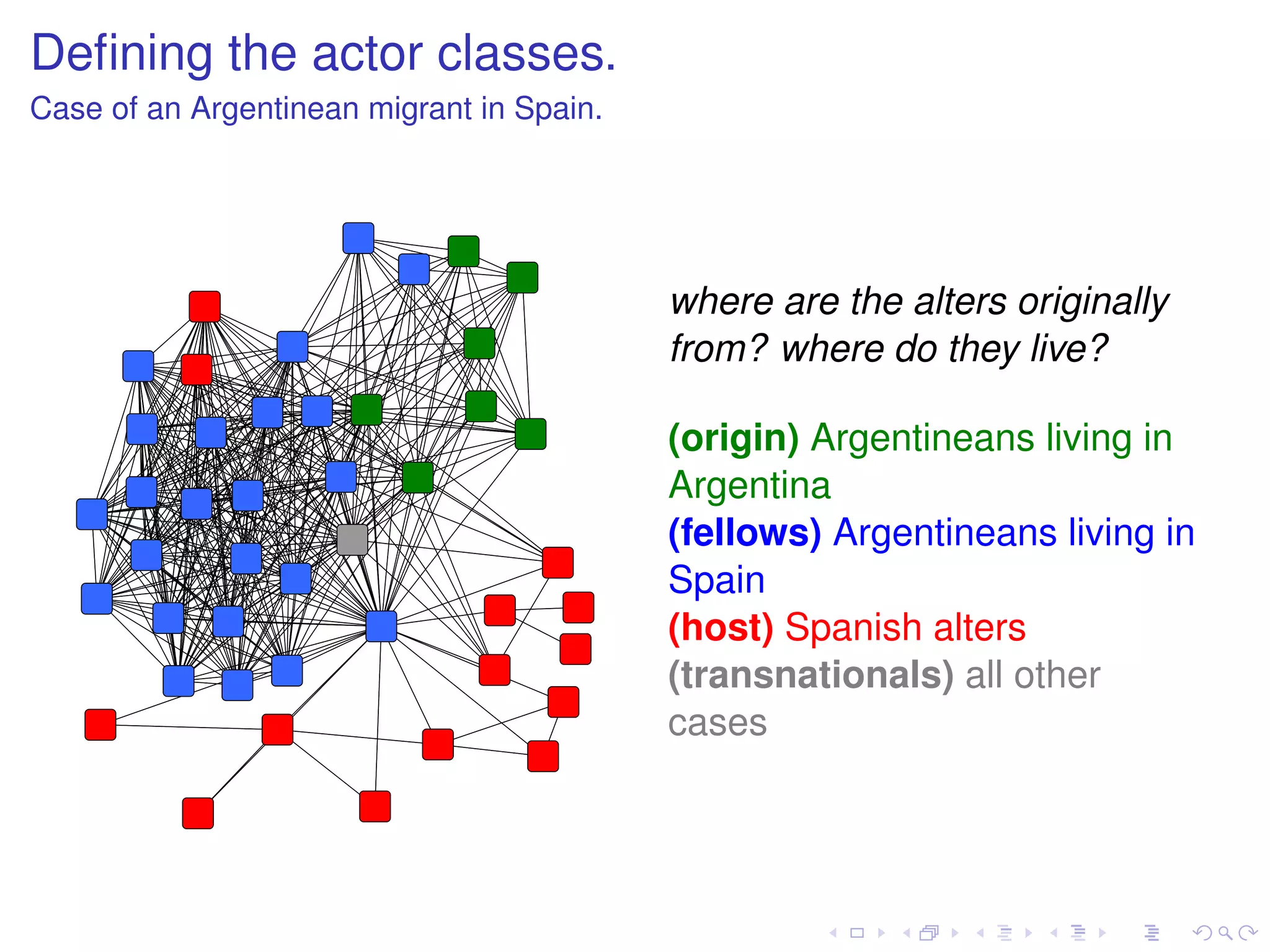
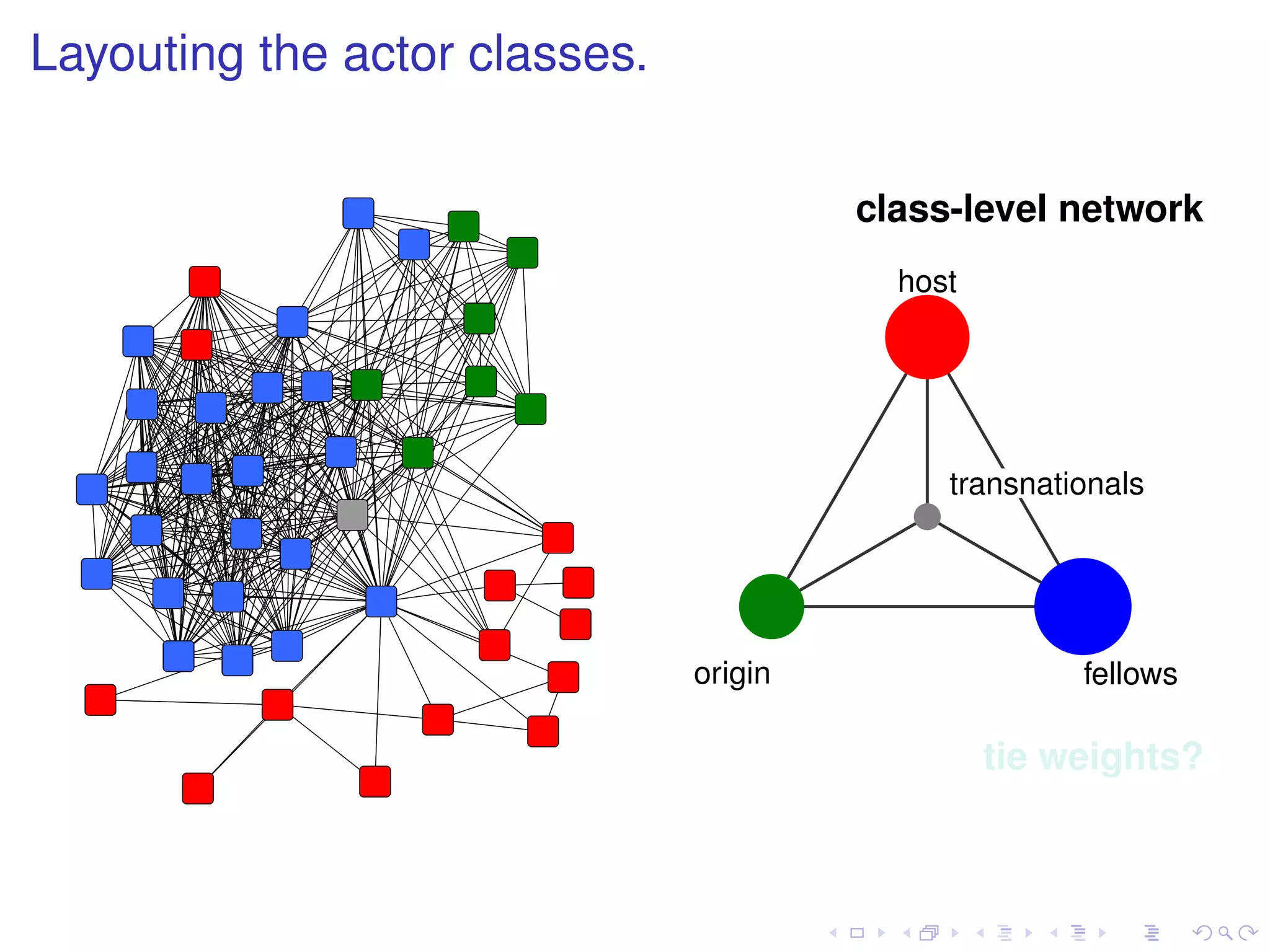
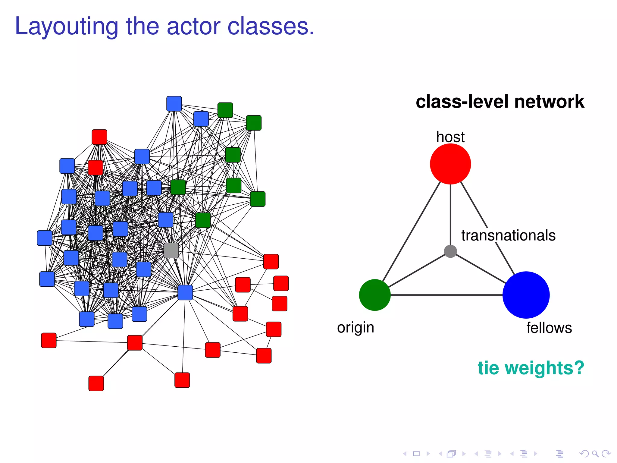
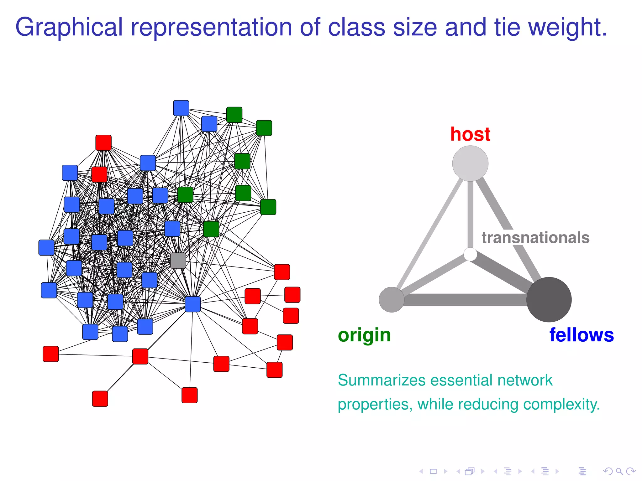
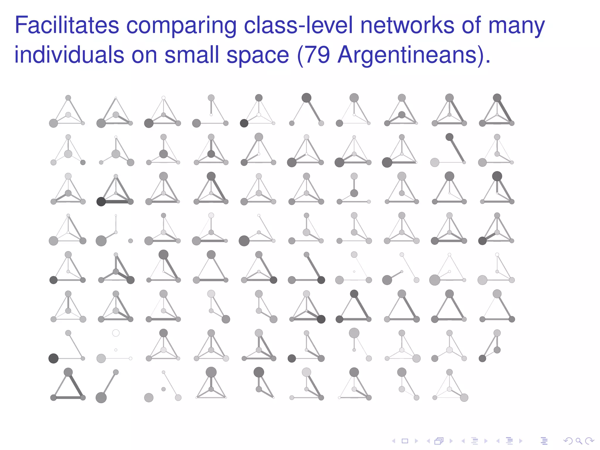
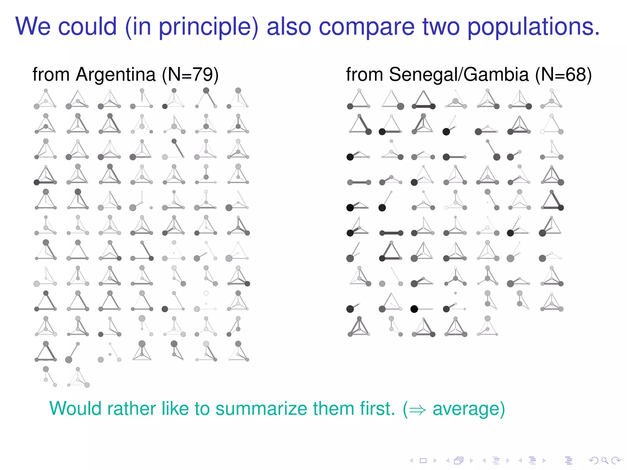
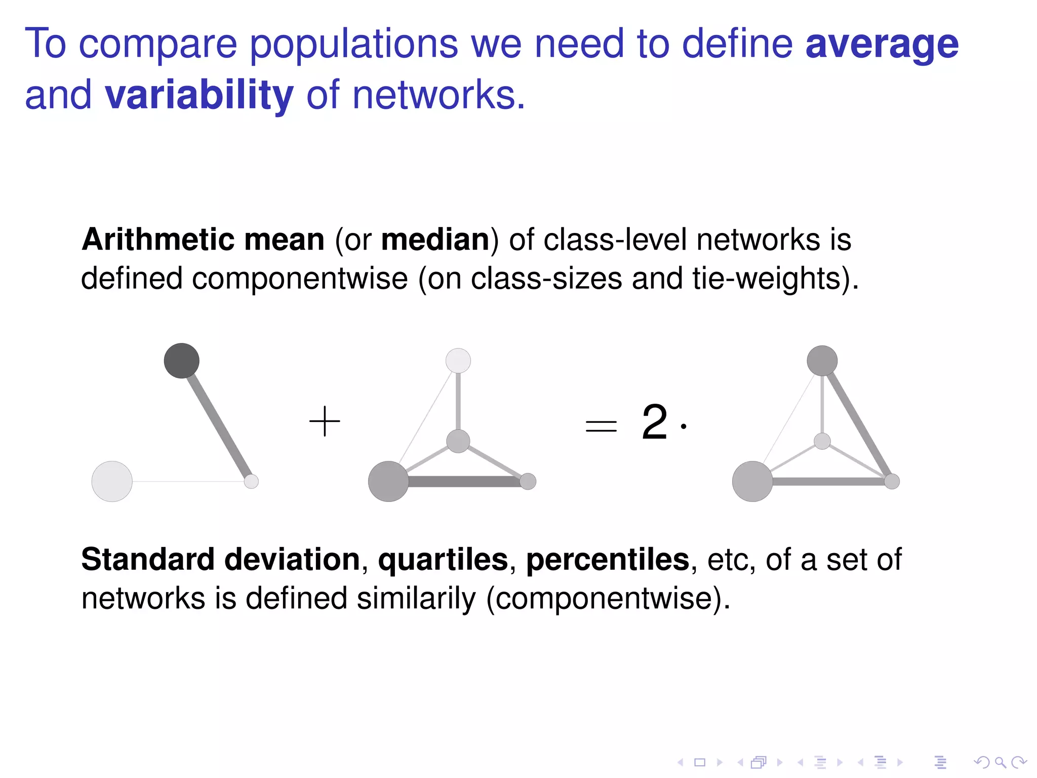
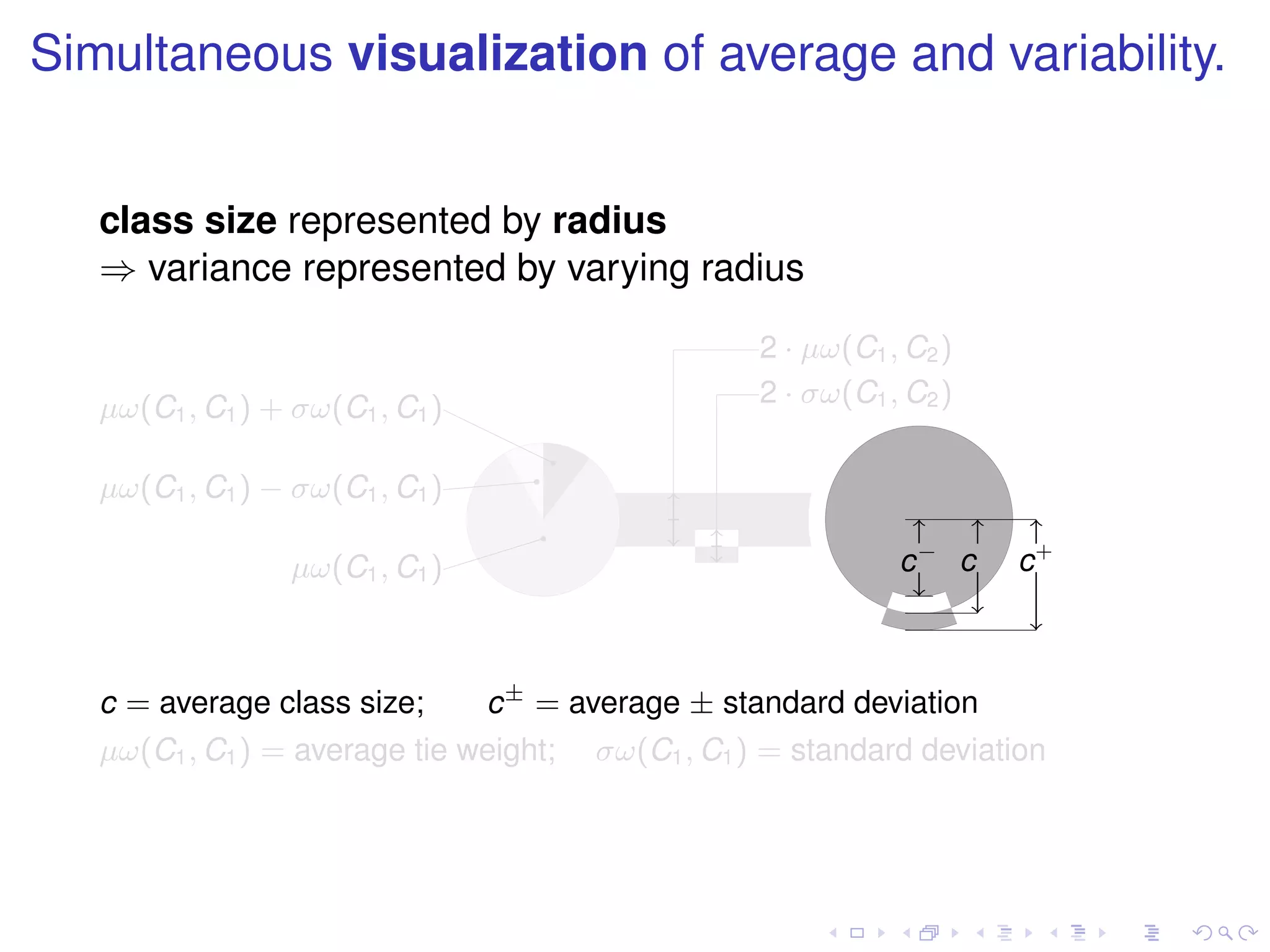
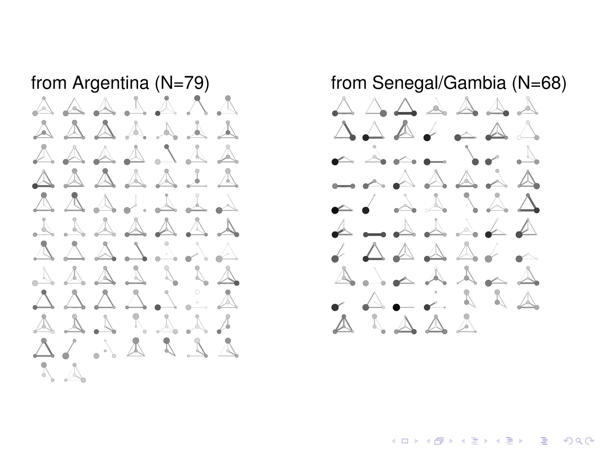
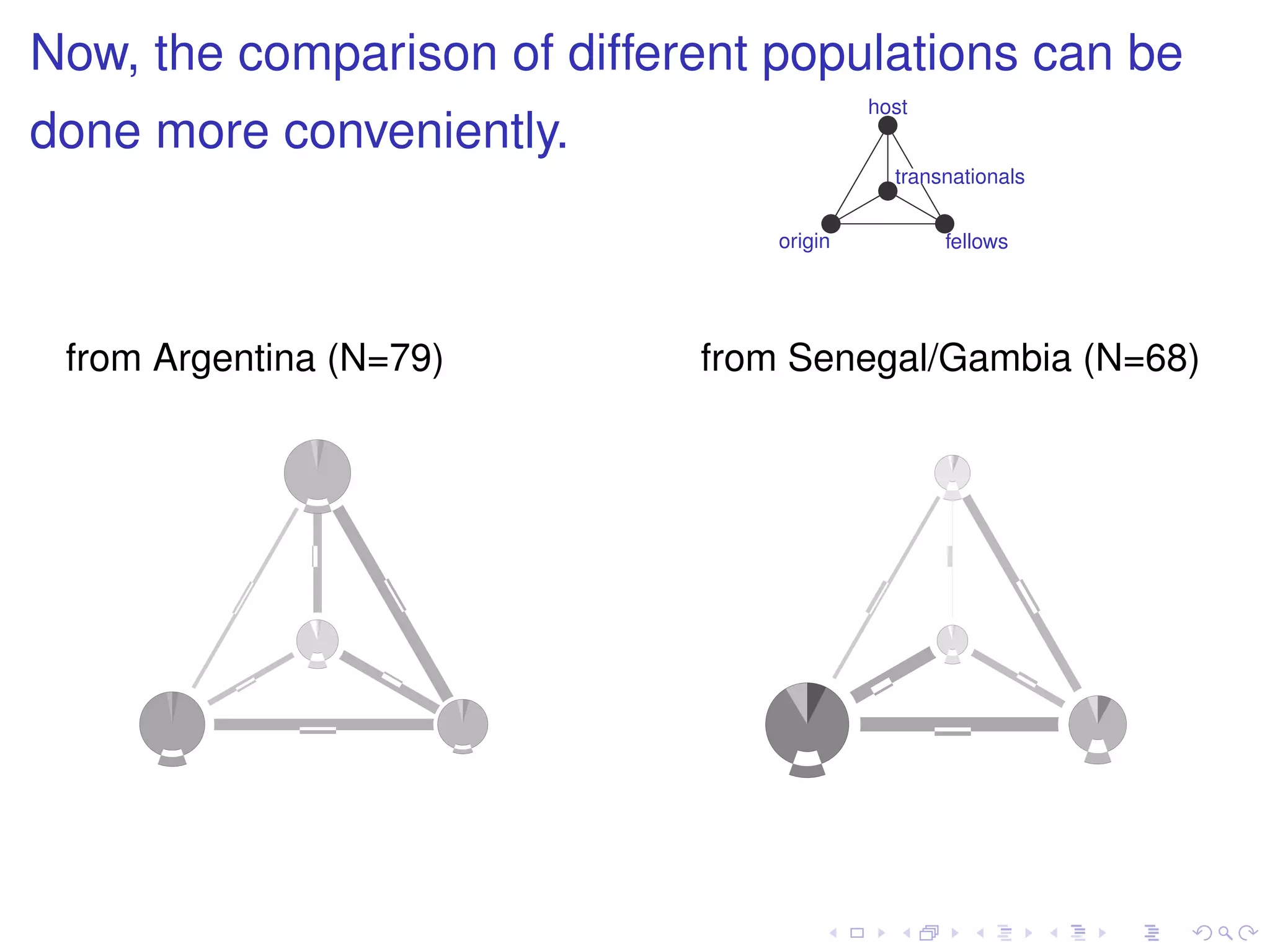
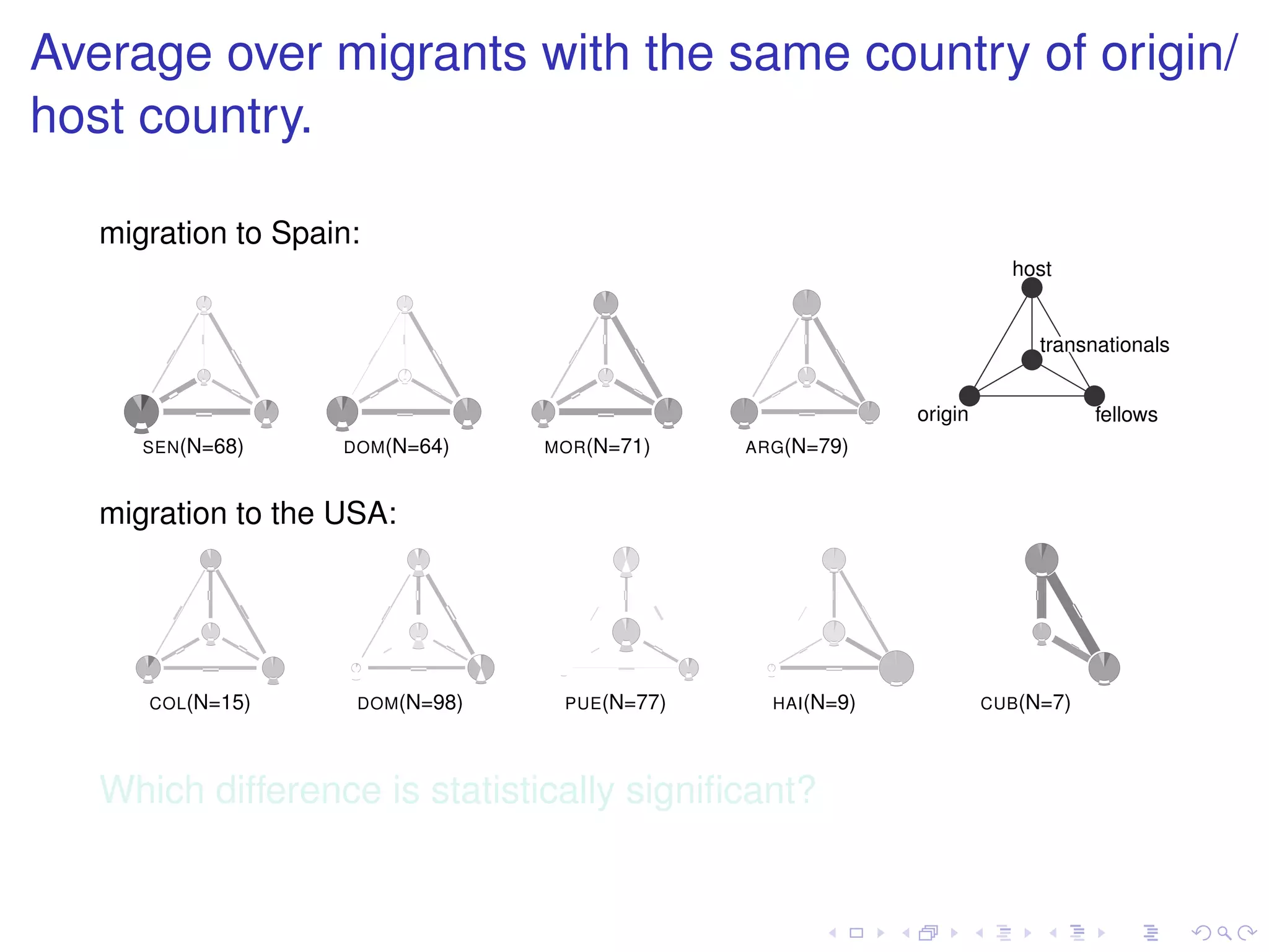
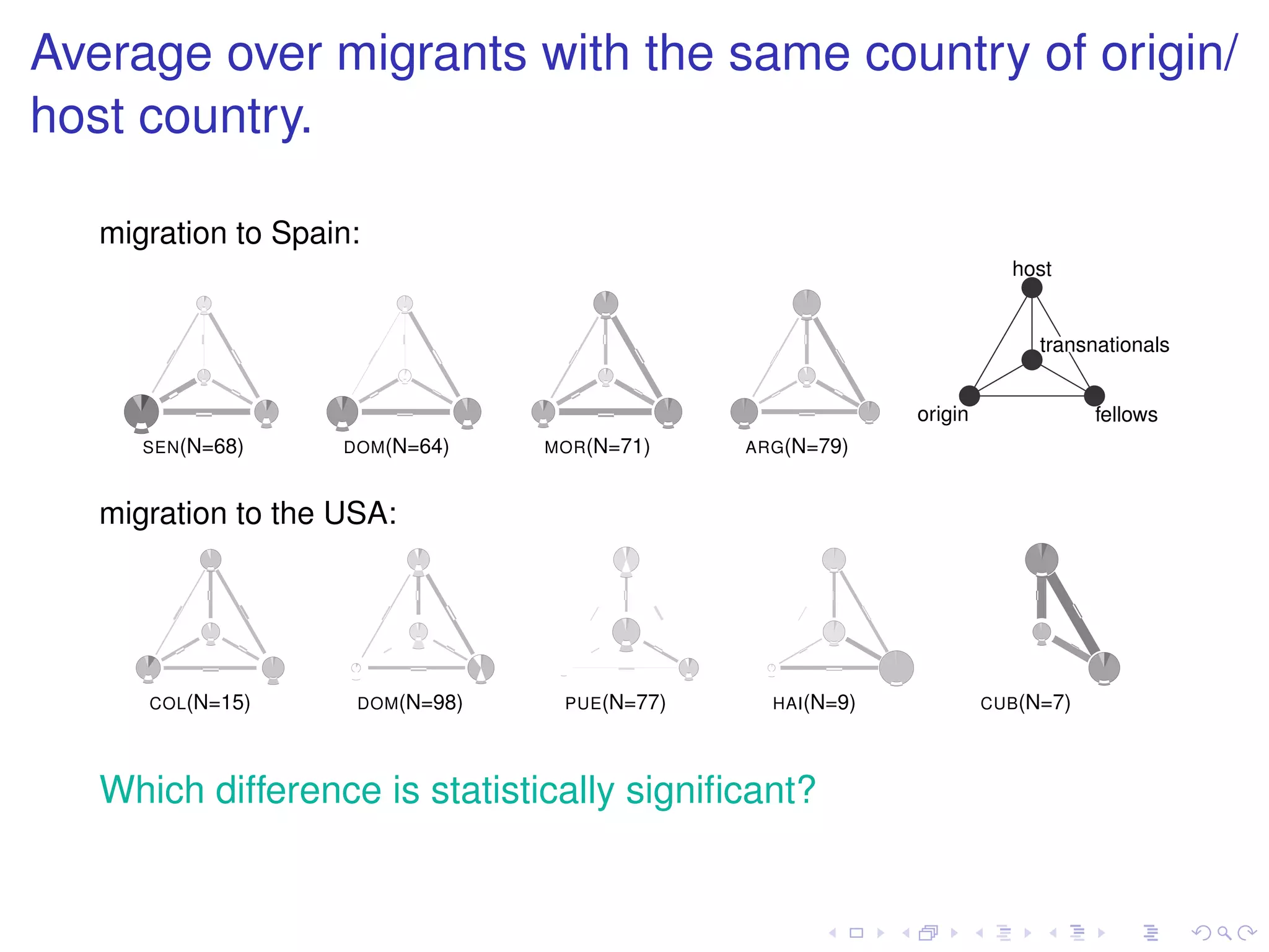
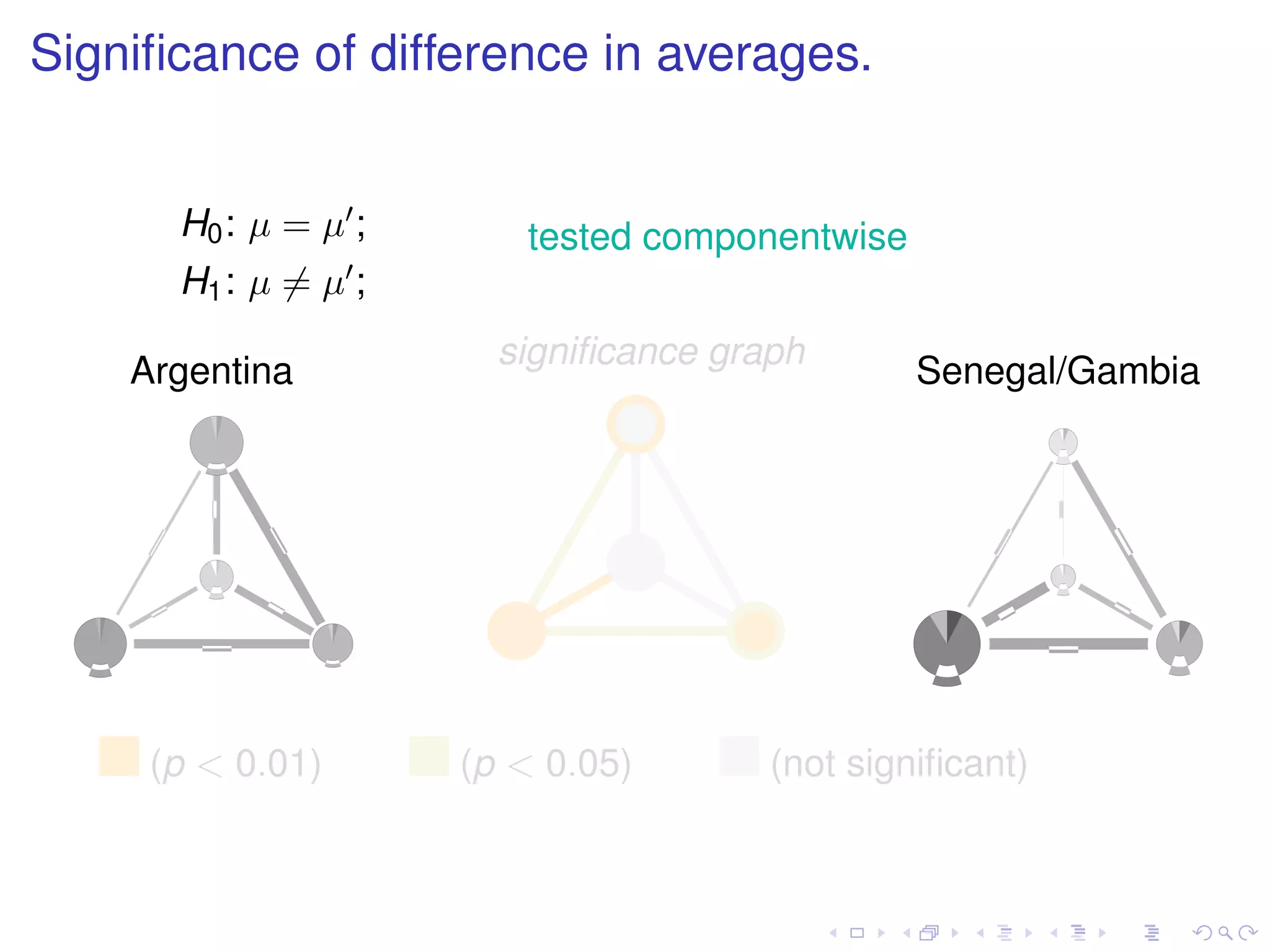
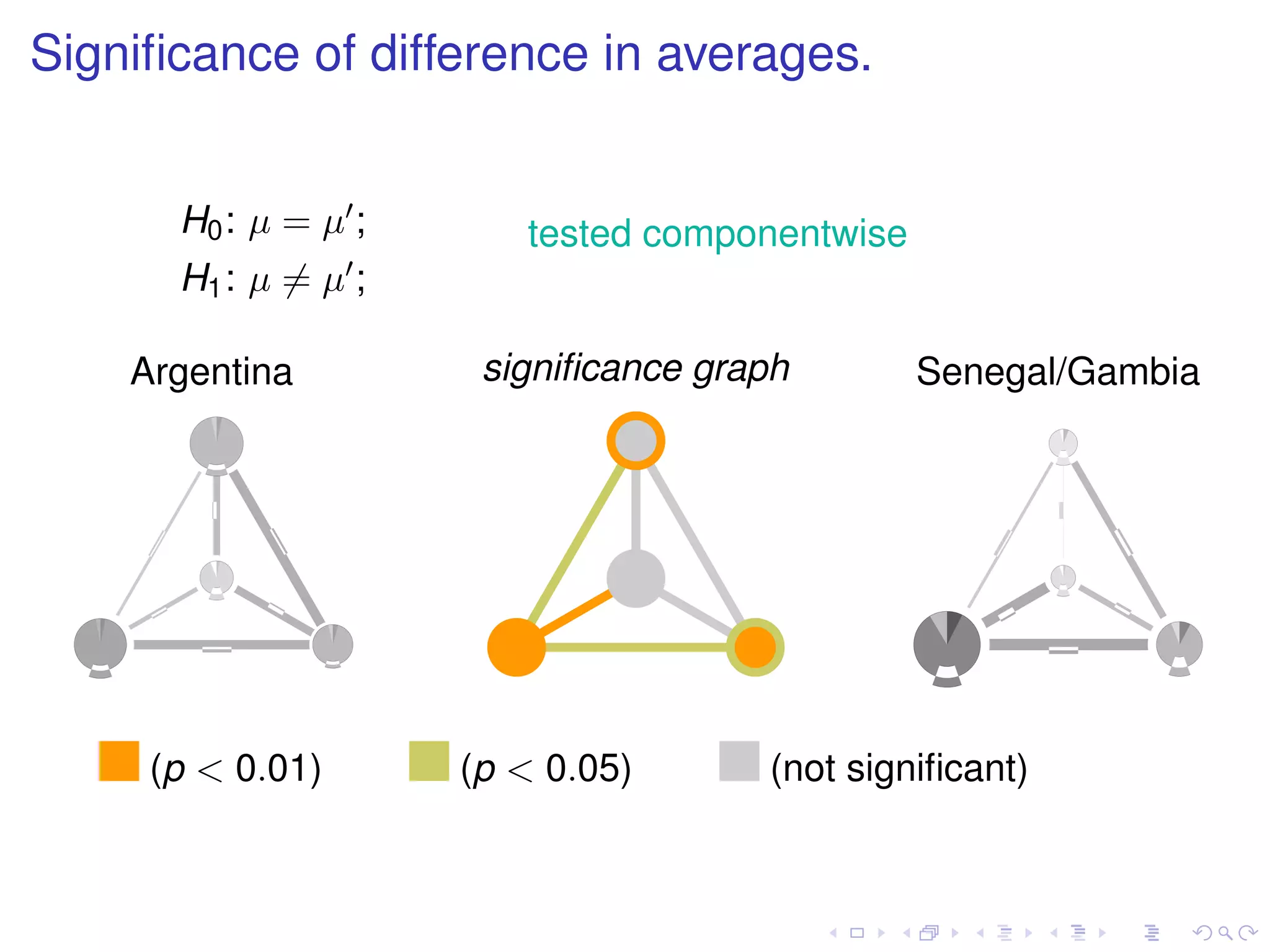
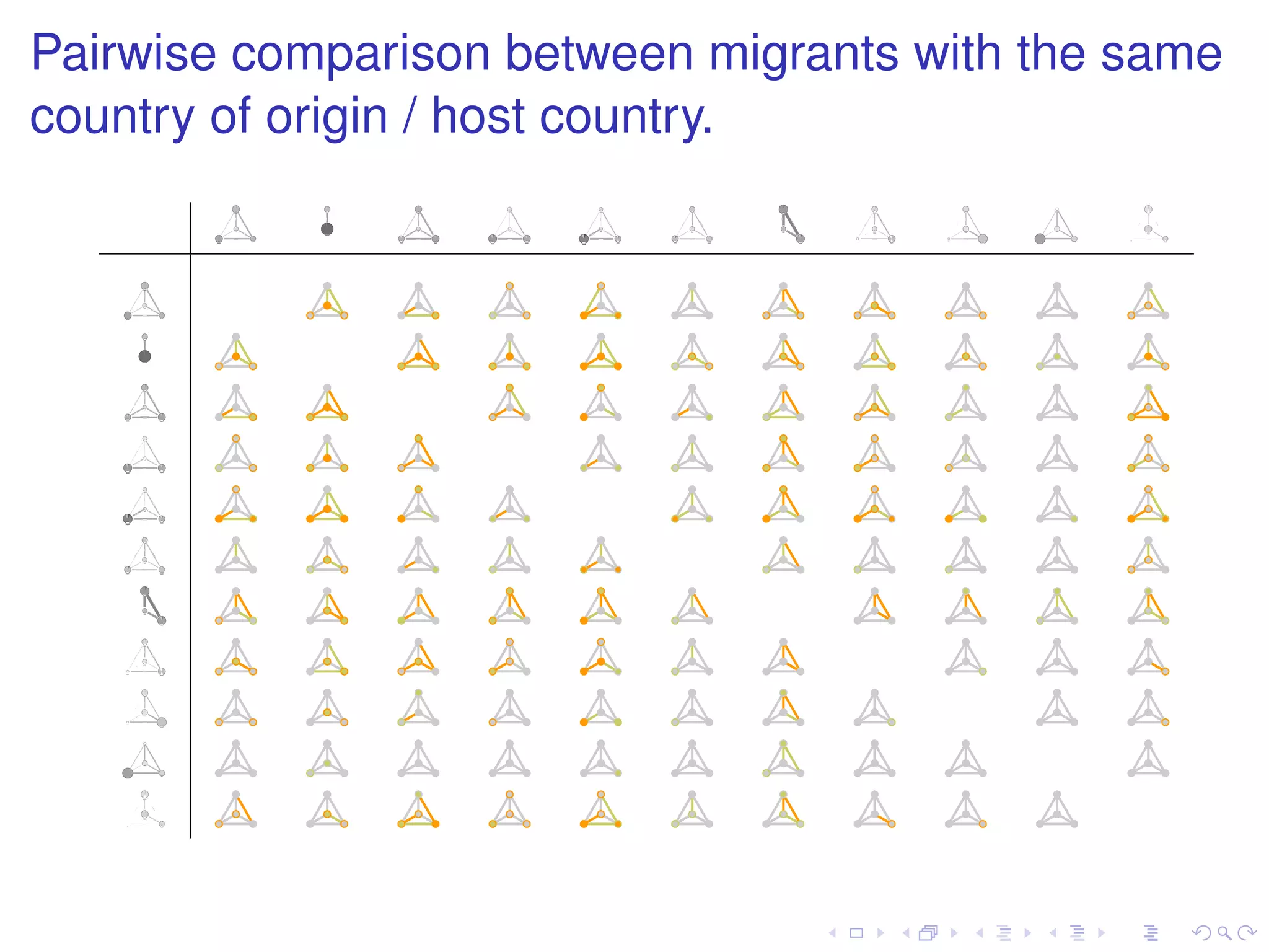
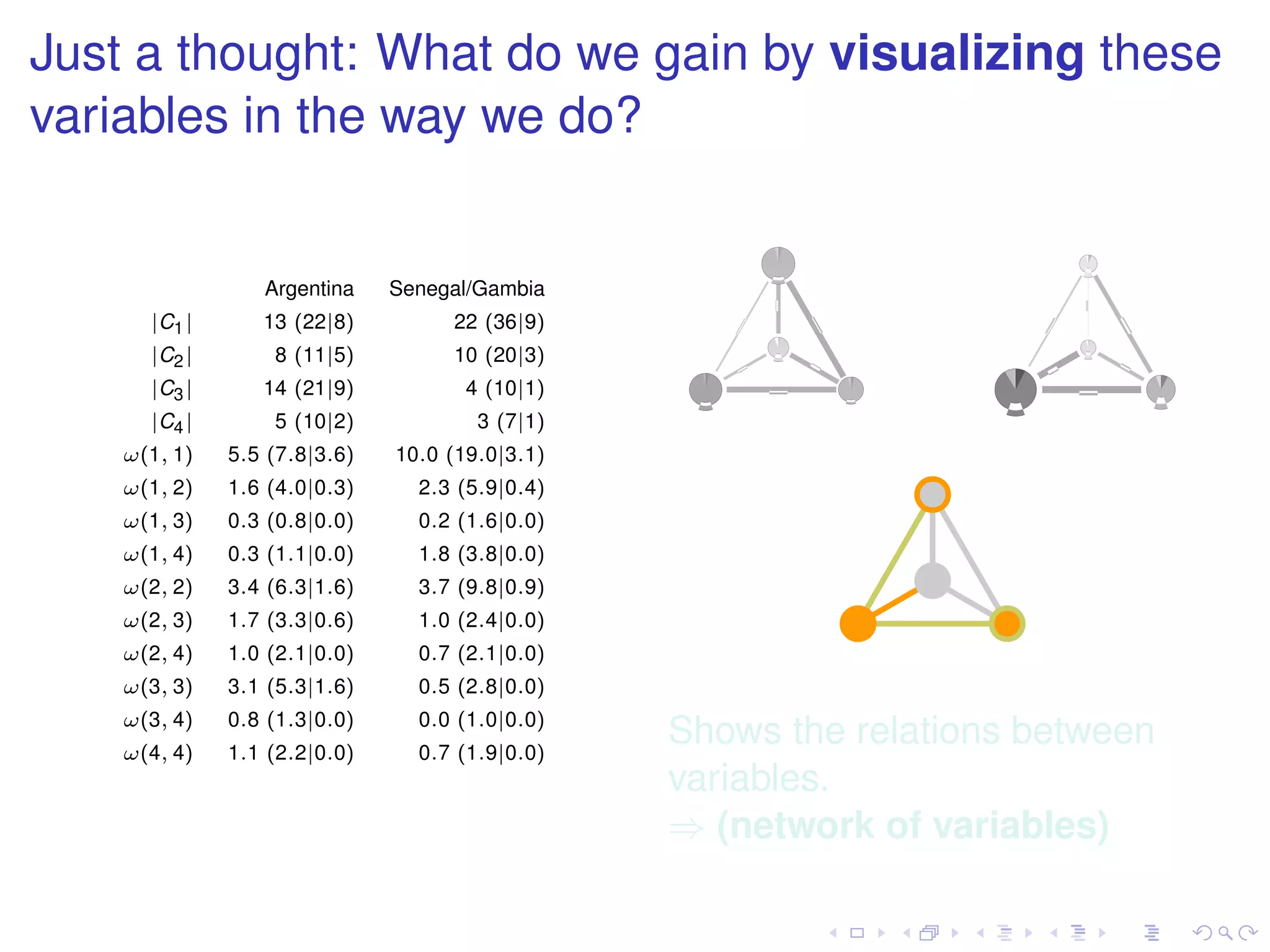
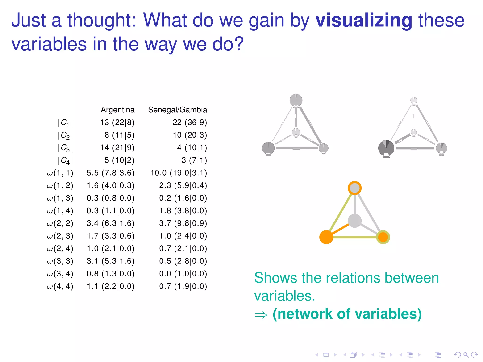
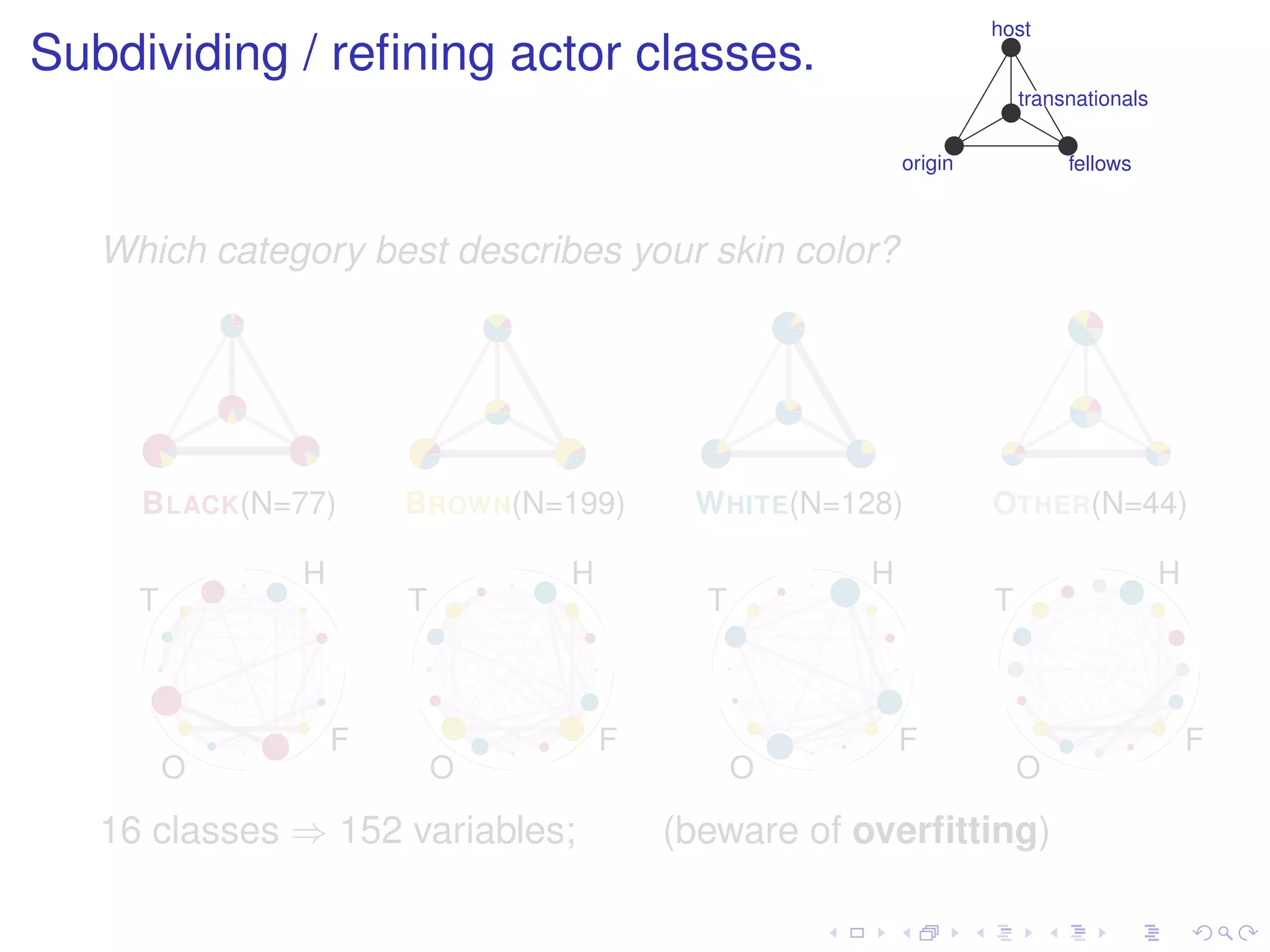
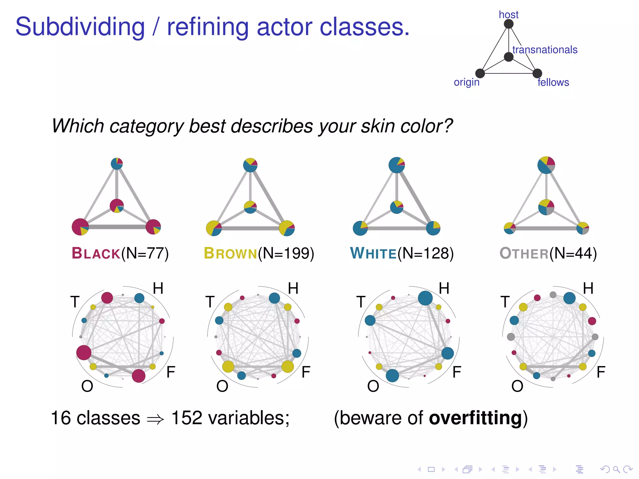
Visualizing Tendency and Dispersion in
         Collections of Attributed Networks

      Jürgen Lerner Ulrik Brandes Miranda J. Lubbers
              Chris McCarty José Luis Molina

            U. Konstanz    Autonomous U. Barcelona   U. Florida


XXVIII Sunbelt’08   St. Pete Beach                   January 22–27, 2008
Suppose we have a sample of networks (hundreds).


      What is the average network of this sample?
      What is the variability within this sample?
      Do sub-samples have different averages?

  Present a method for visual exploration of collections of
  networks; showing trends (statistical average) and dispersion
  (statistical variability).
Illustrate this approach on a concrete application.


   Understanding the acculturation of
   migrants by analyzing their personal
   networks.
   (Acculturation: outcome of cultures coming into contact.)
Empirical data set by interviewing ≈ 500 migrants in
Cataluña (Spain) and Florida (USA).

   From each respondent (ego) we got
    1. (questions about ego) country of origin, years of
       residence, skincolor, health, language skills, . . .
    2. (name generator) list of 45 alters
    3. (questions about alters) from, lives, skincolor, . . .
    4. (ties) which alters know each other


   Here: present visual exploration of this set of 500 networks.

   See www.egoredes.net for other work using this dataset.
Reduce networks of individuals to networks of classes.


   Two steps
    1. Define actor classes based on selected attributes.
    2. Define inter-class and intra-class ties (how strongly are two
       classes connected?).


   Benefits
       Reduction in size; small but informative images.
       Enables simple and efficient comparison between disjoint
       networks.
       Allows for averaging over collections of networks.
Defining the actor classes.
Case of an Argentinean migrant in Spain.


                                           where are the alters originally
                                           from? where do they live?

                                           (origin) Argentineans living in
                                           Argentina
                                           (fellows) Argentineans living in
                                           Spain
                                           (host) Spanish alters
                                           (transnationals) all other
                                           cases
Layouting the actor classes.


                                        class-level network
                                          host


                                             transnationals


                               origin                 fellows

                                                 tie weights?
Normalization of the tie weight.
How strongly are two classes connected?


    Given: network G = (V , E) and two actor classes A and B

      1. (un-normalized count)        #{(a, b) ∈ E ; a ∈ A, b ∈ B}
         ⇒ larger classes will be stronger connected
                       #{(a,b)∈E ; a∈A b∈B}
      2. (density)            |A|·|B|
         ⇒ tends to zero when class sizes increase (sparsity)
                                              #{(a,b)∈E ; a∈A b∈B}
      3. (avg. number of B-neighbors)                 |A|
         ⇒ asymmetric class-level network
                                          #{(a,b)∈E ; a∈A b∈B}
      4. (symmetric normalization)              √
                                                  |A|·|B|
         ⇒ this is what we take (appropriate for sparse networks)
Graphical representation of class size and tie weight.


                                             host


                                                 transnationals


                             origin                        fellows

                             Summarizes essential network
                             properties, while reducing complexity.
Facilitates comparing class-level networks of many
individuals on small space (79 Argentineans).
We could (in principle) also compare two populations.
 from Argentina (N=79)               from Senegal/Gambia (N=68)


   Would rather like to summarize them first. (⇒ average)
To compare populations we need to define average
and variability of networks.


  Arithmetic mean (or median) of class-level networks is
  defined componentwise (on class-sizes and tie-weights).


                  +                   = 2·

  Standard deviation, quartiles, percentiles, etc, of a set of
  networks is defined similarily (componentwise).
Simultaneous visualization of average and variability.


   class size represented by radius
   ⇒ variance represented by varying radius

                                                    2 · µω(C1 , C2 )
   µω(C1 , C1 ) + σω(C1 , C1 )                      2 · σω(C1 , C2 )


   µω(C1 , C1 ) − σω(C1 , C1 )

                  µω(C1 , C1 )                                 c− c+ c+


   c = average class size;       c ± = average ± standard deviation
   µω(C1 , C1 ) = average tie weight;   σω(C1 , C1 ) = standard deviation
Simultaneous visualization of average and variability.


   intra class tie weights represented by color (darkness)
   ⇒ variance represented by varying darkness

                                                    2 · µω(C1 , C2 )
   µω(C1 , C1 ) + σω(C1 , C1 )                      2 · σω(C1 , C2 )


   µω(C1 , C1 ) − σω(C1 , C1 )

                  µω(C1 , C1 )                                 c− c+ c+


   c = average class size;       c ± = average ± standard deviation
   µω(C1 , C1 ) = average tie weight;   σω(C1 , C1 ) = standard deviation
Simultaneous visualization of average and variability.


   inter class tie weights represented by edge thickness
   ⇒ variance represented by varying thickness

                                                    2 · µω(C1 , C2 )
   µω(C1 , C1 ) + σω(C1 , C1 )                      2 · σω(C1 , C2 )


   µω(C1 , C1 ) − σω(C1 , C1 )

                  µω(C1 , C1 )                                 c− c+ c+


   c = average class size;       c ± = average ± standard deviation
   µω(C1 , C1 ) = average tie weight;   σω(C1 , C1 ) = standard deviation
from Argentina (N=79)   from Senegal/Gambia (N=68)
Now, the comparison of different populations can be
                                          host
done more conveniently.
                                            transnationals


                                 origin          fellows


 from Argentina (N=79)       from Senegal/Gambia (N=68)
Average over migrants with the same country of origin/
host country.

   migration to Spain:
                                                                          host


                                                                            transnationals


                                                              origin               fellows
      SEN(N=68)     DOM (N=64)    MOR (N=71)    ARG (N=79)


   migration to the USA:


      COL(N=15)      DOM (N=98)    PUE (N=77)     HAI (N=9)            CUB (N=7)


   Which difference is statistically significant?
Significance of difference in averages.


      H0 : µ = µ ;      tested componentwise
      H1 : µ = µ ;
                       significance graph
    Argentina                                  Senegal/Gambia


     (p < 0.01)      (p < 0.05)       (not significant)
Significance of difference in averages.


      H0 : µ = µ ;      tested componentwise
      H1 : µ = µ ;

    Argentina         significance graph        Senegal/Gambia


     (p < 0.01)      (p < 0.05)      (not significant)
Pairwise comparison between migrants with the same
country of origin / host country.
Just a thought: What do we gain by visualizing these
variables in the way we do?


                 Argentina    Senegal/Gambia
      |C1 |      13 (22|8)         22 (36|9)
      |C2 |       8 (11|5)         10 (20|3)
      |C3 |      14 (21|9)           4 (10|1)
      |C4 |       5 (10|2)            3 (7|1)
    ω(1, 1)   5.5 (7.8|3.6)   10.0 (19.0|3.1)
    ω(1, 2)   1.6 (4.0|0.3)     2.3 (5.9|0.4)
    ω(1, 3)   0.3 (0.8|0.0)     0.2 (1.6|0.0)
    ω(1, 4)   0.3 (1.1|0.0)     1.8 (3.8|0.0)
    ω(2, 2)   3.4 (6.3|1.6)     3.7 (9.8|0.9)
    ω(2, 3)   1.7 (3.3|0.6)     1.0 (2.4|0.0)
    ω(2, 4)   1.0 (2.1|0.0)     0.7 (2.1|0.0)
    ω(3, 3)   3.1 (5.3|1.6)     0.5 (2.8|0.0)
    ω(3, 4)   0.8 (1.3|0.0)     0.0 (1.0|0.0)
    ω(4, 4)   1.1 (2.2|0.0)     0.7 (1.9|0.0)
                                                Shows the relations between
                                                variables.
                                                ⇒ (network of variables)
host
Subdividing / refining actor classes.
                                                                    transnationals


                                                       origin            fellows


   Which category best describes your skin color?


     B LACK(N=77)     B ROWN(N=199)     W HITE(N=128)           OTHER(N=44)

              H                H                   H                                 H
     T                T                  T                      T


                  F                F                   F                                 F
         O                O                  O                      O

   16 classes ⇒ 152 variables;         (beware of overfitting)
Conclusions.

  Presented a framework for averaging over collections of
  networks and for visualizing them.

       General applicability
             Suitable for all sets of networks with actor attributes.
             Efficient: suitable for large networks and many networks
             (small number of classes).

       Visualization is useful during analysis
           Large number of variables and relations between variables
         ⇒ keep the overview using appropriate network graphics.

  Further details in: Ulrik Brandes, Jürgen Lerner, Miranda J. Lubbers, Chris
  McCarty, and José Luis Molina. Visual Statistics for Collections of Clustered
  Graphs. In: Proc. IEEE Pacific Visualization Symp. (2008), to appear.

Clustered graphs

  • 1.
    Visualizing Tendency andDispersion in Collections of Attributed Networks Jürgen Lerner Ulrik Brandes Miranda J. Lubbers Chris McCarty José Luis Molina U. Konstanz Autonomous U. Barcelona U. Florida XXVIII Sunbelt’08 St. Pete Beach January 22–27, 2008
  • 2.
    Suppose we havea sample of networks (hundreds). What is the average network of this sample? What is the variability within this sample? Do sub-samples have different averages? Present a method for visual exploration of collections of networks; showing trends (statistical average) and dispersion (statistical variability).
  • 3.
    Suppose we havea sample of networks (hundreds). What is the average network of this sample? What is the variability within this sample? Do sub-samples have different averages? Present a method for visual exploration of collections of networks; showing trends (statistical average) and dispersion (statistical variability).
  • 4.
    Illustrate this approachon a concrete application. Understanding the acculturation of migrants by analyzing their personal networks. (Acculturation: outcome of cultures coming into contact.)
  • 5.
    Empirical data setby interviewing ≈ 500 migrants in Cataluña (Spain) and Florida (USA). From each respondent (ego) we got 1. (questions about ego) country of origin, years of residence, skincolor, health, language skills, . . . 2. (name generator) list of 45 alters 3. (questions about alters) from, lives, skincolor, . . . 4. (ties) which alters know each other Here: present visual exploration of this set of 500 networks. See www.egoredes.net for other work using this dataset.
  • 6.
    Reduce networks ofindividuals to networks of classes. Two steps 1. Define actor classes based on selected attributes. 2. Define inter-class and intra-class ties (how strongly are two classes connected?). Benefits Reduction in size; small but informative images. Enables simple and efficient comparison between disjoint networks. Allows for averaging over collections of networks.
  • 7.
    Reduce networks ofindividuals to networks of classes. Two steps 1. Define actor classes based on selected attributes. 2. Define inter-class and intra-class ties (how strongly are two classes connected?). Benefits Reduction in size; small but informative images. Enables simple and efficient comparison between disjoint networks. Allows for averaging over collections of networks.
  • 8.
    Defining the actorclasses. Case of an Argentinean migrant in Spain. where are the alters originally from? where do they live? (origin) Argentineans living in Argentina (fellows) Argentineans living in Spain (host) Spanish alters (transnationals) all other cases
  • 9.
    Defining the actorclasses. Case of an Argentinean migrant in Spain. where are the alters originally from? where do they live? (origin) Argentineans living in Argentina (fellows) Argentineans living in Spain (host) Spanish alters (transnationals) all other cases
  • 10.
    Defining the actorclasses. Case of an Argentinean migrant in Spain. where are the alters originally from? where do they live? (origin) Argentineans living in Argentina (fellows) Argentineans living in Spain (host) Spanish alters (transnationals) all other cases
  • 11.
    Defining the actorclasses. Case of an Argentinean migrant in Spain. where are the alters originally from? where do they live? (origin) Argentineans living in Argentina (fellows) Argentineans living in Spain (host) Spanish alters (transnationals) all other cases
  • 12.
    Defining the actorclasses. Case of an Argentinean migrant in Spain. where are the alters originally from? where do they live? (origin) Argentineans living in Argentina (fellows) Argentineans living in Spain (host) Spanish alters (transnationals) all other cases
  • 13.
    Layouting the actorclasses. class-level network host transnationals origin fellows tie weights?
  • 14.
    Layouting the actorclasses. class-level network host transnationals origin fellows tie weights?
  • 15.
    Normalization of thetie weight. How strongly are two classes connected? Given: network G = (V , E) and two actor classes A and B 1. (un-normalized count) #{(a, b) ∈ E ; a ∈ A, b ∈ B} ⇒ larger classes will be stronger connected #{(a,b)∈E ; a∈A b∈B} 2. (density) |A|·|B| ⇒ tends to zero when class sizes increase (sparsity) #{(a,b)∈E ; a∈A b∈B} 3. (avg. number of B-neighbors) |A| ⇒ asymmetric class-level network #{(a,b)∈E ; a∈A b∈B} 4. (symmetric normalization) √ |A|·|B| ⇒ this is what we take (appropriate for sparse networks)
  • 16.
    Graphical representation ofclass size and tie weight. host transnationals origin fellows Summarizes essential network properties, while reducing complexity.
  • 17.
    Facilitates comparing class-levelnetworks of many individuals on small space (79 Argentineans).
  • 18.
    We could (inprinciple) also compare two populations. from Argentina (N=79) from Senegal/Gambia (N=68) Would rather like to summarize them first. (⇒ average)
  • 19.
    To compare populationswe need to define average and variability of networks. Arithmetic mean (or median) of class-level networks is defined componentwise (on class-sizes and tie-weights). + = 2· Standard deviation, quartiles, percentiles, etc, of a set of networks is defined similarily (componentwise).
  • 20.
    To compare populationswe need to define average and variability of networks. Arithmetic mean (or median) of class-level networks is defined componentwise (on class-sizes and tie-weights). + = 2· Standard deviation, quartiles, percentiles, etc, of a set of networks is defined similarily (componentwise).
  • 21.
    Simultaneous visualization ofaverage and variability. class size represented by radius ⇒ variance represented by varying radius 2 · µω(C1 , C2 ) µω(C1 , C1 ) + σω(C1 , C1 ) 2 · σω(C1 , C2 ) µω(C1 , C1 ) − σω(C1 , C1 ) µω(C1 , C1 ) c− c+ c+ c = average class size; c ± = average ± standard deviation µω(C1 , C1 ) = average tie weight; σω(C1 , C1 ) = standard deviation
  • 22.
    Simultaneous visualization ofaverage and variability. intra class tie weights represented by color (darkness) ⇒ variance represented by varying darkness 2 · µω(C1 , C2 ) µω(C1 , C1 ) + σω(C1 , C1 ) 2 · σω(C1 , C2 ) µω(C1 , C1 ) − σω(C1 , C1 ) µω(C1 , C1 ) c− c+ c+ c = average class size; c ± = average ± standard deviation µω(C1 , C1 ) = average tie weight; σω(C1 , C1 ) = standard deviation
  • 23.
    Simultaneous visualization ofaverage and variability. inter class tie weights represented by edge thickness ⇒ variance represented by varying thickness 2 · µω(C1 , C2 ) µω(C1 , C1 ) + σω(C1 , C1 ) 2 · σω(C1 , C2 ) µω(C1 , C1 ) − σω(C1 , C1 ) µω(C1 , C1 ) c− c+ c+ c = average class size; c ± = average ± standard deviation µω(C1 , C1 ) = average tie weight; σω(C1 , C1 ) = standard deviation
  • 24.
    from Argentina (N=79) from Senegal/Gambia (N=68)
  • 25.
    Now, the comparisonof different populations can be host done more conveniently. transnationals origin fellows from Argentina (N=79) from Senegal/Gambia (N=68)
  • 26.
    Average over migrantswith the same country of origin/ host country. migration to Spain: host transnationals origin fellows SEN(N=68) DOM (N=64) MOR (N=71) ARG (N=79) migration to the USA: COL(N=15) DOM (N=98) PUE (N=77) HAI (N=9) CUB (N=7) Which difference is statistically significant?
  • 27.
    Average over migrantswith the same country of origin/ host country. migration to Spain: host transnationals origin fellows SEN(N=68) DOM (N=64) MOR (N=71) ARG (N=79) migration to the USA: COL(N=15) DOM (N=98) PUE (N=77) HAI (N=9) CUB (N=7) Which difference is statistically significant?
  • 28.
    Significance of differencein averages. H0 : µ = µ ; tested componentwise H1 : µ = µ ; significance graph Argentina Senegal/Gambia (p < 0.01) (p < 0.05) (not significant)
  • 29.
    Significance of differencein averages. H0 : µ = µ ; tested componentwise H1 : µ = µ ; Argentina significance graph Senegal/Gambia (p < 0.01) (p < 0.05) (not significant)
  • 30.
    Pairwise comparison betweenmigrants with the same country of origin / host country.
  • 31.
    Just a thought:What do we gain by visualizing these variables in the way we do? Argentina Senegal/Gambia |C1 | 13 (22|8) 22 (36|9) |C2 | 8 (11|5) 10 (20|3) |C3 | 14 (21|9) 4 (10|1) |C4 | 5 (10|2) 3 (7|1) ω(1, 1) 5.5 (7.8|3.6) 10.0 (19.0|3.1) ω(1, 2) 1.6 (4.0|0.3) 2.3 (5.9|0.4) ω(1, 3) 0.3 (0.8|0.0) 0.2 (1.6|0.0) ω(1, 4) 0.3 (1.1|0.0) 1.8 (3.8|0.0) ω(2, 2) 3.4 (6.3|1.6) 3.7 (9.8|0.9) ω(2, 3) 1.7 (3.3|0.6) 1.0 (2.4|0.0) ω(2, 4) 1.0 (2.1|0.0) 0.7 (2.1|0.0) ω(3, 3) 3.1 (5.3|1.6) 0.5 (2.8|0.0) ω(3, 4) 0.8 (1.3|0.0) 0.0 (1.0|0.0) ω(4, 4) 1.1 (2.2|0.0) 0.7 (1.9|0.0) Shows the relations between variables. ⇒ (network of variables)
  • 32.
    Just a thought:What do we gain by visualizing these variables in the way we do? Argentina Senegal/Gambia |C1 | 13 (22|8) 22 (36|9) |C2 | 8 (11|5) 10 (20|3) |C3 | 14 (21|9) 4 (10|1) |C4 | 5 (10|2) 3 (7|1) ω(1, 1) 5.5 (7.8|3.6) 10.0 (19.0|3.1) ω(1, 2) 1.6 (4.0|0.3) 2.3 (5.9|0.4) ω(1, 3) 0.3 (0.8|0.0) 0.2 (1.6|0.0) ω(1, 4) 0.3 (1.1|0.0) 1.8 (3.8|0.0) ω(2, 2) 3.4 (6.3|1.6) 3.7 (9.8|0.9) ω(2, 3) 1.7 (3.3|0.6) 1.0 (2.4|0.0) ω(2, 4) 1.0 (2.1|0.0) 0.7 (2.1|0.0) ω(3, 3) 3.1 (5.3|1.6) 0.5 (2.8|0.0) ω(3, 4) 0.8 (1.3|0.0) 0.0 (1.0|0.0) ω(4, 4) 1.1 (2.2|0.0) 0.7 (1.9|0.0) Shows the relations between variables. ⇒ (network of variables)
  • 33.
    host Subdividing / refiningactor classes. transnationals origin fellows Which category best describes your skin color? B LACK(N=77) B ROWN(N=199) W HITE(N=128) OTHER(N=44) H H H H T T T T F F F F O O O O 16 classes ⇒ 152 variables; (beware of overfitting)
  • 34.
    host Subdividing / refiningactor classes. transnationals origin fellows Which category best describes your skin color? B LACK(N=77) B ROWN(N=199) W HITE(N=128) OTHER(N=44) H H H H T T T T F F F F O O O O 16 classes ⇒ 152 variables; (beware of overfitting)
  • 35.
    host Subdividing / refiningactor classes. transnationals origin fellows Which category best describes your skin color? B LACK(N=77) B ROWN(N=199) W HITE(N=128) OTHER(N=44) H H H H T T T T F F F F O O O O 16 classes ⇒ 152 variables; (beware of overfitting)
  • 36.
    host Subdividing / refiningactor classes. transnationals origin fellows Which category best describes your skin color? B LACK(N=77) B ROWN(N=199) W HITE(N=128) OTHER(N=44) H H H H T T T T F F F F O O O O 16 classes ⇒ 152 variables; (beware of overfitting)
  • 37.
    host Subdividing / refiningactor classes. transnationals origin fellows Which category best describes your skin color? B LACK(N=77) B ROWN(N=199) W HITE(N=128) OTHER(N=44) H H H H T T T T F F F F O O O O 16 classes ⇒ 152 variables; (beware of overfitting)
  • 38.
    Conclusions. Presenteda framework for averaging over collections of networks and for visualizing them. General applicability Suitable for all sets of networks with actor attributes. Efficient: suitable for large networks and many networks (small number of classes). Visualization is useful during analysis Large number of variables and relations between variables ⇒ keep the overview using appropriate network graphics. Further details in: Ulrik Brandes, Jürgen Lerner, Miranda J. Lubbers, Chris McCarty, and José Luis Molina. Visual Statistics for Collections of Clustered Graphs. In: Proc. IEEE Pacific Visualization Symp. (2008), to appear.