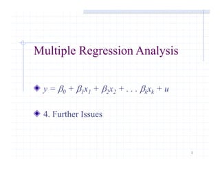
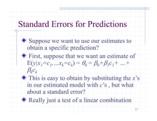
This document provides an overview of multiple regression analysis and common issues that arise. It discusses how changing the scale of variables affects coefficients, the meaning of beta coefficients, using nonlinear transformations like logs and quadratic terms, interpreting coefficients in log models, and various diagnostics like adjusted R-squared and residual analysis. Guidelines are also given for predicting values and comparing log versus level models.

1. 1
Multiple Regression Analysis
y = 0 + 1x1 + 2x2 + . . . kxk + u
4. Further Issues

2. 2
Redefining Variables
Changing the scale of the y variable will
lead to a corresponding change in the scale
of the coefficients and standard errors, so no
change in the significance or interpretation
Changing the scale of one x variable will
lead to a change in the scale of that
coefficient and standard error, so no change
in the significance or interpretation

3. 3
Beta Coefficients
Occasional you’ll see reference to a
“standardized coefficient” or “beta
coefficient” which has a specific meaning
Idea is to replace y and each x variable with
a standardized version – i.e. subtract mean
and divide by standard deviation
Coefficient reflects standard deviation of y
for a one standard deviation change in x

4. 4
Functional Form
OLS can be used for relationships that are
not strictly linear in x and y by using
nonlinear functions of x and y – will still be
linear in the parameters
Can take the natural log of x, y or both
Can use quadratic forms of x
Can use interactions of x variables

5. 5
Interpretation of Log Models
If the model is ln(y) = 0 + 1ln(x) + u
1 is the elasticity of y with respect to x
If the model is ln(y) = 0 + 1x + u
1 is approximately the percentage change
in y given a 1 unit change in x
If the model is y = 0 + 1ln(x) + u
1 is approximately the change in y for a
100 percent change in x

6. 6
Why use log models?
Log models are invariant to the scale of the
variables since measuring percent changes
They give a direct estimate of elasticity
For models with y > 0, the conditional
distribution is often heteroskedastic or
skewed, while ln(y) is much less so
The distribution of ln(y) is more narrow,
limiting the effect of outliers

7. 7
Some Rules of Thumb
What types of variables are often used in
log form?
Dollar amounts that must be positive
Very large variables, such as population
What types of variables are often used in
level form?
Variables measured in years
Variables that are a proportion or percent

8. 8
Quadratic Models
For a model of the form y = 0 + 1x + 2x2 + u
we can’t interpret 1 alone as measuring the
change in y with respect to x, we need to take into
account 2 as well, since
 
x
x
y
xxy
21
21
ˆ2ˆˆ
so,ˆ2ˆˆ







9. 9
More on Quadratic Models
Suppose that the coefficient on x is positive and
the coefficient on x2 is negative
Then y is increasing in x at first, but will
eventually turn around and be decreasing in x
 21
*
21
ˆ2ˆatbewill
pointturningthe0ˆand0ˆFor




x

10. 10
More on Quadratic Models
Suppose that the coefficient on x is negative and
the coefficient on x2 is positive
Then y is decreasing in x at first, but will
eventually turn around and be increasing in x
 
0ˆand0ˆwhenassamethe
iswhich,ˆ2ˆatbewill
pointturningthe0ˆand0ˆFor
21
21
*
21






x

11. 11
Interaction Terms
For a model of the form y = 0 + 1x1 + 2x2 +
3x1x2 + u we can’t interpret 1 alone as measuring
the change in y with respect to x1, we need to take
into account 3 as well, since
2
1
231
1
atabovetheevaluate
typicallyweonofeffectthe
summarizetoso,
x
yx
x
x
y
 



12. 12
Adjusted R-Squared
Recall that the R2 will always increase as more
variables are added to the model
The adjusted R2 takes into account the number of
variables in a model, and may decrease
  
  
  1
ˆ
1
1
1
1
2
2





nSST
nSST
knSSR
R


13. 13
Adjusted R-Squared (cont)
It’s easy to see that the adjusted R2 is just (1
– R2)(n – 1) / (n – k – 1), but most packages
will give you both R2 and adj-R2
You can compare the fit of 2 models (with
the same y) by comparing the adj-R2
You cannot use the adj-R2 to compare
models with different y’s (e.g. y vs. ln(y))

14. 14
Goodness of Fit
Important not to fixate too much on adj-R2
and lose sight of theory and common sense
If economic theory clearly predicts a
variable belongs, generally leave it in
Don’t want to include a variable that
prohibits a sensible interpretation of the
variable of interest – remember ceteris
paribus interpretation of multiple regression

15. 15
Standard Errors for Predictions
Suppose we want to use our estimates to
obtain a specific prediction?
First, suppose that we want an estimate of
E(y|x1=c1,…xk=ck) = q0 = 0+1c1+ …+
kck
This is easy to obtain by substituting the x’s
in our estimated model with c’s , but what
about a standard error?
Really just a test of a linear combination

16. 16
Predictions (cont)
Can rewrite as 0 = q0 – 1c1 – … – kck
Substitute in to obtain y = q0 + 1 (x1 - c1) +
… + k (xk - ck) + u
So, if you regress yi on (xij - cij) the
intercept will give the predicted value and
its standard error
Note that the standard error will be smallest
when the c’s equal the means of the x’s

17. 17
Predictions (cont)
This standard error for the expected value is not
the same as a standard error for an outcome on y
We need to also take into account the variance in
the unobserved error. Let the prediction error be
 
       
       2
1
220020
0000
0
000
110
000
ˆˆˆso,ˆ
ˆˆand0ˆ
ˆˆˆ





yseeseyVar
uVaryVareVareE
yuxxyye kk

18. 18
Prediction interval
 
 0
025.
0
0
000
1
00
ˆˆ
forintervalprediction95%ahavewe
ˆˆgiven thatso,~ˆˆ
esety
y
yyetesee kn


Usually the estimate of s2 is much larger than the
variance of the prediction, thus
This prediction interval will be a lot wider than the
simple confidence interval for the prediction

19. 19
Residual Analysis
Information can be obtained from looking
at the residuals (i.e. predicted vs. observed)
Example: Regress price of cars on
characteristics – big negative residuals
indicate a good deal
Example: Regress average earnings for
students from a school on student
characteristics – big positive residuals
indicate greatest value-added

20. 20
Predicting y in a log model
Simple exponentiation of the predicted ln(y) will
underestimate the expected value of y
Instead need to scale this up by an estimate of the
expected value of exp(u)
   
   yy
NuuE
nˆlexp2ˆexpˆ
followsasypredictcancaseIn this
,0~if)2exp()exp(
2
2





21. 21
Predicting y in a log model
If u is not normal, E(exp(u)) must be
estimated using an auxiliary regression
Create the exponentiation of the predicted
ln(y), and regress y on it with no intercept
The coefficient on this variable is the
estimate of E(exp(u)) that can be used to
scale up the exponentiation of the predicted
ln(y) to obtain the predicted y

22. 22
Comparing log and level models
A by-product of the previous procedure is a
method to compare a model in logs with
one in levels.
Take the fitted values from the auxiliary
regression, and find the sample correlation
between this and y
Compare the R2 from the levels regression
with this correlation squared