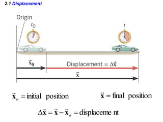
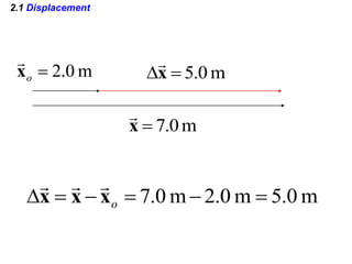
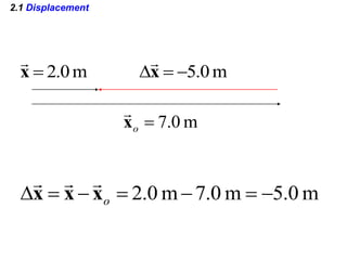
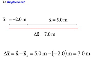
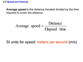
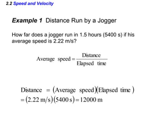
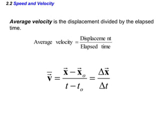
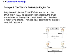
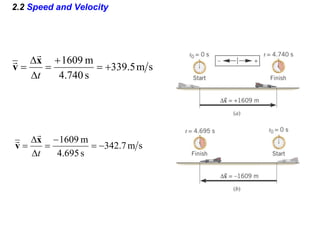
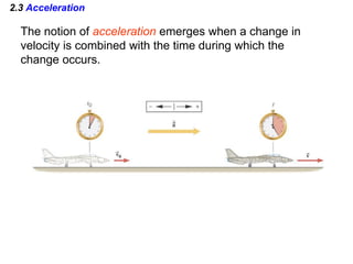
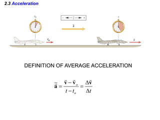
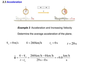
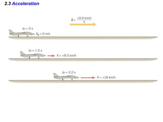
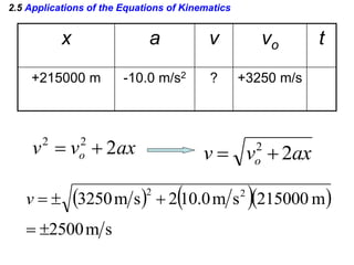
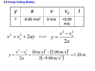
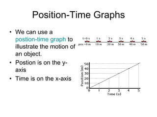
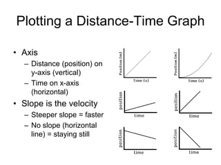
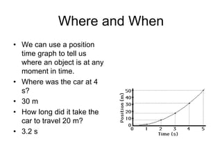
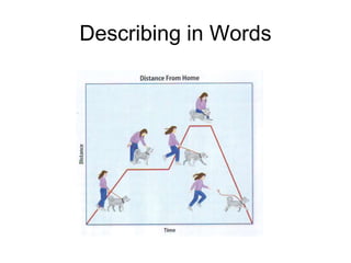
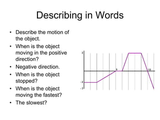
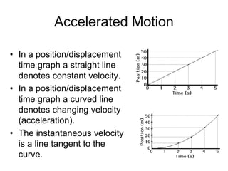
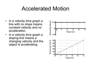
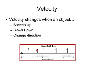
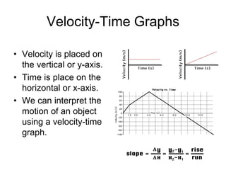
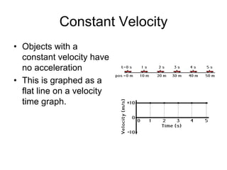
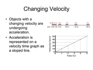
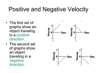
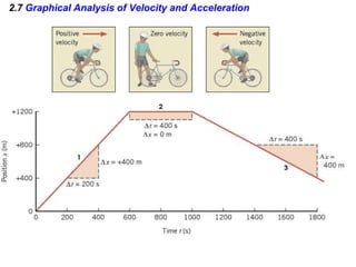
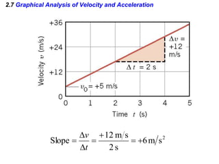
Kinematics deals with concepts of motion like displacement, velocity, and acceleration. Dynamics deals with forces that cause motion. Together they form the branch of mechanics. Displacement is defined as the difference between the final and initial positions. Speed is the distance traveled divided by time. Velocity is displacement divided by time. Acceleration is the rate of change of velocity with respect to time. Equations relate the kinematic variables of displacement, velocity, acceleration, time, and initial velocity. Position-time and velocity-time graphs provide a visual representation of motion and can be analyzed to determine properties like speed, direction of motion, and periods of acceleration.

1. Kinematics in One Dimension
Chapter 2

2. Kinematics deals with the concepts that
are needed to describe motion.
Dynamics deals with the effect that forces
have on motion.
Together, kinematics and dynamics form
the branch of physics known as Mechanics.

3. 2.1 Displacement
position
initial

o
x

position
final

x

nt
displaceme



 o
x
x
x




4. 2.1 Displacement
m
0
.
2

o
x

m
0
.
7

x

m
0
.
5

x

m
0
.
5
m
2.0
m
7.0 




 o
x
x
x




5. 2.1 Displacement
m
0
.
2

x

m
0
.
7

o
x

m
0
.
5


x

m
0
.
5
m
7.0
m
2.0 





 o
x
x
x




6. 2.1 Displacement
m
0
.
2


o
x

m
0
.
7

x

m
0
.
5

x

  m
0
.
7
m
.0
2
m
5.0 





 o
x
x
x




7. 2.2 Speed and Velocity
Average speed is the distance traveled divided by the time
required to cover the distance.
time
Elapsed
Distance
speed
Average 
SI units for speed: meters per second (m/s)

8. 2.2 Speed and Velocity
Example 1 Distance Run by a Jogger
How far does a jogger run in 1.5 hours (5400 s) if his
average speed is 2.22 m/s?
time
Elapsed
Distance
speed
Average 
  
   m
12000
s
5400
s
m
22
.
2
time
Elapsed
speed
Average
Distance




9. 2.2 Speed and Velocity
Average velocity is the displacement divided by the elapsed
time.
time
Elapsed
nt
Displaceme
velocity
Average 
t
t
t o
o






x
x
x
v





10. 2.2 Speed and Velocity
Example 2 The World’s Fastest Jet-Engine Car
Andy Green in the car ThrustSSC set a world record of
341.1 m/s in 1997. To establish such a record, the driver
makes two runs through the course, one in each direction,
to nullify wind effects. From the data, determine the average
velocity for each run.

11. 2.2 Speed and Velocity
s
m
5
.
339
s
4.740
m
1609







t
x
v


s
m
7
.
342
s
4.695
m
1609







t
x
v



12. 2.3 Acceleration
The notion of acceleration emerges when a change in
velocity is combined with the time during which the
change occurs.

13. 2.3 Acceleration
t
t
t o
o






v
v
v
a




DEFINITION OF AVERAGE ACCELERATION

14. 2.3 Acceleration
Example 3 Acceleration and Increasing Velocity
Determine the average acceleration of the plane.
s
m
0

o
v

h
km
260

v

s
0

o
t s
29

t
s
h
km
0
.
9
s
0
s
29
h
km
0
h
km
260








o
o
t
t
v
v
a




15. 2.3 Acceleration

16. 2.3 Acceleration
Example 3 Acceleration and Decreasing
Velocity
2
s
m
0
.
5
s
9
s
12
s
m
28
s
m
13








o
o
t
t
v
v
a




17. 2.4 Equations of Kinematics for Constant Acceleration
Equations of Kinematics for Constant Acceleration
 t
v
v
x o 
 2
1
2
2
1
at
t
v
x o 

at
v
v o 

ax
v
v o 2
2
2



18. 2.4 Equations of Kinematics for Constant Acceleration
Five kinematic variables:
1. displacement, x
2. acceleration (constant), a
3. final velocity (at time t), v
4. initial velocity, vo
5. elapsed time, t

19. 2.4 Equations of Kinematics for Constant Acceleration
     
m
110
s
0
.
8
s
m
0
.
2
s
0
.
8
s
m
0
.
6
2
2
2
1
2
2
1





 at
t
v
x o

20. 2.4 Equations of Kinematics for Constant Acceleration
Example 6 Catapulting a Jet
Find its displacement.
s
m
0

o
v
??

x
2
s
m
31


a
s
m
62


v

21. 2.4 Equations of Kinematics for Constant Acceleration
   
  m
62
s
m
31
2
s
m
0
s
m
62
2 2
2
2
2
2






a
v
v
x o

22. 2.5 Applications of the Equations of Kinematics
Reasoning Strategy
1. Make a drawing.
2. Decide which directions are to be called positive (+) and
negative (-).
3. Write down the values that are given for any of the five
kinematic variables.
4. Verify that the information contains values for at least three
of the five kinematic variables. Select the appropriate equation.
5. When the motion is divided into segments, remember that
the final velocity of one segment is the initial velocity for the next.
6. Keep in mind that there may be two possible answers to a
kinematics problem.

23. 2.5 Applications of the Equations of Kinematics
Example 8 An Accelerating Spacecraft
A spacecraft is traveling with a velocity of +3250 m/s. Suddenly
the retrorockets are fired, and the spacecraft begins to slow down
with an acceleration whose magnitude is 10.0 m/s2. What is
the velocity of the spacecraft when the displacement of the craft
is +215 km, relative to the point where the retrorockets began
firing?
x a v vo t
+215000 m -10.0 m/s2 ? +3250 m/s

24. 2.5 Applications of the Equations of Kinematics
ax
v
v o 2
2
2


x a v vo t
+215000 m -10.0 m/s2 ? +3250 m/s
ax
v
v o 2
2


    
s
m
2500
m
215000
s
m
0
.
10
2
s
m
3250 2
2





v

25. 2.6 Freely Falling Bodies
In the absence of air resistance, it is found that all bodies
at the same location above the Earth fall vertically with
the same acceleration.
This idealized motion is called free-fall and the acceleration
of a freely falling body is called the acceleration due to
gravity.
2
2
s
ft
2
.
32
or
s
m
80
.
9

g

26. 2.6 Freely Falling Bodies
2
s
m
80
.
9

g

27. 2.6 Freely Falling Bodies
Example 10 A Falling Stone
A stone is dropped from the top of a tall building. After 3.00s
of free fall, what is the displacement y of the stone?

28. 2.6 Freely Falling Bodies
y a v vo t
? -9.80 m/s2 0 m/s 3.00 s

29. 2.6 Freely Falling Bodies
y a v vo t
? -9.80 m/s2 0 m/s 3.00 s
     
m
1
.
44
s
00
.
3
s
m
80
.
9
s
00
.
3
s
m
0
2
2
2
1
2
2
1






 at
t
v
y o

30. 2.6 Freely Falling Bodies
Example 12 How High Does it Go?
The referee tosses the coin up
with an initial speed of 5.00m/s.
In the absence if air resistance,
how high does the coin go above
its point of release?

31. 2.6 Freely Falling Bodies
y a v vo t
? -9.80 m/s2 0 m/s +5.00
m/s

32. 2.6 Freely Falling Bodies
y a v vo t
? -9.80 m/s2 0 m/s +5.00
m/s
ay
v
v o 2
2
2


a
v
v
y o
2
2
2


   
  m
28
.
1
s
m
80
.
9
2
s
m
00
.
5
s
m
0
2 2
2
2
2
2






a
v
v
y o

33. 2.6 Freely Falling Bodies
Conceptual Example 14 Acceleration Versus Velocity
There are three parts to the motion of the coin. On the way
up, the coin has a vector velocity that is directed upward and
has decreasing magnitude. At the top of its path, the coin
momentarily has zero velocity. On the way down, the coin
has downward-pointing velocity with an increasing magnitude.
In the absence of air resistance, does the acceleration of the
coin, like the velocity, change from one part to another?

34. 2.6 Freely Falling Bodies
Conceptual Example 15 Taking Advantage of Symmetry
Does the pellet in part b strike the ground beneath the cliff
with a smaller, greater, or the same speed as the pellet
in part a?

35. Position-Time Graphs
• We can use a
postion-time graph to
illustrate the motion of
an object.
• Postion is on the y-
axis
• Time is on the x-axis

36. Plotting a Distance-Time Graph
• Axis
– Distance (position) on
y-axis (vertical)
– Time on x-axis
(horizontal)
• Slope is the velocity
– Steeper slope = faster
– No slope (horizontal
line) = staying still

37. Where and When
• We can use a position
time graph to tell us
where an object is at any
moment in time.
• Where was the car at 4
s?
• 30 m
• How long did it take the
car to travel 20 m?
• 3.2 s

38. Interpret this graph…

39. Describing in Words

40. Describing in Words
• Describe the motion of
the object.
• When is the object
moving in the positive
direction?
• Negative direction.
• When is the object
stopped?
• When is the object
moving the fastest?
• The slowest?

41. Accelerated Motion
• In a position/displacement
time graph a straight line
denotes constant velocity.
• In a position/displacement
time graph a curved line
denotes changing velocity
(acceleration).
• The instantaneous velocity
is a line tangent to the
curve.

42. Accelerated Motion
• In a velocity time graph a
line with no slope means
constant velocity and no
acceleration.
• In a velocity time graph a
sloping line means a
changing velocity and the
object is accelerating.

43. Velocity
• Velocity changes when an object…
– Speeds Up
– Slows Down
– Change direction

44. Velocity-Time Graphs
• Velocity is placed on
the vertical or y-axis.
• Time is place on the
horizontal or x-axis.
• We can interpret the
motion of an object
using a velocity-time
graph.

45. Constant Velocity
• Objects with a
constant velocity have
no acceleration
• This is graphed as a
flat line on a velocity
time graph.

46. Changing Velocity
• Objects with a
changing velocity are
undergoing
acceleration.
• Acceleration is
represented on a
velocity time graph as
a sloped line.

47. Positive and Negative Velocity
• The first set of
graphs show an
object traveling
in a positive
direction.
• The second set
of graphs show
an object
traveling in a
negative
direction.

48. Speeding Up and Slowing Down
•The graphs on the left represent an object
speeding up.
•The graphs on the right represent an object
that is slowing down.

49. Two Stage Rocket
• Between which
time does the
rocket have the
greatest
acceleration?
• At which point
does the velocity
of the rocket
change.

50. Displacement from a Velocity-Time
Graph
• The shaded region under
a velocity time graph
represents the
displacement of the
object.
• The method used to find
the area under a line on a
velocity-time graph
depends on whether the
section bounded by the
line and the axes is a
rectangle, a triangle

51. 2.7 Graphical Analysis of Velocity and Acceleration
s
m
4
s
2
m
8
Slope 






t
x

52. 2.7 Graphical Analysis of Velocity and Acceleration

53. 2.7 Graphical Analysis of Velocity and Acceleration
2
s
m
6
s
2
s
m
12
Slope 






t
v