1. CHAPTER 1: Macroeconomics – An Introduction
Learning Objectives (LO’s) for Chapter:
LO 1.1 Describe in a broad way the goals of economics and specifically macroeconomics.
LO 1.2 Show how macroeconomics can help you understand concepts that directly impact your
material well-being -- ‘bread and butter’ issues.
LO 1.3 Compare the major macroeconomic downturn that has occurred within your lifetime,
the Great Contraction of 2007-09, with previous ones.
LO 1.4 Identify macroeconomic issues from the perspective of policy-oriented economists.
LO 1.5 Explain several of the tools and structured analyses that macroeconomists engage in.
Chapter Overview
Humans make considerable efforts to maintain and improve their material well-being. We work and
sacrifice so as to ensure that we and our families enjoy, at the very least, certain basics: food, shelter,
clothing, and other safeguards for our survival and our health. If we are more fortunate, our material
well-being extends beyond such basics, as reflected in a wide variety of goods and services that we are
able to purchase. We seek a more comfortable existence, we like to partake of diverse pleasures and
forms of entertainment, we communicate instantly with others around the world, and we travel
extensively. New, labor saving, technology can free us from mundane and physically difficult tasks.
Hopefully, this all of this will help enrich our lives in realms that extend beyond our material
possessions.
As an intellectual discipline, economics provides a way for us to understand this drive to sustain and
improve our material well-being. According to what is perhaps the classic definition, economics is the
study of how humans allocate scarce resources. More explicitly, economics is “(t)he social science that
deals with the production, distribution, and consumption of goods and services and with the theory and
management of economies or economic systems.” 1 This chapter introduces you to economics, and
specifically, macroeconomics.
1
See the link: http://www.answers.com/topic/economics
1

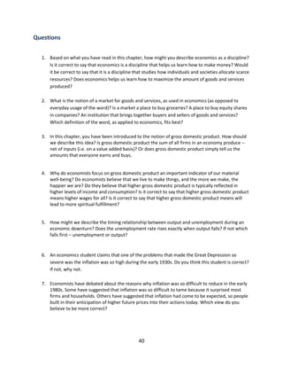
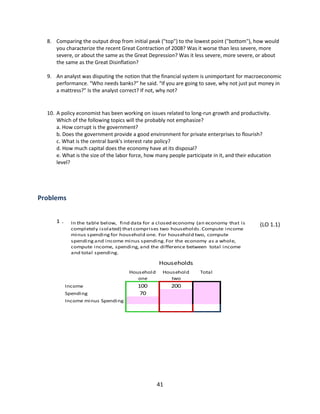
2. 1.1 Economics from the Micro and Macro perspectives
LO 1.1
LO 1.1 Describe in a broad way the goals of economics and specifically macroeconomics.
Economics has been divided into two sub-disciplines: microeconomics and macroeconomics.
Microeconomics focuses on individuals achieve economic goals, either by themselves or through the
organizations that they form. One economic organization that you no doubt have been exposed to is the
family unit or household. [key word: household: a unit of one or more individuals, often a family, that
reside in the same home.] To sustain the people in the household (that is, the family), individuals must o
perform tasks to produce some good or service.
Some of these tasks are take place entirely within the household -- for example, cooking, cleaning, and
caring for children. Outside the home, individuals commonly form and participate in firms:
organizations/enterprises whose main goal is to produce and sell some good or service that is intended
to be traded in a market. [key term: firm: organizations/enterprises whose main goal is to produce and
sell some good or service that is intended to be traded in a market.] [key term: market: an institution
that brings together buyers and sellers of goods and services.]
Individuals provide their work effort to firms for in exchange for some form of compensation – this is
the income that individuals bring back to their households. [key term: work effort: force exerted by
human beings to produce some good or service.] (Key term: income: resources (goods or money) that
people receive, most often as compensation for producing something.] This income enables them to
buy and consume goods that provide them some pleasure or benefit. [key term: consume: the use of
goods that provide some pleasure or benefit.]
Individuals and the firms they work for each typically produces a relatively narrow range of goods and
services – they specialize. For example, some individuals or firms may be especially good at producing,
say, flat-screen televisions. Others without such detailed technical expertise may, for example, produce
extraordinarily good ice cream.
2

3. Figure 1.1
Households and Firms;
Goods and Labor Markets
HH 1
HH 2
LABOR MARKET:
Households supply their
labor to firms; they earn
income as compensation for
their efforts.
Firm 1
Firm 2
HH 3
Firm 3
HH 4
Firm 4
HH 5
Firm 5
HH 6
Firm 6
….
….
GOODS MARKET:
Households purchase and
consume a variety of goods
from firms; each firm
specializes in a limited
number of goods/services.
By contrast, households typically buy a wide range of goods – they do not specialize in consumption.
[key term: consumption: the act of consuming.] As an example, eating ice cream and watching a flatscreen TV are not mutually exclusive activities. In fact, many consumers enjoy eating ice cream while
watching their flat-screen TVs!
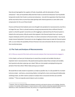
Economists emphasize that markets have a key job to do, namely to bring people together so that they
may trade. Figure 1.1 illustrates this point. In markets for goods and services, households, who demand
goods and/or services, are brought together with firms, which supply these goods or services. A market
may be a physical location – a building or tent in some specific place. But, markets may exist in other
forms, including the digital online markets that have evolved in recent decades. In a labor market
individuals who offer their work effort are brought together with the firms who buy that effort. [key
term: labor market: an institution that brings together buyers of work effort (firms) and sellers of work
effort (individuals from households).] 2
2
In some cases, labor markets exist in physical locations. For example, there may be some place in your
town where manual laborers line up each morning get some sort of work for the day – hauling trash,
gardening, painting, etc. More often, labor markets take on a virtual form – a network of contacts in a
certain profession, for example.
3

4. In this context, one other kind of economic organization needs to be mentioned. In order to conduct
their market transactions in an orderly way, households and firms require a set of rules by which they
conduct their business, and they need to be assured that the rules are enforced. This is one reason that
states or governments arise: to provide an environment for households and firms to function and
prosper!
Individuals and the firms they work for each typically produces a relatively narrow range of goods and
services – they specialize. For example, some individuals or firms may be especially good at producing,
say, flat-screen televisions. Others without such detailed technical expertise may, for example, produce
extraordinarily good ice cream. .
Households buy and consume goods that provide them some pleasure or benefit. [key term: consume:
the use of goods that provide some pleasure or benefit.] The income they receive enables them to do
so. Households typically buy a wide range of goods – they do not specialize in consumption. [key term:
consumption: the act of consuming.] As an example, eating ice cream and watching a flat-screen TV are
not mutually exclusive activities. In fact, many consumers enjoy eating ice cream while watching their
flat-screen TVs!
In a class on microeconomics, we learn that who produces what will reflect comparative advantage.
[key term: comparative advantage: the capacity of an individual or organization to produce a specific
good or service at a lower opportunity cost than others.] There may be some very talented individuals or
firms that are capable of producing both flat-screen TV’s and ice cream better than others. This
individual/firm is said to have an absolute advantage over others in both TVs and ice cream. [Key term:
absolute advantage: the capacity of an individual or organization to produce a good or services more
efficiently than others]. However, if by dedicating all of their efforts to producing TVs, the cost (as
measured in foregone gallons of ice cream) may be less than others in the market. This individual/firm is
said to have a comparative advantage in TV’s; they will let others produce the ice cream.
Microeconomics thus helps us understand how much of a specific good or service is produced, and at
what price. For both demanders and suppliers of a good/service, a key piece of information is the
market price of that good/service. (key term: demander: an individual or organization that wishes to
purchase a good or a service.] [key term: supplier; an individual or organization that is prepared to offer
4

5. a good or a service]. Holding all else equal, an increase in the price of a good/service will encourage
demanders to purchase less but suppliers to produce more. Thus, a key concept in microeconomics is
that the equilibrium price in a market is one where the quantities demanded and supplied of a
good/service are exactly equal. [key term: equilibrium price: the price at which the quantities demanded
and supplied are equal]. 3
If the price of a good/service is (momentarily) below the equilibrium price, the quantity demanded will
exceed the quantity supplied. Producer will be encouraged to produce more in order to meet this extra
demand – but only if the price they receive rises. As this happens, some of the extra demand is choked
off. Ultimately, the price will rise to an equilibrium at which supply equals demand.
From the other direction, if the price is above its equilibrium level, the quantity supplied will exceed the
quantity demanded. Sellers will compete with one another to sell off this excess supply by lowering their
prices. As this happens, more demand is encouraged. This continues until the price reaches an
equilibrium that equates quantities supplied and demanded.
In contrast to the focus of microeconomics on individual markets, macroeconomics puts most of its
emphasis on aggregate concepts and variables – very often, at the level of one or more entire countries.
[key term: aggregate, the combination of many firms and households, most often at the level of one or
more entire countries.] This means that, instead of individual markets (say, ice cream, televisions), we
look at quantities of goods and services produced by the economy as a whole. The most commonly used
aggregate measure of goods and services produced in a country – our output -- is known as gross
domestic product (GDP) – a concept that we will describe more fully in an early chapter of the book.
(Key terms: gross domestic product: the most frequently used measure of a country’s aggregate
output.)
Macroeconomics will focus on measures of an aggregate price level, rather than the prices of one or
several goods. (Key term: aggregate price level: a combined measure of prices of many goods and
services in an economy, as opposed to the price of an individual good or service). A frequently used
measures of the aggregate price level is the consumer price index (CPI). (key term: consumer price
3
If you feel rusty on your supply and demand analysis, don’t worry. We will present an extensive review
in an upcoming chapter.
5

6. index: a combined measure of the prices of the many goods and services that households produce].
These concepts – how we measure them and how they are influenced by economic forces -- will be
discussed at length in this book.
Markets: What job do they do -- and are they doing it?
A question that economists often ask is: “Are markets working correctly?” For example, a
microeconomic analysis that focuses on individual goods/services – the market for ice cream, flat screen
TV’s, and so on – tells us the equilibrium amount of each of these goods/services that will be produced.
If the market is working correctly, supply and demand are will be equated with one another at an
equilibrium price. However, something may prevent the market from doing its job. In some cases,
governments may implement policies that interfere with markets. For example, the government might
impose price controls on the price of ice cream. If the controlled price is less than the equilibrium price,
demand will exceed supply. In this case, we can expect that people will form lines to buy ice cream –
especially on hot days! Microeconomics also provides us with the tools to determine whether markets,
on their own, without guidance from the government, will generate a socially beneficial outcome.
In macroeconomics, we often ask questions related to macroeconomic performance. [key term:
macroeconomic performance: a general term which refers several aspects of the aggregate economy,
including (but not limited to) how much output and prices grow]. How is the economy working? Are we
in good times – or bad? Is there prosperity -- or stagnation? Are the benefits of the economy distributed
broadly or only to a privileged few?
When we ask such questions, we also analyze markets. These include the markets for goods and labor
that we just discussed. But, we will discuss other markets that are important for the economy’s overall
performance. We ask whether markets are working correctly –whether they are doing the job they are
supposed to do. If not, why not? Is there some sort of market friction – some feature of the market that
prevents it from working properly? Has the government imposed policies that are detrimental to market
performance? [key term: market friction: some institution, regulation, or other factor that keeps a
market from working correctly.] We will study episodes when macroeconomic performance was poor –
‘bad times.’ It is precisely at these times that we have to question whether markets function – or are
permitted to function – correctly.
6

7. Saving, Borrowing, and Finance – A Part of Macroeconomics
An important feature of macroeconomic analysis is that, at any point in time, the amount that individual
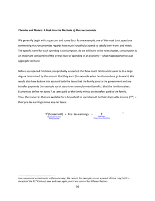
units spend need not equal their income. However, in the aggregate, all income must be spent. To see
what this means, let us consider an imaginary economy that has only two individuals, Claire and Bill. As
shown in Figure 1.2, Claire earns 100 but spends only 90. Because she earns more than she spends we
would say that she saves. [key terms; save: to spend less than one’s income] Bill earns 80 and spends 90.
We say that Bill it dissaves. [key terms; dissave: to spend more than one’s income]
Figure 1.2
Claire saves and Bill
dissaves
Saving and Borrowing
Bill
80
90
-10
(Saves)
Income
Spending
Income minus Spending
Claire
100
90
10
Total
180
180
0
(Borrows)
Let us assume that the Claire-and-Bill economy is located on an island in the middle of the ocean. Its two
resident households have no contact of any kind with anyone else. We would call this a closed
economy. [Key term: closed economy: an economy/country that has no economic relationship with any
other economy / country]. In this case, the sum of all the household balances (earning minus spending)
must be zero. We also see that that, in this simple economy, total spending must equal total income -$180.
We can see that, by saving, Claire has provided Bill with the extra resources that he may spend today. If
Claire had spent all of her income, Bill’s spending today would have been limited to $80. Is this a gift
from Claire to Bill? The answer is “probably not”. If you have previously studied economics, or even if
you haven’t, you may have already learned a phrase that economists enjoy using: “There’s no such thing
as a free lunch.” Instead, Claire is likely providing a $10 loan to Bill, rather than a gift. [Key term: loan:
permission to use resources on a temporary basis, with the expectation that such resources will be
repaid.] A loan carries the expectation of future repayment. That repayment will include the original
7

8. principal of $10 plus some compensation to Claire in return for the use of her resources today. Such
compensation is called an interest payment on the loan. [key term: interest payment; compensation to
someone who has extended a loan].
A loan is one of many financial contracts or agreements that occur in a modern economy. (Key term:
financial contract: an agreement between savers and borrowers which specifies how much and when a
saver is to be repaid.] The story of Claire and Bill is realistic only if they happen to know one another
personally, and Claire wants to save while Bill wants to borrow. In modern economies with many
people, this rarely happens. Instead, disparate savers and borrowers are most frequently brought
through a bank or other financial intermediaries. For example, Claire places her $10 into the bank in the
form of a deposit. Essentially, Claire has provided a loan to the bank – she expects to be able to reclaim
her money at some point in the future. The bank then lends that same $10 out to Bill. In this case, Bill is
expected to repay the $10 more, but to the bank, not to Claire.
One of the important lessons of macroeconomics in recent years is the critical relationship between
macroeconomic performance and the financial system. [key term: financial system: an economy’s
network of banks and other financial intermediaries] A properly functioning financial system can
improve macroeconomic performance. Sometimes, financial systems can cease to function correctly. For
example, if lenders lose confidence that they will be repaid, they may withdraw from the market. When
many lenders do so, a financial crisis may occur. [key term: financial crisis: a situation where confidence
between lenders and borrowers erodes and the financial system ceases to function correctly.] As we will
discuss later in this book, such crises can have substantial and detrimental impacts on an economy’s
performance. And, the relationship in goes in the other direction: poor macroeconomic performance –
for example low levels of output – can drag down the financial system.
1.2 What’s In It for You? Macroeconomics and Your Life
LO 1.2
LO 1.2 Show how macroeconomics can help you understand concepts that directly impact your
material well-being -- ‘bread and butter’ issues.
You may ask whether studying macroeconomics is worth your time – especially since you don’t plan to
become an economist yourself. But, there are reasons why we would expect that a course on
macroeconomics – and perhaps even this specific book -- may be of interest to you. Perhaps the main
8

9. reason is that macroeconomics embraces ideas and concepts that are directly and tangibly related to
your life – including your material well-being.
Gross Domestic Product: A Key Indicator of Our Material Well-Being
As mentioned above, the broadest and most well-known measure of a country’s material well-being is
real gross domestic product (GDP). This is the total economic output of a country -- the total value of all
final goods and services produced in an economy in a period of time. We stress the word ‘final’ since
companies typically purchase inputs (goods and services) to make their product. The difference between
what a firm sells and the inputs it purchases is its value added. [key word: value added; the difference
between what a firm produces and the value of its inputs.] Thus, suppose that a firm sells a shirt for $50,
but that shirt uses $30 worth of cotton. In that case, we would say that the firm’s value added on each
shirt was $20. Thus, GDP is the aggregate variable -- the total of all value added by all firms in an
economy.
The level of GDP is measured in a country’s currency units – the Dollar in the United States is one
example. (Key term: level: the value of a variable at one point in time) We must be sure to use a
measure of measure of GDP that captures as accurately as possible increases or decreases in the
quantity of goods and services that we produce. Economists have developed several measures of real
GDP. [Key term: real GDP; a measure of GDP that permits us to accurately compare values at different
points in time.] Such measures, as we will show in the next chapter, help us know that an increase in
GDP truly reflects an increase in the quantity of goods and services that we are producing. A measure of
nominal GDP, rather than real, GDP, may simply reflect the fact that prices are going up – without any
change in the amount we produce. (key term: nominal GDP; a measure of GDP that does not account for
changes in prices.]
So, GDP is a measure of how much we produce – our output. In what sense is the amount that we
produce connected to our well-being? What does this mean for a country’s citizens? As we will discuss
in greater detail in the next chapter, there is a close correspondence between GDP of a country and the
income that its citizens receive. For the most part, income is the compensation that people receive for
producing something. Then when individuals receive additional income, they have more resources
9

10. available to purchase the goods and services that satisfy the needs and wants of themselves and other
members of their households. In a word, households are able to consume more.
Another way to make the concept of GDP less abstract, we might think about the amount that a country
produces relative to the number of people in that country. For this reason, we calculate per-capita real
GDP: real GDP divided by the population. (Key term: per-capita GDP: a country’s GDP divided by its
population.). Note that this tells us the amount of production of goods and services per person that are
produced – on average. Of course, not everyone will enjoy the same level of per-capita
output/income/consumption. Amongst the more fortunate, income per capita will lie above the
average, while income per person will lie below the national average.
An issue that has received increasing media attention in recent years concerns the extent of income
inequality – the gap in income per capita between the richest members of society and the poorest ones.
(Key term: income inequality: the gap in income per capita between the richest members of society and
the poorest ones.). Income inequality is an important issue. We will address it in this book.
Unfortunately, the simple measure of per-capita GDP cannot tell us very much about income inequality
– precisely because it is a simple average – output over number of people.
Even so, we will find that per-capita GDP is an important measure that merits our attention – even if it
can’t tell us about inequality. And, we will gain some additional insights by looking at GDP per capita not
at just one point in time but over a longer span of history. We do this in Figure 1.3, which shows a graph
of the level of per-capita GDP in the US from 1900 through 2012. You should see several things. Perhaps
the most important feature of this graph is that the line moves steadily upward. This means that, on a
per-person basis, the amount goods and services over this period has moved steadily upward.
10

11. Figure 1.3
United States: Real Per Capita GDP
50,000
1
2007-09
Early
00s
45,000
40,000
Real (2005) US Dollars
35,000
0.9
0.8
Early
1990s
Source: Historical
Statistics of the US
0.7
Early
1970s
30,000
Early
1980s
0.6
World War II
1941-45
25,000
0.5
20,000
0.4
Post World War
Period 1946-49
15,000
0.3
Great
Depression
10,000
0.2
5,000
0.1
0
The blue shaded area
shows the period of low
output levels known as
the Great Depression.
Output declined from
1929 to 1933, and only
gradually recuperated
thereafter.
0
The yellow
shaded
area shows
that output
rebounded
as the US
mobilized
for World
War II.
Just after
World War II,
output fell
back
somewhat.
The National
Bureau of
Economic
Research
includes two
recessions
during this
period.
The early 1970s
were a time of
great political
uncertainty. During
this time, energy
prices rose
considerably, as a
result of an
embargo by oilproducing
countries.
By the late 1970s, the
growth rate of the
general price level –
inflation – had risen
to all time highs. As a
remedy, the central
bank of the US
(Federal Reserve)
cooled the economy
down by raising
interest rates. This
was the Great
Disinflation
11
A relatively short
and mild
downturn in the
early 1990s is
generally
attributed to
restrictive
policies by the
Federal Reserve;
the period
partially
coincided with
the first Gulf
War.
The downturn in the
early 2000s coincided
with the end of the
first internet or
“dot.com” boom.
The Great
Contraction, which
began in 2007, was
the most severe
downturn since the
Great Depression.
Housing markets
played an important
role in this episode.

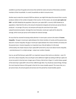
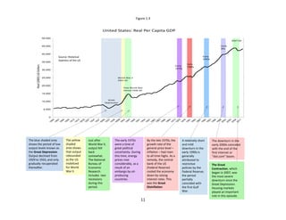
12. This has meant that, on a per-person basis, we have steadily increased the amount that we produce and
that we earn over the past 112 years. That is, over the past century, there has been a substantial
increase in our material well-being. In many ways, this has meant a better life for all. Before you opened
this book, you probably knew that we now enjoy substantially higher levels of health and sanitation than
we did in 1900. 4 Basic items like food and clothing are now more abundant than in 1900. For most, the
work that we do now involves much less physical stress and fewer injuries. And, we now have options
for travel and entertainment that were unimaginable in 1900.
WHERE DID WE GET THOSE NUMBERS (algebra only): Calculating Growth
Rates: We can express the increase in per capita GDP as a number. The
Baseline
alt(i)
alt(ii)
Where did 13260 get those
we
13525
13931
numbers? 2.4
3
2.9
Output
Inflation
Interest Rate
4.5
4.7
4.6
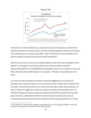
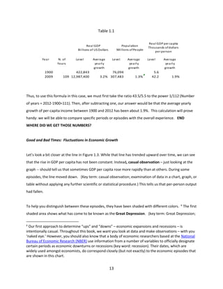
calculations are summarized in Table 1.1. Note that, at the last point of our
data, in 2009, we produced about $42 Thousand per person. At the start of our data, in 1900, we
produced about $5.6 thousand per person. Hence, when we do a division 43.3/5.6, we obtain a result of
7.79. That, in 2009, the US produced almost 8 times on a per-person basis than it did in 1900.
Throughout this book we will be making calculations like this and expressing them in terms of growth
rates that are expressed in percent. For any variable X, the growth rate will be calculated as
%ΔX = XLATER / XEARLIER -1
(
1
.
Hence, in percent (%) terms, per capita income has grown by over 679% (43.3/5.6-1 is about equal to
6.79). This growth has occurred over a period of 112 years (2012-1900). Thus, we can how to calculate
1
the growth rate on an average yearly basis: 5
)
%ΔX(Yearly average)=[(XLATER /XEARLIER )1/N.of Years ]-1
(
1
.
2
4
As one example, we now take for granted that our houses will have indoor plumbing. This convenience
)
was developed during the mid-1800s, but did not become universal in the US until well into the 20th
Century!
5
You might be tempted to simply divide 660 percent by 112. However, you would not get a correct
answer since growth rates are compounded over time.
12

13. Table 1.1
Calculating Growth
Rates
Popul ation
Mi l lions of People
Rea l GDP
Bi l lions of US Dollars
Yea r
1900
2009
N. of
Yea rs
Level
422,843
109 12,987,400
Avera ge
yea rl y
growth
Level
76,094
3.2% 307,483
Avera ge
yea rl y
growth
1.3%
Rea l GDP per ca pita
Thousands of dollars
per person
Level
5.6
42.2
Avera ge
yea rl y
growth
1.9%
Thus, to use this formula in this case, we must first take the ratio 43.5/5.5 to the power 1/112 (Number
of years = 2012-1900=111). Then, after subtracting one, our answer would be that the average yearly
growth of per-capita income between 1900 and 2012 has been about 1.9%. This calculation will prove
handy: we will be able to compare specific periods or episodes with the overall experience. END
WHERE DID WE GET THOSE NUMBERS?
Good and Bad Times: Fluctuations in Economic Growth
Let’s look a bit closer at the line in Figure 1.3. While that line has trended upward over time, we can see
that the rise in GDP per capita has not been constant. Instead, casual observation – just looking at the
graph -- should tell us that sometimes GDP per capita rose more rapidly than at others. During some
episodes, the line moved down. (Key term: casual observation; examination of data in a chart, graph, or
table without applying any further scientific or statistical procedure.) This tells us that per-person output
had fallen.
To help you distinguish between these episodes, they have been shaded with different colors. 6 The first
shaded area shows what has come to be known as the Great Depression. (key term: Great Depression;
6
Our first approach to determine “ups” and “downs” – economic expansions and recessions – is
intentionally casual. Throughout this book, we want you look at data and make observations – with you
‘naked eye.’ However, you should also know that a body of economic researchers based at the National
Bureau of Economic Research (NBER) use information from a number of variables to officially designate
certain periods as economic downturns or recessions (key word: recession). Their dates, which are
widely used amongst economists, do correspond closely (but not exactly) to the economic episodes that
are shown in this chart.
13

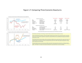
14. a period of economic stagnation that began in 1929 and extended through most of the 1930s.) This was
a period of economic stagnation that began in 1929 and extended through most of the 1930s, with percapita GDP bottoming out in 1933. The term ‘depression’ is often used in geology to denote a valley,
canyon, or dry lakebed. Hence, the term ’depression’ It is an appropriate metaphor for economics: over
the years 1930-34, GDP per capita is 18% lower than it was during the previous 5 year period (1925-29).
From its bottom in 1933, output increased only gradually – until 1941, when the US entered World War
II. At that time, the federal government coordinated efforts to increase production related to the war,
which lasted until 1945. Then, in 1946, just after the armistice, as the US wound down its wartime
efforts, real per-capital GDP again dropped by -- 11% in one year alone.
After this, and into the decades of the 1950s and 60s, the nation enjoyed a period when output grew
more steadily than in previous years. However, the 1970s brought in a period of great political and
economic uncertainty. An embargo by major petroleum exporters (the Organization of Petroleum
Exporting Countries, or OPEC) sent oil prices skyrocketing in 1973 and again in 1979. Civil unrest was
brought on by the Vietnam War. For the first time, a sitting US President, Richard M. Nixon, was forced
to resign as a result of misdeeds in office. Again, at the end of the 1970s and during the early 1980s,
GDP per-capita stagnated; oil prices surged again, and world economies struggled to defeat inflation – a
rise in the price level that continues over time. [key term: inflation; a rise in the price level that
continues over time. ] We call this period during the early 1980s the Great Disinflation. [key term: Great
Disinflation; a period during the late 1970s and early 1980s when inflation, which had been high in
previous years, was brought down.]
The slowdown of 1990-91 (associated with the first Gulf War), and in 2000-01 (associated with the burst
of the “Dot-com” bubble) are also evident. But, most readers of this book are probably more directly
familiar with the economic slowdown that began in 2007 and the meltdown – both financial and
economic – that took place in 2008-09. We will discuss this most recent episode, which we call the Great
Contraction, in the next section of this chapter. [key term: Great Contraction: the fall in economic
activity, associated with a financial crisis, that began in late 2007 and continued through 2009.]
14

15. Figure 1.4
United States: GDP and
Unemployment
a. United States: Real Per Capita GDP
50,000
1
2007-09
Early
00s
45,000
0.9
40,000
0.8
Early
1990s
Constant (2005) US Dollars
35,000
0.7
30,000
25,000
20,000
Early
1980s
Early
1970s
0.6
0.5
World War II
1941-45
Great
Depression
0.4
Post World War
Period 1946-49
15,000
0.3
10,000
0.2
5,000
0.1
0
0
Source: Historical Statistics of the US, Colonial Times to the Present
b. United States: Unemployment Rate
Unemployed/Civilian Labor Force
25
1
2007-09
0.9
Early
00s
20
0.8
Early
1990s
0.7
Early
1970s
In Percent
15
Early
1980s
World War II
1941-45
0.6
0.5
10
0.4
0.3
Post World War
Period 1946-49
5
0.2
Great Depression
0.1
0
0
Source: (1900-46): Historical Statistics of the US, Colonial Times to the Present; Thereafter: Bureau of Labor Statistics
15

16. Employment and Unemployment: Will I Get A Job?
It should not surprise you that a growing economy will generate more job opportunities than a stagnant
one. Businesses that produce more and sell more will typically employ more people. Thus, your personal
opportunities are most likely tied to the economic well-being of the country. When you leave school,
you will probably join the labor force – individuals above 16 years who are working or want to work.
[key term: labor force: individuals above 16 years who are working or want to work.] If you get a job,
you will be counted among individuals who are employed ; until you do so – and it you will most likely
have to look – you will be among the unemployed. [key term: employed: in the labor force currently in a
job.] [key term: unemployed: in the labor force, but without a job – but looking for one.]
The percentage of the labor force that is looking for a job but do not have one is called the
unemployment rate . [key term: unemployment rate: the fraction of the labor force that is currently
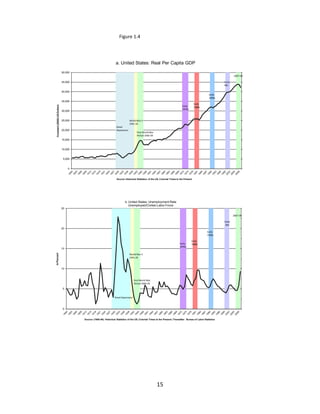
unemployed.] This number for the US is shown from 1900-2009 in Figure 1.4.b (bottom panel) in
percent. GDP per capita for the corresponding period is shown in Figure 1.4.a. (top panel). We can see
how unemployment surged during Great Depression, reaching 23% in 1932. After the Great Depression,
we see episodes where the unemployment rate surged, although not as severely. We can see that
episodes of higher unemployment coincide, for the most part, with the economic downturns that we
introduced in the previous figure.
You may be tempted to think about such changes in the unemployment rate in terms of supply and
demand – concepts which you may be already familiar with. If so, your intuition would be, to a large
extent, correct. During good times, firms demand more labor. When economic activity slows down, they
demand less. Hence in some sense, we might think of unemployment as simply the difference between
labor supply and labor demand.
However, the chart tells us that we have to be careful about the timing. The unemployment rate
typically peaks after the most severe part of the slowdown – just when the economy is beginning to
recover. Why might this happen? When the economy first slows down, employers may be reluctant to
lay off workers – especially their most valued ones. Then, as the slowdown gets under way, some
employers find that they cannot fund their payroll, so they lay off some employees. Then, while an
economic recovery is in a tentative stage, employers may reluctant to take on long term commitments
16

17. when they rehire, and some hire only on a temporary basis. However, when entrepreneurs are more
confident about the economy’s future, hiring occurs more rapidly and the unemployment rate falls.
In this book, we will devote some time to studying labor markets. We will find that the tools of supply
and demand analysis are critical to understand the relationship between output and unemployment. At
the same time, we will find that labor markets have some features not found in other markets. For this
reason, we will need to adapt our supply and demand tools to capture the realities of labor markets.
However, we will find that main job of a labor market is to bring together employers and employees.
Sometimes, labor markets do not do this job well; sometimes there are policies that prevent the labor
market from doing this job well. When this happens, the result that we often see is unemployment that
is higher and longer than need be. As we see below, the Great Depression provides an important, if
tragic, case study where labor markets did not (or were not permitted) to function well. For this reason,
unemployment remained high during the Great Depression – for a considerable period of time.
How much does it cost to live? The Consumer Price Index and Inflation
Nearly everyone is concerned with the cost-of-living. Households can suffer when the prices of key
goods and services they buy rise – if their income does not keep up. Most countries measure the cost of
living by constructing a consumer price index (CPI).
To do so, economists first determine the bundle of goods and services that households typically
purchase in a period of time – food, clothing, housing, domestic services, transportation (including gas,
oil, and upkeep on the family car), entertainment, and so on.
7
The prices are combined into a price
index that attempts to reflect what an “average” or “typical” consumer purchases. [key term: price
index; a combination of several prices that is used to measure the aggregate price level.] The CPI is
often reported in terms of its growth rate in percent over some previous period. This is a measure of
the inflation rate. [key term: inflation rate; the percent growth of prices over the previous period; used
interchangeably with ‘inflation.’] So, if we say that “The Inflation rate is 5% per year,” or equivalently,
“Inflation is 5% per year,” we mean that the CPI is 5% higher today than it was one year ago.
7
In the United States, the CPI is constructed by the Bureau of Labor Statistics (BLS).
http://www.bls.gov/cpi/
17

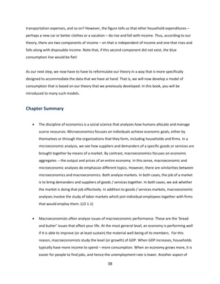
18. Figure 1.5 shows inflation for the US since 1947. We can see that (headline) CPI inflation was high and
volatile in the initial years – just after World War II had ended. During the early 1960s, both inflation
rates were low – less than 2% per year. Then, inflation creeps up – first spiking at just over 6% around
1969 and then spiking twice: first at about 12% per year in 1974 and then at over 16% in 1980.
Figure 1.5
US: CPI Inflation
In percent per year
16
14
12
In Percent year-over-year
10
Headline
8
6
4
2
0
1948
1953
1958
1963
1968
1973
1978
1983
1988
1993
1998
2003
2008
2013
-2
Source: US Bureau of
Labor Statistics
-4
This graph suggests to us in another way why the 1970s were considered a period of economic
turbulence. Not only was inflation high, it was also less predictable than previously. This made it more
difficult for households and businesses to make plans. The graph also shows how inflation came down
during 1980s and 1990s. In this book, we will discuss several explanations as to why this happened. We
can also see that during late 2008 and 2009 inflation became negative. The overall price level (including
both food and energy) dropped by about 2%. From the outset of the financial crisis in 2008, policy
makers were worried about a protracted fall in consumer prices – a deflation. [key term: deflation: a
continued fall in the price level; minus one times inflation.] The concern is that, under a deflation, when
people expect prices to drop in the future they may delay their purchases until they can benefit even
more from lower prices. Hence, the danger of deflation lies in the possibility that demand and prices
might pull one another down in a vicious downward spiral.
18

19. It is not possible to talk about inflation without mentioning in institution that exists in most countries: a
central bank. [key term: central bank: a public, or partially-public institution whose main responsibilities
include the maintenance of a stable rate of inflation]. Central banks are typically part of the
government. However, in most countries, the central bank has been granted some independence from
day-to-day political affairs. In the US, the central bank is called the Federal Reserve (or more commonly,
the ‘Fed’.) 8 Central banks issue a financial instrument that we use every day to conduct our
transactions: money. (key term: money: a financial instrument used for day-to-day transactions and that
performs several other functions.) In this book we will learn how the policies of the central bank,
including how much money they issue, will have an impact on the inflation rate.
How Wealthy Are We? Stock Market and House Values
The assets that people hold, in addition to the income that they earn from their employment, represent
resources that are available for them to spend and enjoy. [key term: asset; a resource held by some
person, household, firm, or country that confers and economic benefit.] There many different kinds of
assets – too many to discuss here. However, there are two kinds of assets in particular that you are
probably familiar with and whose value can be substantially impacted by macroeconomic events.
First, many households own equity shares. [key term: equity share; a financial instrument that grants
someone the right to some portion of a firm’s earnings; equity shares are commonly known as “stocks”.]
They may have purchased stocks in a direct manner, buying and selling online or through a stock broker.
Or, they may hold equity shares indirectly, through a mutual fund or a retirement plan. - By owning
equity shares in a firm, households can participate in the fortunes of that firm – good or bad. When a
firms profits increase (or are expected to increase in the future), the household benefit because the
equity share price (or stock price) rises. When a firm’s profits decrease (or are expected to decrease in
the future), the household loses because the equity share price (or stock price) falls.
8
Several countries may join a monetary union. [key term: monetary union; multiple political units that
use the same money]. In this case, they will be served by one central bank. For example, members of the
Euro area (17 European countries in all) are served by the European Central Bank (ECB). In most
countries or monetary unions, the central bank operates under a mandate or charter whose primary
goal is to make sure that the aggregate price level remains firmly under control . (key terms; mandate,
charter). However, in most countries, central banks will have other, broader goals that are related to
improving the country’s economic performance.
19

20. Equity shares are traded on a country’s stock market (or stock exchange). [key term: stock market: an
institution that brings together buyers and sellers of equity shares; the most well-known example of a
stock market in the United States is the New York Stock Exchange.] Equity share prices of many
companies are put together and published daily as stock price indices. (key term: stock price indices).
You may already be familiar with the idea of a stock market, including the widely used indices such as
the Dow Jones Industrial Average (DJIA), the Standard and Poor’s 500 Index (S and P 500), and the
NASDAQ Composite. 9
Stock price indices thus reflect the sales and income prospects of many firms in an economy. In this
sense, these indices – often referred to in the popular press and the “stock market” can serve as an
important barometer of broader the macroeconomic picture. When things are going well in the
economy, firms will sell more goods and services. This is precisely when more people will want to own
equity shares in firms, since their goal is to participate in firms’ good times. Accordingly, prices of equity
shares rise. In the other direction, when things are going poorly in the economy, firms sell less. In this
instance, people will sell their equity shares, and their prices fall.
But, there is another linkage between stock markets and the economy. As we will discuss later in this
book households who are fortunate enough to hold equity shares when their value rises have essentially
received some extra income – so they spend more. In the other direction, when equity share prices fall,
these households tend to spend less.
The other asset of importance to families is real estate – for example, their house. For many individuals
In many case, a house is an individual’s main asset. While people live in their homes, most recognize
that, if they needed to, they could sell their house for cash. They may see the connection: higher house
value, more cash. This line of thought, of course, is incomplete: it ignores where else they might live if
they did sell their house.
9
The acronym NASDAQ originally stood for National Association of Securities Dealers Automated
Quotations).
20

21. Figure 1.6: Macroeconomics and Asset Prices:
The Recent Experience in the United States
a. United States: Real Gross Domestic Product
Billions of Real (2005) Dollars
14000
Onset of great contraction
13800
13600
13400
13200
13000
12800
12600
Sources: Bureau of
Economic Analysis/Haver
Analytics.
12400
12200
The blue line in figure a (top panel) shows real gross domestic product in the
United States in recent years. Most economists agree that the recent
economic downturn (which we have named the “Great Contraction”) began in
the last months of 2007. Its most severe period occurred between late 2008
(where the blue line falls most sharply) through the middle of 2009. Since
then, real GDP has recovered. However, in some ways, the economy is not
performing as well as many feel it should. As we have noted, unemployment
has not fully recuperated. For many, it is more difficult to get a job than before
the downturn.
12000
b. United States: Real Equity Prices
750
700
Index
650
600
550
500
450
Sources: Standard and
Poor's/Bureau of Economic
Analysis/Haver Analytics.
400
350
300
c. United States: Real House Prices
100
Index
90
80
70
60
Sources: Standard and
50 Poor's/Case - Shiller /Bureau
of Economic Analysis/Haver
40 Analytics.
The green line in figure b (middle panel) shows an index of equity share prices
for the United States, adjusted for changes in the cost of living. An upward
movement of the line typically signals an improvement in firms’ prospects. For
people who own equity shares (either directly or indirectly) a rise in the line
represents an increase in resources available for them to spend –more
household consumption. Equity prices reached a peak and began to fall just
before the onset of the economic downturn. Then, the stock market
plummeted severely and in anticipation of the drop in output. Many
households reacted by cutting back their spending. Since the early months of
2009, equity prices have recovered – but only gradually and unevenly.
The red line in figure c (bottom panel) shows an index of house prices for the
United States. Again, the index is adjusted for changes in the cost of living. An
upward movement of the line tells us that, on average, the sale price of houses
has increased. For over a decade, houses prices had been increasing. Greater
availability of mortgage lending encouraged many new houses to be built – too
many for the market to absorb. By 2005, house prices had topped out and
began to fall. For many families, the house is the principal asset. If their house
value declines sharply they will likely cut back their spending – especially if the
house value falls below the value of the mortgage, leaving the homeowner
“under water.” Since the crisis, most house values have not returned their
previous values.
Real equity price index: Standard and Poor’s 500 deflated by CPI.
Real house price index: Case Shiller deflated by CPI.
21

22. Most individuals/families do not have the resources to purchase a home outright. Instead most rely on
borrowed funds in the form of a long-term mortgage loan. [key term: mortgage; a long term loan that is
extended, most generally for the purchase of a house.]. As is the case with other loan, recipients of a
mortgage are expected to repay their lender a specified amount on specified schedule. In this case the
value of the house can take on more importance. Home owners with mortgages are (or should be)
aware of whether their house value exceeds their loan value. No one wants to be “under water” – a
situation where the loan is worth more than the house itself!
You were probably familiar with these assets before you opened this book. Your personal situation, or
that of your family, may have been impacted by recent shifts in the stock market and the real estate
market. What you may not be aware of are the many linkages between assets like equities and real
estate and broader macroeconomic concepts. We will discuss such linkages in this book. To begin,
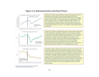
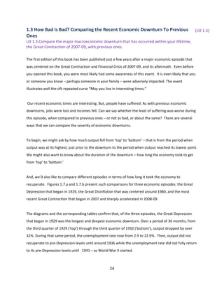
Figures 1.6.a and 1.6.b illustrate some of these linkages during recent years in the United States. In
Figure 1.6.a (top panel), the blue line shows real gross domestic product in the United States in recent
years.
As discussed previously, the recent economic downturn (which we have named the “Great Contraction”)
began in the latter part of 2007. Its most severe phase began in late 2008 (where the blue line falls most
sharply) and lasted through the middle of 2009, when output bottomed out and began to recover. Even
though real GDP has returned to its pre-downturn values, some aspects of macroeconomic performance
remain subpar. Perhaps the key example is unemployment, which had not recuperated even four years
after the downturn ended. For many, getting a job is problematic – much more than before the
downturn.
In Figure 1.6.b (middle panel), the green line shows a well-known index of equity share prices for the
United States, the Standard and Poor’s 500 index. The index is said to be a “real” index because adjusted
for changes in the cost of living. You will learn how to make such an adjustment in this book. An upward
movement of the line typically signals an improvement in firms’ prospects, while a downward
movement signals a deterioration. For people who own equity shares (either directly or indirectly) a rise
in the line represents an increase in resources available for them to spend – more household
consumption; a downward movement means fewer such resources.
22

23. Equity prices reached their peak and began to fall just before the onset of the economic downturn, at
first gradually but then more severely. In the fall of 2008, as a major financial institution (Lehman
Brothers) failed, and people lost confidence in both the financial system and the economy, they sold off
their equity shares, causing equity share prices to plummet even more sharply. In this sense, equity
share prices served as an important barometer of the broader macroeconomic picture: the stock market
was signaling that sales and output were going to fall. However, most economists also believe that there
is a linkage between the stock market and the economy that goes in the other direction: many
households reacted by cutting back their spending. Since the early months of 2009, along with output,
equity prices have since recovered – but only gradually and unevenly. This recovery of equity share
prices has been a factor that has helped to boost spending by households.
In Figure 1.6.c (bottom panel), the red line shows an index of house prices for the United States. As with
the equity price index, this one is also is adjusted for changes in the cost of living. An upward movement
of the line tells us that, on average, the sale price of houses has increased. Such increases had been
occurring steadily in the United States for much of the previous decade. For several reasons, including
easier standards for mortgage lending, many more new homes were built. Ultimately, there were more
houses than the market could absorb without a fall in house prices. By 2005, house prices had reached
an all-time high. We will touch upon the housing market in greater detail later in this book. For many
families, a house, rather than equity shares or other financial instruments, serves as their principal asset.
A decline in the value of their house can have substantial impacts on their wealth and spending. This is
especially true if the value of the house falls below the value of their mortgage loan, as happened to
many families during the economic downturn. Households who owe more than they own are said to be
“under water.” In the years since 2009, house prices have stopped falling so dramatically, but they still
remain substantially below their 2005 peak.
23

24. 1.3 How Bad is Bad? Comparing the Recent Economic Downturn To Previous
Ones
(LO 1.3)
LO 1.3 Compare the major macroeconomic downturn that has occurred within your lifetime,
the Great Contraction of 2007-09, with previous ones.
The first edition of this book has been published just a few years after a major economic episode that
was centered on the Great Contraction and Financial Crisis of 2007-09, and its aftermath. Even before
you opened this book, you were most likely had some awareness of this event. It is even likely that you
or someone you know – perhaps someone in your family – were adversely impacted. The event
illustrates well the oft-repeated curse “May you live in interesting times.”
Our recent economic times are interesting. But, people have suffered. As with previous economic
downturns, jobs were lost and incomes fell. Can we say whether the level of suffering was worse during
this episode, when compared to previous ones – or not as bad, or about the same? There are several
ways that we can compare the severity of economic downturns.
To begin, we might ask by how much output fell from ‘top’ to ‘bottom’ – that is from the period when
output was at its highest, just prior to the downturn to the period when output reached its lowest point.
We might also want to know about the duration of the downturn – how long the economy took to get
from ‘top’ to ‘bottom.’
And, we’d also like to compare different episodes in terms of how long it took the economy to
recuperate. Figures 1.7.a and 1.7.b present such comparisons for three economic episodes: the Great
Depression that began in 1929, the Great Disinflation that was centered around 1980, and the most
recent Great Contraction that began in 2007 and sharply accelerated in 2008-09.
The diagrams and the corresponding tables confirm that, of the three episodes, the Great Depression
that began in 1929 was the longest and deepest economic downturn. Over a period of 36 months, from
the third quarter of 1929 ('top') through the third quarter of 1932 ('bottom'), output dropped by over
32%. During that same period, the unemployment rate rose from 2.9 to 22.9%. Then, output did not
recuperate to pre-Depression levels until around 1936 while the unemployment rate did not fully return
to its pre-Depression levels until 1941 – as World War II started.
24

25. Figure 1.7: Comparing Three Economic Downturns
The Recent Experience in the United States
a. Comparison of Great Depression (1929-33) with Great Contraction (2007-09)
10.0
Comparison of output levels
Top to bottom:
Output drop of 4.7%,
21 months.
5.0
0.0
-5.0
Great Contraction 2007 - 09
-10.0
Great Depression 1929 - 33
-15.0
'Top'
'Bottom'
'Top to bottom'
Duration
Recuperation Date
Duration
Pre-downturn peak
Lowest point
Fall in output, percent
Number of Months
Return of economy
Number of Months
Great Depression
Great Contraction
Q3-1929
Q3-1932
32.6%
36
1936
(approx) 48
Great Disinflation
"double dip"
Q1 1980
Q3 80 / Q1 82
2.2%/0.8%
…
Q1 1983
…
2.9
22.9
20.0
1941
(approx) 144
6.3
10.4
4.1
Q3 1987
90
4.7
9.8
5.2
Not yet
Unknown -- 72 or more
Q3-2007
Q2-2009
4.7%
21
Q4-2011
30
-20.0
Comparison of unemployment rates
Top to bottom:
Output drop of 32%,
48 months.
-25.0
-30.0
-35.0
-40.0
-10
-5
0
5
10
15
20
25
b. Comparison of Great Disinflaton (1980-82) with Great Contraction (2007-09)
10.0
'Top'
'Bottom'
'Top to bottom'
Recuperation Date
Duration
Pre-downturn unemployment
Worst unemployment
Rise in unemployment
Return of unemployment to pre-downturn level
Number of Months
Sources: Statistical Abstract, Bureau of Economic Analysis, Bureau of Labor Statistics, Haver Analytics
The table above and the figures to the left help us compare the depth and duration of economic downturns in the US. '
8.0
"Double dip"
Output drops
6.0
Great Contraction 2007 - 09
Great Disinflation 1980 - 82
4.0
2.0
0.0
The more recent Great Contraction that began in 2007 and accelerated in 2008 -09 was also a severe downturn But, it was much less severe than
the Great Depression. Over a period of 21 months, from the third quarter of 2007(‘top') through the third quarter of 2009 ('bottom'), output
dropped by under 5%. During that same period, the unemployment rate rose from 4.7% to 9.8%. While output has recuperated to its previous
levels, unemployment has remained high.
-2.0
Top to bottom:
Output drop of 4.7%,
21 months.
-4.0
-6.0
-8.0
-10.0
-10
-5
0
5
10
Clearly, the Great Depression that began in 1929 was the longest and deepest economic downturn. Over a period of 36 months, from the third
quarter of 1929 ('top') through the third quarter of 1932 ('bottom'), output dropped by over 32%. During that same period, the unemployment
rate rose from 2.9 to 22.9%. Then, output did not recuperate to pre-Depression levels until around 1936 while the unemployment rate did not
fully recuperate until 1941.
15
20
25
The Great Disinflation, which occured during the early 1980s involved multiple output drops which we ometime call a "double dip recession.".
Overall, this episode was shorter and less severe than the Great Contraction. The unemployment rate reached a higher peak than in the recent
episode -- 10%. However, more people have remained unemployed for a longer period of time in the more recent episode.
25

26. The more recent Great Contraction that began in 2007 and accelerated in 2008 -09 was also a severe
downturn But, it was much less severe than the Great Depression. Over a period of 21 months, from the
third quarter of 2007(‘top') through the third quarter of 2009 ('bottom'), output dropped by under 5%.
During that same period, the unemployment rate rose from 4.7% to 9.8%. By 2011, output recuperated
to its previous levels. However, unemployment has remained stubbornly high. Things still haven’t gotten
back to normal.
The Great Disinflation, which occurred during the early 1980s involved multiple output drops – a socalled "double dip recession" -- is arguably the shortest and least severe of the three episodes. During
this episode, the unemployment rate peaked out at 10% -- a level higher than that of the more recent
Great Contraction. However the duration of high unemployment has been more severe during this
recent episode: people have remained unemployed for a longer period of time.
What’s Your View: How did the Great Contraction affect you?
You, members of your family, and your friends all most likely were personally
affected by the financial crisis and the Great Contraction. Do you know people
What’s Your View?
How did the Great
Contraction Affect
You?
who lost their jobs? Did they find a new one, or are they still unemployed?
Or, do you know anyone who was of a more advanced in age and ready to retire – but did not. Perhaps
their financial nest egg was wiped away. Did you or anyone you know lose their house? Were they
forced into bankruptcy? According to the GDP numbers, the country has recovered from the Great
Recession. But, does it feel like we’ve recovered?
What’s your view? In a course like this one, you will often learn more about the material if you are able
to tie it to your own life. The time to begin is now. We invite you to discuss these issues with your
professor and your fellow students. Of course, as you proceed through the course, your opinions may
change. However, you should begin to ask critical questions now. You are invited into the debate – to
take a view! END WHAT’S YOUR VIEW
26

27. 1.4 Looking Through the Eyes of a Policy-Oriented Macroeconomist
LO 1.4
LO 1.4 Identify macroeconomic issues from the perspective of policy-oriented economists.
We’ve just described some “bread and butter” concepts that affect nearly everyone’s lives. However,
macroeconomics (along with other branches of economics) is a scientific discipline. As such,
macroeconomics requires an analytical structure – not just description. The discipline of
macroeconomics comprises a body of theories and hypotheses, many of which are discussed in this
book. Most macroeconomists in academia specialize in formulating and testing such theories with the
aim of disseminating their results amongst their peers, including through publication in refereed
academic journals.
Macroeconomics is also an applied discipline. Today, elected office-holders ignore macroeconomics only
at their peril. And, governments in most countries, including the US, employ substantial numbers of
policy-oriented macroeconomists – people who are typically well-versed in the findings of their
academic colleagues (they often conduct their own original research) but who are also engaged on a
day-to-day basis on making practical assessments and designing policy recommendations. Beyond
national governments, international organizations like the International Monetary Fund (IMF), the
World Bank (WB), and the Organization for Economic Cooperation and Development (OECD) are also
heavily involved with macroeconomics policy from a practical point of view.
Applied macroeconomics touches on many topics, and sometimes topics overlap. At the risk of
simplifying, today’s applied macroeconomist is concerned with five broad issues. For each issue, a
policy-oriented economist might bring results from economic research (including perhaps their own) to
bear on the recent or current circumstances faced by a country or region. Where does the country
stand? Where are the weaknesses or vulnerabilities that the country that a country faces? How would
these weaknesses affect the citizens of the country? What are the policy remedies at hand for a
country’s government or its central bank?
Issue I: Growth and productivity: What determines an economy’s underlying productivity? What
makes an economy grow? Why do some economies grow more rapidly than others? What policies
will help our country grow more?
As we will discuss in later chapters, to produce any output, inputs are required – what economists term
factors of production.[key term: factors of production: goods and services used to produce other goods
27

28. and services]. The three most frequently cited factors are land (T – from the Latin ‘terra’), the labor
force (L) and capital (K). [key term: capital: a factor of production that itself is produced by humans,
often (but not exclusively) refers to the plant equipment held by firms.) Capital is often (but not
exclusively) used to refer to the buildings, machinery, and other goods that firms use to produce their
good or service. To analyze how these three factors are combined to produce output, economists use
yet another simplification of reality – a production function. [key term: production function: a compact
way of describing the process of producing goods and services that economists use in their analysis.] A
larger labor force, with more people going to work, will raise output. Likewise, higher labor quality in the
form of better educated workers with better work habits will also mean higher output. If countries
dedicate more of their resources to increasing the productive capital, output will also increase.
We sometimes find while two different countries that each use similar amounts of land, labor, and
capital but produce very different levels of output. What makes some countries more productive than
others? Empirical research suggests that certain institutions and policies have important impacts on
productivity. The institutional framework in some countries may provide a more favorable environment
for growth. An example: countries with less corrupt governments tend to grow more than their more
corrupt counterparts.
The answers to such questions should help determine what policies are taken. Hopefully, economists,
like doctors, would first wish to ‘do no harm.’ They would hopefully wish to avoid implementing policies
that reduce growth. Beyond that, economists should also hopefully have something to say about the
kinds of policy reforms that would help boost growth.
Issue II: Output and Price Stabilization: Is our country’s output “too high” or “too low” relative to its
normal (or potential) level? What are the implications for inflation? If so, what (if anything) should
policy makers do?
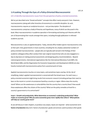
There is a broad consensus that any point in time there is some normal or potential level of output for
an economy. [key term: potential output: the level of output that corresponds to the long-run constraint
implied by the production function, with land, labor, and capital all used a long-run or normal levels.]
Most economists would agree that the potential output corresponds to the long-run constraint implied
by the production function, with land, labor, and capital all used at their long-run or normal levels.
When output is less than its potential, factors of production are used at below-normal levels.
28

29. As we saw for the US, during economic downturns, employment of labor typically falls, and
unemployment rises. Likewise, during such periods, land and capital are used less intensively than
normal. Factories may run fewer shifts, and some may be idled for a time. During such periods, since
demand is weak, inflation can remain subdued.
Conversely, when output more than its potential, factors of production are used at above-normal levels.
During such periods, employment of labor typically rises, and unemployment falls. Existing factories
may run more shifts than normal, and more new plants typically come online. During these periods,
since demand is strong, the inflation rate may rise.
When output is below its potential, expansionary monetary policy (lower interest rates, more money
and credit creation) can be rapidly implemented by a country’s central bank (in the US, this is the
Federal Reserve). Expansionary fiscal policy (cutting taxes, raising expenditures), can also help boost
activity, but such a policy typically suffers delays in implementation. When output is above its potential
level, activity might be reduced either through restrictive monetary policy (higher interest rates, less
lending) or fiscal policy (raising taxes, cutting expenditures).
To what extent, if at all, should policy makers attempt to stabilize the economy? Some would argue that
attempts to ‘fine tune’ the economy can have only a limited effect. Some have even suggested that
policy makers should exclusively dedicate their efforts to increasing productivity, since their efforts at
stabilization will most likely bring few benefits. 10
However, this view may be an extreme one. It may not apply to episodes like the recent crisis and
recession in which a very large shock can cause a severe drop in both economic activity and
employment. In the US and most other countries, governments responded to this shock with
extraordinary measures – measures that we will discuss later in this book.
10
See for example, the 2003 Presidential Lecture for the American Economic Association,
http://home.uchicago.edu/~sogrodow/homepage/paddress03.pdf od Professor Robert Lucas, Nobel
Laureate in Economics.
29

30. Stabilization policy can be also be important is when the economy is overheating – when output
substantially exceeds its potential and inflation is rising. [key term: overheating; a metaphor used to
describe an economy whose output is substantially above potential and, in some cases, whose inflation
rate is rising] Unless the authorities reduce demand, by putting on the policy ‘breaks’ (with monetary
policy typically implemented more quickly than fiscal policy), inflation may rise to undesirable levels and
may even spin out of control.
Issue III: External Balance: Is our country importing too much and/exporting too little (or vice versa)?
Are we living beyond our means and borrowing too much from foreigners?
In recent years, the economy of the United States has become increasingly integrated into the world
economy. We have been selling more to the rest of the world. As Figure 1.8 shows, our exports (sales of
goods and services to the rest of the world) were just under 10% of GDP in 1991. [key term: exports:
sales of goods and services by one country to the rest of the world]. By 2010, after recuperating from
the world downturn, our exports had grown to about 12½% of GDP. Likewise, our imports (purchases of
goods and services from the rest of the world) were just over 10% of GDP in 1991. By 2010, our imports
had grown to about 16% of GDP.
11
[key term: imports: purchases of goods and services by one country
from the rest of the world].
Figure 1.8
United States: Exports and Imports
In percent of GDP
20
15
in percent of GDP
10
Net Exports
5
Exports (Goods+Services)
Imports (Goods+Services)
0
-5
Source: IMF/IFS
-10
In fact, United States’ imports have far outpaced exports. The gap between exports and imports, known
as net exports (or interchangeably the trade balance; net exports = exports minus imports) has become
11
The services include transportation, tourism, insurance, communications, and license fees. How we
compute exports and imports – the balance of payments – is discussed in Chapter _.
30

31. increasingly negative – a trade balance deficit. [key term: net exports: the difference between a
country’s exports and imports; also known as its trade balance]. [key term: trade balance: equivalent to
net exports].
If exports exceed imports, we say that the country is running a trade balance surplus. If we measure
everything accurately there must be a one-to-one linkage between one country’s deficit and a
corresponding surplus for the rest of the world. 12
Many economists have suggested that there are risks associated with the large deficits for the United
States and large corresponding surpluses for China and other countries. Such global imbalances surely
have had impacts in the everyday lives of citizens.[key term: global imbalances: the large deficits of the
United States observed during the 1990s and early 2000s that correspond to large surpluses in other
countries.] In the US, consumers have enjoyed an abundance of imported goods from China (and other
‘emerging markets’ in recent years) -- electronics, clothing, footwear, toys, sporting goods, and so on.
From the Chinese perspective, export-related jobs have helped lift many Chinese workers out of
extreme poverty.
As a country such as the US continues to run external (trade balance) deficits, it accumulates ever more
obligations to the rest of the world – including external debt. [key term: external debt: a country’s
borrowed obligations to the rest of the world.] A country’s external debt cannot grow forever. For this
reason, the global imbalances that we now observe cannot last forever.13 Just as a country’s output will
return to its normal or potential level, its trade balance will also return, from a position of imbalance’ -a deficit or a surplus that is ‘too high’-- to a more balanced position.
12
That is, suppose there are three countries in the world, A, B and C. If country A’s net exports are -5
and country B’s net exports are 2, country C’s net exports must be 3. Thus, the sum of net exports for A
plus B plus C must sum to zero – if measured correctly. In reality, the actual data for the world does not
add up. This situation led some facetiously speculate that the planet Earth is running a deficit with the
planet Mars.
13
Economists have long recognized that the stability of a country’s output level (Issue II) and its external
accounts (Issue III) are parallel issues and cannot be in isolation of one another. This view is associated
with the work of Robert Mundell, a Nobel Prize Winner in Economics (see Mundell, R. , 1962,“The
Appropriate Use of Monetary and Fiscal Policy for External and Internal Stability,” IMF Staff Papers,
March, pp. 70-79.)
31

32. How will these imbalances be resolved? Will the United States be able to repay its debt? Will other
countries, including China, continue to lend to the United States – even if its debt obligations continue
to grow? If the United States’ external debt becomes too high for it to repay, will the country be able to
negotiate some sort of orderly work-out with lenders such as China? Or, in a less-orderly manner will the
United States unilaterally repudiate its debt, potentially causing market participants to lose their
confidence in the United States economy. Will such events bring about an externally-based crisis and
perhaps another Great Depression? [key term: externally-based crisis: a loss of confidence by the rest of
the world in a country’s economic policies or capacity to repay its external debt; such crises can often
lead to severe economic downturns.]
Figure 1.9
United States: Public Debt/GDP
in percent
120.00
Peak of debt ratio after
World War II.
Alternative
scenario by
independent
analyst.
100.00
In percent of GDP
80.00
Data prior to
2012 is historic.
60.00
Official
(CBO)
baseline
scenario
40.00
20.00
0.00
1940
1945
1950
1955
1960
1965
1970
1975
1980
1985
1990
1995
2000
2005
2010
2015
2020
Source: Congressional Budge Office, Long Term Budget Outlook May 2013; alternative
scenario reflects author's calculations. Measure is debt held by the public.
Issue IV: Public Sector Budget Balance: Will our country’s government be able to service its financial
obligations?
In the aftermath of the recent recession, government deficits – the excess of the government’s
expenditures over revenues -- grew dramatically in many countries, including the United States. As GDP
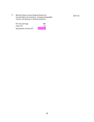
dropped, so also did tax revenue -- a government’s main source of income. [key term: tax revenue (or
taxes); resources that the government collects from households and firms in order to fund its
expenditures.]
32

33. At the same time, in some countries, certain kinds of spending, including social safety net expenditures
designed to help the least advantaged households, including unemployment benefits, also rose during
the downturn. [key term: social safety net expenditures: spending targeted toward helping the least
advantaged households; a prime example is unemployment benefits] In the United States, a newlyelected government under President Barack Obama passed a fiscal stimulus package of temporary
spending increases and tax cuts with the aim of bolstering the aggregate demand for goods and
services. [key term: fiscal stimulus: increases in expenditures or reductions of taxes that the government
makes with the intent of stimulating economic activity during periods of weak output.][key term:
aggregate demand: the demand for all goods and services, in the aggregate.] That package contributed
tangibly to US government debt: it totaled $787 billion dollars (just below 6% of a single year’s GDP).
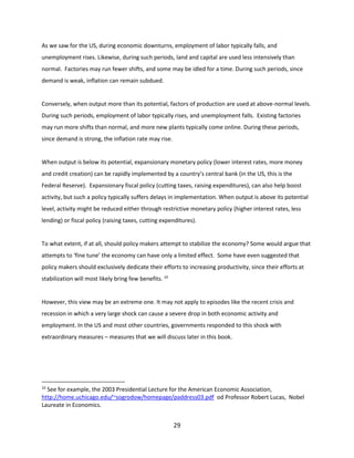
When a government runs a deficit its debt increases. Figure 1.9 shows how US government debt as a
fraction of GDP has evolved since 1940. The chart shows that the government had to borrow
considerably to finance World War II. In 1947, the debt ratio peaked at around 108% of GDP before
gradually falling to about 28% in the early 1970s. [key term: debt ratio: the ratio of government debt –
its accumulated borrowings – to gross domestic product.]
Unlike the other charts shown in this introductory chapter, this one also shows a projection of the debt
ratio – a prediction of where that number may go in the future. [key term: projection: an educated
guess or prediction of what may happen in the future based on specific assumptions.] The Congressional
Budget Office (CBO) of the United States is charged with providing such likely scenarios of prospective
government income, outlays, and government debt. Such forecasts are provided to help the
government plan its policies.
Under a scenario that assumes that current policies remain in place – a baseline scenario -- the debt
ratio is forecast to rise to almost 80% of GDP by 2023 – a figure that has not been seen since early
1950s. [key term: baseline scenario: a projection that shows the most likely outcome, in the opinion of
the experts who make the economic assessment.]
As you might imagine, things might not evolve as the CBO envisages. Things may go worse. The
government may spend more money – say on an unexpected war – or its tax revenues may fall for some
reason. For this reason, analysts often also prepare an alternative scenario that shows what might
33

34. happen under alternative, less favorable circumstances. Under the scenario shown in the chart,
presented by an alternative analysis, the debt grows each year somewhat more than under the baseline.
However, by 2023, the debt will have risen, under this scenario, to over 100% of output – number that
the country has not seen since World War II! [key term: alternative scenario; a projection that shows
the an outcome that is less likely than the baseline scenario but likely enough for people to pay
attention to, in the opinion of experts who make the economic assessment.]
Government debt (in relation to a country’s output) cannot rise forever. If public debt level remains at a
manageable level, the government will be able obtain resources sufficient to cover its interest
payments. In the most hopeful of cases, a more productive economy will provide more tax revenues –
the country can grow its way out of its fiscal problems. As we will learn in this book, if the economy is
more productive, it can manage its debt more easily.
However, very few governments can simply grow their way out of fiscal difficulties. Instead,
governments that face problems of mounting debt typically face tough choices – what to cut, what taxes
to increase. Often, the outcome of such policies will bring about added hardships for the least
advantaged members of society.
What if the government fails to make such tough choices? The market may lose confidence that the
government will be able to repay its debt in the first place. Historically, some governments in this
situation have resorted simply printing more money as a way to pay the debt. When this happens,
inflation typically jumps out of control, as the central bank loses control of the price level. Hence, the
take-away here is that growing government debt means that the country faces tough choices.
Issue V: Financial Sector Soundness and Vulnerability: Will our country’s households and firms be able
to service their obligations that reside in the financial system? Will the financial system be able to
perform its job – to bring together surplus and deficit units in an efficient way?
To see how finance permeates macroeconomics, we can begin with a simple story of a households and
commercial enterprises. Households are assumed to be surplus units: they earn more than they spend -today. By contrast, commercial enterprises have projects that may successfully produce goods and
services for the market – but only in the future. Such projects will require resources ‘up front’ in order to
acquire inputs (including capital) that enable them to produce their goods.
34

35. How do we bring together the suppliers of funds, households, with the demanders of funds,
enterprises? How can households safely lend their funds to commercial enterprises? Can households
temporarily transfer their funds to commercial enterprises – but with the expectation that these funds
will be returned to them at some future date (perhaps with interest payments or some other some
compensation for the use of these funds)?
Finance and financial intermediaries were once thought to be peripheral to macroeconomics, but this is
no longer the case. There is a broad consensus among macroeconomists that an efficient financial
system is critical for growth. Economists are still struggling to understand how the financial system is
linked to the real economy. Why do events that originate in the financial system have such severe
impacts individuals and firms who have little or no direct connection to financial markets – but may be
simply innocent bystanders? Economists are also struggling to devise ways to make the financial system
safer, so as to reduce the possibility of future financial crises and contractions like the most recent one
that recently took place.
1.5 The Tools and Analyses of Macroeconomics
LO 1.5
LO 1.5 Discuss several of the tools and structured analyses that macroeconomists engage in.
In this chapter, we have just introduced you to several key concepts and variables that play an
important role in macroeconomics. We posed several questions about those concepts and variables.
Such questions why does output go up or down? Why are more people unemployed during some
periods of time than others? What makes prices go up or down?
We would like to make answers to questions as simple as possible. But, it is also possible for an answer
to be too simple – and hence, unconvincing. Rather, to bring forth a more convincing and intellectually
satisfying answer, we often need to conduct an analysis that is structured and that uses scientific
methods. 14 There are typically several steps to such an analysis.
14
However, there are important differences between economics and natural sciences such as biology, chemistry,
or physics. For example, while progress in natural sciences is often made by conducting repeated experiments in a
laboratory or other controlled environment. By contrast, it is not generally possible to conduct repeated
35

36. Theories and Models: A Peek into the Methods of Macroeconomists
We generally begin with a question and some data. As one example, one of the most basic questions
confronting macroeconomists regards how much households spend to satisfy their wants and needs.
The specific name for such spending is consumption. As we will learn in the next chapter, consumption is
an important component of the overall level of spending in an economy – what macroeconomists call
aggregate demand.
Before you opened this book, you probably suspected that how much family units spend is, to a large
degree determined by the amount that they earn (for example when family members go to work). We
would also have to take into account both the taxes that the family pays to the government and any
transfer payments (for example social security or unemployment benefits) that the family receives.
Economists define net taxes T as taxes paid by the family minus any transfers paid to the family.
Thus, the resources that are available for a household to spend would be their disposable income ( Y d ) –
their pre-tax earnings minus any net taxes:
Yd (household) = Pre - tax earnings Disposable income
for households
T
Net Taxes
(Taxes minus transfers)
(
1
.
3
)
macroeconomic experiments in the same way. We cannot, for example, re-run a period of time (say the first
decade of the 21st Century) over and over again, much less control for different factors.
36

37. Figure 1.10
United States:
Household Disposable Income and Consumption
11000
Household disposable income
Billions of Real (2005) Dollars
Household consumption
10500
10000
9500
Data source: US Bureau of
Economic Analysis/Haver
Analytics
9000
8500
At this point, if we hadn’t already done so, we would now want to start ‘getting our hands dirty’ and
looking at some data. As an example, Figure 1.10 shows household disposable income and consumption
in the United States for some recent years (2005 – 2013). The solid red line shows disposable income
while the solid blue line shows household consumption expenditures. 15
What do you see? If you are like most, you would probably conclude that the two lines appear to move
together, to some degree. We see both household income and consumption rising before
(approximately) 2008. Then, during 2008-2009, both disposable income and consumption are seen to be
falling. Afterwards, both variables appear to rise once again – although at a more gradual pace than
before.
It is at this point that we will want to formulate an elementary theory about consumption and
disposable income. (key word: theory: one or several ideas that help us explain what we observe in the
real world ). The word theory refers to one or several ideas that help us explain what we observe. The
data in our figure are suggesting to us that consumption rises and falls with disposable income. Yet,
even before looking at the data, we would also recognize that households may purchase certain basic
goods and services, independent of whether their income happens to be high or low. How can
households get along without housing, food, and electricity, fuel for heating, gasoline for car or other
15
As we will learn in a later chapter, all data are expressed real terms, so as to adjust for inflation. In this case,
income and consumption are measured in billions 2005 US dollars.
37

38. transportation expenses, and so on? However, the figure tells us that other household expenditures –
perhaps a new car or better clothes or a vacation – do rise and fall with income. Thus, according to our
theory, there are two components of income – on that is independent of income and one that rises and
falls along with disposable income. Note that, if this second component did not exist, the blue
consumption line would be flat!
As our next step, we now have to have to reformulate our theory in a way that is more specifically
designed to accommodate the data that we have at hand. That is, we will now develop a model of
consumption that is based on our theory that we previously developed. In this book, you will be
introduced to many such models.
Chapter Summary

The discipline of economics is a social science that analyzes how humans allocate and manage
scarce resources. Microeconomics focuses on individuals achieve economic goals, either by
themselves or through the organizations that they form, including households and firms. In a
microeconomic analysis, we see how suppliers and demanders of a specific goods or services are
brought together by means of a market. By contrast, macroeconomics focuses on economic
aggregates -- the output and prices of an entire economy. In this sense, macroeconomic and
microeconomic analyses do emphasize different topics. However, there are similarities between
microeconomics and macroeconomics. Both analyze markets. In both cases, the job of a market
is to bring demanders and suppliers of goods / services together. In both cases, we ask whether
the market is doing that job effectively. In addition to goods / services markets, macroeconomic
analyses involve the study of labor markets which join individual employees together with firms
that would employ them. (LO 1.1)

Macroeconomists often analyze issues of macroeconomic performance. These are the ‘bread
and butter’ issues that affect your life. At the most general level, an economy is performing well
if it is able to improve (or at least sustain) the material well-being of its members. For this
reason, macroeconomists study the level (or growth) of GDP. When GDP increases, households
typically have more income to spend – more consumption. When an economy grows more, it is
easier for people to find jobs, and hence the unemployment rate is lower. Another aspect of
38

39. macroeconomic performance involves the stability of the price level – inflation. The price level
should grow at a low, stable and predictable rate. In this way, businesses and families can make
plans more easily. It is the job of a country’s central bank to stabilize the price level. Economists
place special emphasis on historical periods of poor macroeconomic performance, including the
Great Depression and the Great Disinflation, with an eye towards avoiding episodes like these in
the future – when possible. (LO 1.2)

Currently, we live in a time of subpar macroeconomic performance. In both the US and abroad,
the Great Contraction of output began in late 2007. Even though output has since returned to
pre-2007 levels, unemployment remains stubbornly high. One lesson that comes from this
recent episode is that poor performance in financial markets can mean poor performance for
the economy as a whole. We learned that financial markets bring together surplus units (savers)
with deficit units (borrowers). For example, in order to conduct their day-to-day operations
businesses often require short-term loans. If financial markets fail to provide such loans,
businesses may be forced to scale down production and lay off workers – as some did during the
Financial Crisis of 2008-09. (LO 1.3)

The chapter provided a how policy-oriented macroeconomists organize their thoughts regarding
their work around five main themes or issues: (i) Growth and productivity; (ii) Output and Price
Stabilization; (iii) External Balance; (iv) Public Sector Budget Balance; and (v) Financial Sector
Soundness. Throughout this book, you will find analyses and discussions that can be linked to
these issues. (LO 1.4)

Finally, we got a glimpse of the kinds of methods that applied macroeconomists use. Applied
macroeconomists begin with theories about how people behave. However, theorizing is just the
first step. In very short order, good macroeconomists will go to the numbers. They will ‘get their
hands dirty’ with data from the real world. Often, they will begin with a theoretical idea that
may be vague, and after viewing the data through the eyes of their theory, they will construct a
mathematical model. In recent years, with computing power ever cheaper and more abundant,
economists have been able to formulate very sophisticated models. However, the need for
simple models – alongside more complex ones – will never go away. (LO 1.5)
39

40. Questions
1. Based on what you have read in this chapter, how might you describe economics as a discipline?
Is it correct to say that economics is a discipline that helps us learn how to make money? Would
it be correct to say that it is a discipline that studies how individuals and societies allocate scarce
resources? Does economics helps us learn how to maximize the amount of goods and services
produced?
2. What is the notion of a market for goods and services, as used in economics (as opposed to
everyday usage of the word)? Is a market a place to buy groceries? A place to buy equity shares
in companies? An institution that brings together buyers and sellers of goods and services?
Which definition of the word, as applied to economics, fits best?
3. In this chapter, you have been introduced to the notion of gross domestic product. How should
we describe this idea? Is gross domestic product the sum of all firms in an economy produce -net of inputs (i.e. on a value added basis)? Or does gross domestic product simply tell us the
amounts that everyone earns and buys.
4. Why do economists focus on gross domestic product an important indicator of our material
well-being? Do economists believe that we live to make things, and the more we make, the
happier we are? Do they believe that higher gross domestic product is typically reflected in
higher levels of income and consumption? Is it correct to say that higher gross domestic product
means higher wages for all? Is it correct to say that higher gross domestic product means will
lead to more spiritual fulfillment?
5. How might we describe the timing relationship between output and unemployment during an
economic downturn? Does the unemployment rate rises exactly when output falls? If not which
falls first – unemployment or output?
6. An economics student claims that one of the problems that made the Great Depression so
severe was the inflation was so high during the early 1930s. Do you think this student is correct?
If not, why not.
7. Economists have debated about the reasons why inflation was so difficult to reduce in the early
1980s. Some have suggested that inflation was so difficult to tame because it surprised most
firms and households. Others have suggested that inflation had come to be expected, so people
built in their anticipation of higher future prices into their actions today. Which view do you
believe to be more correct?
40

41. 8. Comparing the output drop from initial peak ("top") to the lowest point ("bottom"), how would
you characterize the recent Great Contraction of 2008? Was it worse than less severe, more
severe, or about the same as the Great Depression? Was it less severe, more severe, or about
the same as the Great Disinflation?
9. An analyst was disputing the notion that the financial system is unimportant for macroeconomic
performance. “Who needs banks?” he said. “If you are going to save, why not just put money in
a mattress?” Is the analyst correct? If not, why not?
10. A policy economist has been working on issues related to long-run growth and productivity.
Which of the following topics will the probably not emphasize?
a. How corrupt is the government?
b. Does the government provide a good environment for private enterprises to flourish?
c. What is the central bank's interest rate policy?
d. How much capital does the economy have at its disposal?
e. What is the size of the labor force, how many people participate in it, and their education
level?
Problems
1.
In the table below, find data for a closed economy (an economy that is
completely isolated) that comprises two households. Compute income
minus spending for household one. For household two, compute
spending and income minus spending. For the economy as a whole,
compute income, spending, and the difference between total income
and total spending.
Households
Household
one
Income
Spending
Household
two
100
70
200
Income minus Spending
41
Total
(LO 1.1)

42. 2.
Below find GDP for a country in dollars for years 0 and 1.
Calculate the growth rate between years 0 and 1 in
percent.
GDP (dollars)
1048709
1080170
Year 0
Year 1
Growth rate (percent)
3.
(LO 1.2)
Below find GDP for a country in dollars for years 0 and 50. Calculate the growth rate
(LO
(LO 1.2)
between years 0 and 50 in percent. Also calculate the average yearly growth rate.
1.2)
Year 0
Year 50
Growth rate (percent) 0 --50
Average growth rate (percent)
4.
GDP (dollars)
1000
1300
Below find GDP for a country in dollars for years 0 and 5, and its population for the same years.(LO 1.2)
Calculate GDP per capita. Also, Calculate the growth rate of GDP and GDP per capita between
years 0 and 5 in percent. Also calculate the average yearly growth rates of these variables.
Year 0
Year 5
Growth rate (percent) 0 --5
Average growth rate (percent)
5.
GDP Millions of Population GDP Per capita
dollars.
Millions of
people.
403037
42
9596
431250
47
9176
Below find data for GDP and government debt in years 0 and 1.
Calculate the debt ratio (debt/GDP in percent).
GDP
Government debt
Debt ratio (debt/GDP)
Year 0
439
140
42
Year 1
461
171
(LO 1.4)

43. 6.
Below find pre-tax earnings and taxes for
households in an economy. Compute disposable
income. All data are in billions of dollars.
Pre-tax earnings
Taxes (T)
439
27
Disposable income (Yd)
43
(LO 1.5)