Chapter 4 - Query Processing and Optimization.pptx

1
Chapter 4
Query Processing and Optimization
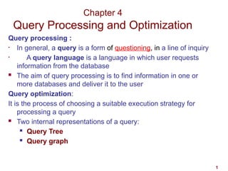
Query processing :
• In general, a query is a form of questioning, in a line of inquiry
• A query language is a language in which user requests
information from the database
 The aim of query processing is to find information in one or
more databases and deliver it to the user
Query optimization:
It is the process of choosing a suitable execution strategy for
processing a query
 Two internal representations of a query:
 Query Tree
 Query graph

Query Processing and Optimization
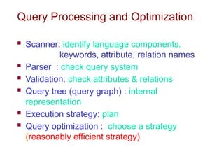
 Scanner: identify language components.
keywords, attribute, relation names
 Parser : check query system
 Validation: check attributes & relations
 Query tree (query graph) : internal
representation
 Execution strategy: plan
 Query optimization : choose a strategy
(reasonably efficient strategy)

Query Processing (cont…)
 Query Processing can be divided into four main phases:
 Decomposition:
 Optimization
 Code generation, and
 Execution
 Decomposition: it is the process of transforming a high
level query into a relational algebra query, and to check
that the query is syntactically and semantically correct.
Query decomposition consists of parsing and validation
4

 Typical stages in query decomposition are:
 Analysis: lexical and syntactical analysis of the query
(correctness).

Query tree will be built for the query containing leaf
node for base relations, one or many non-leaf
nodes for relations produced by relational algebra
operations and root node for the result of the query.
Sequence of operation is from the leaves to the
root.
 Normalization: convert the query into a normalized
form. The predicate WHERE will be converted to
Conjunctive () or Disjunctive () Normal form.
5

 Typical stages in query decomposition(cont…)
 Semantic Analysis: to reject normalized queries that are not
correctly formulated or contradictory.

Incorrect if components do not contribute to generate
result.

Contradictory if the predicate can not be satisfied by any
tuple.
 Simplification: to detect redundant qualifications, eliminate
common sub-expressions, and transform the query to a
semantically equivalent but more easily and effectively
computed form.
 Query Restructuring When more than one translation is
possible, use transformation rules to re arranging nodes so
that the most restrictive condition will be executed first.
6

7
Transformation Rules for Relational Algebra
 Relational algebra operations:

Select, Project , Join, Union, Intersection, Cartesian Poduct
-
refer the text book for detail understanding
 General Transformation rules for relational
algebra
1. Cascade of s: A conjunctive selection condition can be
broken up into a cascade (sequence) of individual s
operations:

s c1 AND c2 AND ... AND cn(R) = sc1 (sc2 (...(scn(R))...) )
2. Commutativity of s:

The s operation is commutative:

sc1 (sc2(R)) = sc2 (sc1(R))
3. Cascade of p: In a cascade (sequence) of p operations, all
but the last one can be ignored:

pList1 (pList2 (...(pListn(R))...) ) = pList1(R)

8
(cont…)
4. Commuting s with p:
 If the selection condition c involves only the
attributes A1, ..., An in the projection list, the two
operations can be commuted:
 pA1, A2, ..., An (sc (R)) = sc (pA1, A2, ..., An (R))
5. Commuting of and X: both are commutative
R c S = S c R, RXS=SXR

9
(cont…)
6. Commuting p with : If projection list is L = {A1, ..., An,
B1, ..., Bm}, where A1, ..., An are attributes of R and
B1, ..., Bm are attributes of S and the join condition c
involves only attributes in L, the two operations can be
commuted as follows:

pL ( R C S ) = (pA1, ..., An (R)) C (p B1, ..., Bm (S))
7. Converting a (s, x) sequence into : If the condition c of
a s that follows a x Corresponds to a join condition,
convert the (s, x) sequence into a as follows:
(sC (R x S)) = (R C S)

Transformation Rules for Relational
Algebra (cont…)
 Reading Assignment
 8. Commutativity of THETA JOIN/Cartesian Product
R X S is equivalent to S X R
Also holds for Equi-Join and Natural-Join
(R c1S)= (S c1R)
 9. Commutativity of SELECTION with THETA JOIN
 If the predicate c1 involves only attributes of one of the
relations (R) being joined, then the Selection and Join
operations commute
10. Commuting SELECTION with SET OPERATIONS
11. Commuting PROJECTION with UNION
10

11
Query Processing
 Query Block:

It is the basic unit that can be translated into the
algebraic operators
 A query block contains a single SELECT-FROM-
WHERE expression, as well as GROUP BY and
HAVING clause if these are part of the block.
 Nested queries within a query are identified as
separate query blocks.

Example: Find the name of employees whose
salary is below the average salary of all employees
who are working at department number 5

12
SELECT FNAME, LNAME
FROM EMPLOYEE
WHERE SALARY < C ( SELECT AVG (SALARY)
FROM EMPLOYEE
WHERE DNO = 5);
SELECT AVG (SALARY)
FROM EMPLOYEE
WHERE DNO = 5
SELECT FNAME, LNAME
FROM EMPLOYEE
WHERE SALARY < C
πFNAME, LNAME (σSALARY<C(EMPLOYEE)) ℱAVGSALARY (σDNO=5 (EMPLOYEE))

13
Basic algorithms for executing query
operations
 External sorting:
 Refers to sorting algorithms that are suitable for large
files of records stored on disk that do not fit entirely in
main memory, such as most database files
 External Sorting Uses Sort-Merge Strategy:
 Starts by sorting small sub files (runs) of the main file
and then merges the sorted runs, creating larger sorted
sub files that are merged in turn
 Sorting Phase:

Number of subfiles (runs) nR = (b/nB)
 Merging phase:

Degree of merging(dM) = Min (nB-1, nR); nP =
(logdM(nR))

14
Sort-Merge strategy (cont…)
 nR: number of initial runs;
 b: number of file blocks;
 nB: available buffer space;
 dM: degree of merging;
 P: number of passes
 The size of a run and number of initial run depends on the
number of file blocks (b) and available buffer space (nB)
 Example: if nB=5 blocks and size of the file=1024 blocks,
 nR=(b/nB)= (1024/5) =205 runs each of size 5 blocks
except the last run which will have 4 blocks.
 Hence, after the sort phase, 205 sorted runs are stored
as temporary subfiles on disk

15
 In the merging phase, the sorted runs are merged during
one or more passes.
 The degree of merging (dM) is the number of runs that
can be merged in each pass.
 dM=min((nB-1) and nR))
 The number of passes=[(logdM
(nR)
)]
 In each pass, one buffer block is needed to hold one block
from each of the runs being merged and one block is
needed for containing one block of the merge result

16
 In the above example, dM=4(four way merging)
 Hence, the 205 initial sorted runs would be merged into:
 52 at the end of the first pass
 13 at the end of the second pass
 4 at the end of the third pass
 1 at the end of the fourth pass
 The minimum dM of 2 gives the worst case performance
of the algorithm, which is

2*b +2(*(b*(log2
(nR)
)
 The first term represents the number of block access for
the sort phase and the second term represents the
number of block access for the merge phase

Use the following logical model to understand the
discussions in this chapter
17

Implementing SELECT operation
18
 There are many options for executing a SELECT
operation
 Some options depend on the file having specific
access paths and may apply only to certain types of
selection conditions
 Examples: Use the logical model provided in the
previous slide to understand the following operations:
(OP1) σSsn=12345689 (EMPLOYEE)
equality comparison on key attribute
(OP2) σDNUMBER > 5 (DEPARMENT)
nonequality comparison on key attribute
(OP3) σDNO=5 (EMPLOYEE)
equality comparison on non key attribute
(OP4) σDNO=5 AND SALARY >30000 AND SEX=F(EMPLOYEE)
conjunctive condition
(OP5) σSsn=123456789 AND PNO=10 (WORKS_ON)
conjunctive condition and composite key

19
Implementing the SELECT Operation (cont…)
 Search Methods for implementing Simple Selection:

S1 Linear search (brute force):

Retrieve every record in the file, and test whether its attribute
values satisfy the selection condition.

S2 Binary search:

If the selection condition involves an equality comparison on a
key attribute on which the file is ordered, binary search (which
is more efficient than linear search) can be used. An example
is OP1 if IDNo is the ordering attribute for EMPLOYEE file

S3 Using a primary index or hash key to retrieve a
single record:

If the selection condition involves an equality comparison on a
key attribute with a primary index (or a hash key), use the
primary index (or the hash key) to retrieve the record.

For Example, OP1 use primary index to retrieve the record

20
Implementing the SELECT Operation (cont…)
 Search Methods for implementing Simple Selection(cont…)
 S4 Using a primary index to retrieve multiple records:

If the comparison condition is >, ≥, <, or ≤ on a key
field with a primary index, use the index to find the
record satisfying the corresponding equality condition,
then retrieve all subsequent records in the (ordered)
file. (see OP2)

S5 Using a clustering index to retrieve multiple
records:

If the selection condition involves an equality
comparison on a non-key attribute with a clustering
index, use the clustering index to retrieve all the
records satisfying the selection condition. (See OP3)

21
Implementing the SELECT Operation
(cont…)

S6: using a secondary index on an equality
comparison:
• This search method can be used to retrieve a single record if
the indexing field is a key (has unique values) or to retrieve
multiple records if the indexing field is not a key
• Search Methods for implementing complex Selection

S7: Conjunctive selection using an individual index :

If an attribute involved in any single simple condition in
the conjunctive condition has an access path that
permits the use of one of the methods S2 to S5, use that
condition to retrieve the records and then check whether
each retrieved record satisfies the remaining simple
conditions in the conjunctive condition

22
Implementing the SELECT Operation (summarized)
 Whenever a single condition specifies the selection, we
can only check whether an access path exists on the
attribute involved in that condition.

If an access path exists, the method corresponding
to that access path is used;

Otherwise, the “brute force” linear search approach
of method S1 is used
 For conjunctive selection conditions, whenever
more than one of the attributes involved in the
conditions have an access path, query optimization
should be done to choose the access path that
retrieves the fewest records in the most efficient way

23
Implementing the SELECT Operation
(summarized)
 Disjunctive selection conditions: This is a situation where
simple conditions are connected by the OR logical
connective rather than AND
 Compared to conjunctive selection, It is much harder to
process and optimize
 Example:s DNO=5 OR SALARY>3000 OR SEX=‘F‘ (EMPLOYEE)
 Little optimization can be done because the records
satisfying the disjunctive condition are the union of the
records satisfying the individual conditions
 Hence, if any of the individual conditions does not have
an access path, we are compelled to use the brute force
approach

24
Implementing the JOIN Operation:
 The join operation is one of the most time
consuming operation in query processing
 Join

two–way join: a join on two files

e.g. R A=B S

multi-way joins: joins involving more than two files

e.g. R A=B S C=D T
 Examples

(OP6): EMPLOYEE DNO=DNUMBER DEPARTMENT

(OP7): DEPARTMENT MGRSSN=SSN EMPLOYEE

25
Implementing the JOIN Operation(cont…)
 Methods for implementing joins:
 J1 Nested-loop join (brute force):

For each record t in R (outer loop), retrieve every
record s from S (inner loop) and test whether the
two records satisfy the join condition t[A] = s[B]
 J2 Single-loop join (Using an access structure to
retrieve the matching records):

If an index (or hash key) exists for one of the two
join attributes — say, B of S — retrieve each record
t in R, one at a time, and then use the access
structure to retrieve directly all matching records s
from S that satisfy s[B] = t[A].

26
Algorithms for SELECT and JOIN
Operations (cont…)
 Implementing the JOIN Operation (cont...):
 Factors affecting JOIN performance
 Available buffer space
 Join selection factor
 Choice of inner VS outer relation
 Selectivity
 Is ratio of the number of records (tuples) that satisfy
the condition to the total number of records (tuples) in
the file (relation

Algorithms for SELECT and JOIN
Operations (cont…)
 is a number between zero and 1
 zero selectivity means no records satisfy the
condition and 1 means all the records satisfy the
condition.
 Although exact selectivities of all conditions may
not be available, estimates of selectivities are
often kept in the DBMS catalog and are used by
the optimizer
27

28
Algorithms for PROJECT and SET
Operations
 Algorithm for PROJECT operations ()
 <attribute list>(R)
1. If <attribute list> has a key of relation R, extract all tuples
from R with only the values for the attributes in <attribute
list>.
2. If <attribute list> does NOT include a key of relation R,
duplicated tuples must be removed from the results.
 Methods to remove duplicate tuples
1. Sorting
2. Hashing

Query Optimization
 Given the database structure, the challenge of query
optimization is to find the sequence of steps that produces
the answer to user request in the most efficient manner
 The performance of a query is affected by the tables or
queries that underlies the query and by the complexity of the
query.
 Given a request for data manipulation or retrieval, an
optimizer will choose an optimal plan for evaluating the
request from among the available alternative strategies.
 There are many ways (access paths) for accessing desired
file/record. The optimizer tries to select the most efficient
(cheapest) access path for accessing the data.
 DBMS is responsible to pick the best execution strategy
based on various considerations.
29

Approaches to Query Optimization
 Heuristics Approach
 The heuristic approach uses the knowledge of the
characteristics of the relational algebra operations and
the relationship between the operators to optimize the
query.
 Thus the heuristic approach of optimization will make
use of:

Properties of individual operators

Association between operators

Query Tree: a graphical representation of the
operators, relations, attributes and predicates and
processing sequence during query processing.
30

31
Using Heuristics in Query Optimization
 Process for heuristics optimization
1. The parser of a high-level query generates an initial
internal representation;
2. Apply heuristics rules to optimize the internal
representation.
3. A query execution plan is generated to execute groups of
operations based on the access paths available on the files
involved in the query
 The main heuristic is to apply first the operations that
reduce the size of intermediate results
 E.g., Apply SELECT and PROJECT operations before
applying the JOIN or other binary operations

32
Using Heuristics in Query Optimization
(cont…)
 Heuristic Optimization of Query Trees:
 The same query could correspond to many different
relational algebra expressions — and hence many different
query trees.
 The task of heuristic optimization of query trees is to find a
final query tree that is efficient to execute.
 Example: Find the name of all employees who are working
in AQUARIUS project and born before ‘1957-12-31’
Q: SELECT LNAME
FROM EMPLOYEE, WORKS_ON,
PROJECT
WHERE PNAME = ‘AQUARIUS’ AND
PNMUBER=PNO AND ESSN=SSN
AND BDATE < ‘1957-12-31’;

Steps in Typical Heuristic optimization
1. Deconstruct conjunctive selections into a sequence of
single selection operations (Equiv. rule 1.).
2. Move selection operations down the query tree for the
earliest possible execution
3. Execute first those selection and join operations that will
produce the smallest relations
4. Replace Cartesian product operations that are followed by
a selection condition by join operations
5. Deconstruct and move as far down the tree as possible
lists of projection attributes, creating new projections
where needed
33

34
Steps in converting a query tree during heuristic optimization:
Initial query tree for the query Q on slide 32

35
Moving the select operation down the tree

36
Applying the more restrictive select operation first

37
Replacing Cartesian product and select with join

38
Moving project operations down the query tree

39
Heuristics in Query Optimization (cont…)
 Summary of Heuristics for Algebraic Optimization:
1. The main heuristic is to apply first the operations that
reduce the size of intermediate results
2. Perform select operations as early as possible to reduce
the number of tuples and perform project operations as
early as possible to reduce the number of attributes. (This
is done by moving select and project operations as far
down the tree as possible.)
3. The select and join operations that are most restrictive
should be executed before other similar operations. (This
is done by reordering the leaf nodes of the tree among
themselves and adjusting the rest of the tree
appropriately.)

40
Using Selectivity and Cost Estimates in
Query Optimization
 Cost-based query optimization:
 Estimate and compare the costs of executing a query
using different execution strategies and choose the
strategy with the lowest cost estimate
 Cost Components for Query Execution
1. Access cost to secondary storage
2. Computation cost
3. Memory usage cost
4. Communication cost
 Note: Different database systems may focus on different
cost components.


41
Using Selectivity and Cost Estimates in
Query Optimization (cont…)
 Catalog Information Used in Cost Functions
 Information about the size of a file

number of records (tuples) (r),

record size (R),

number of blocks (b)

blocking factor (bfr)
 Information about indexes and indexing attributes of a file

Number of levels (x) of each multilevel index

Number of first-level index blocks (bI1)

Number of distinct values (d) of an attribute

Selectivity (sl) of an attribute

42
Semantic Query Optimization
 Semantic Query Optimization:
 Uses constraints specified on the database schema in order to
modify one query into another query that is more efficient to
execute
 Read more about:
 Sematic query optimization and
 Semantic Query Optimization (SQO) Techniques

Chapter 4 - Query Processing and Optimization.pptx

More Related Content

Similar to Chapter 4 - Query Processing and Optimization.pptx

More from ahmed518927

Recently uploaded

Chapter 4 - Query Processing and Optimization.pptx