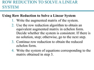
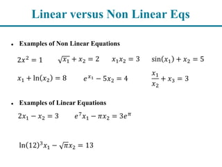
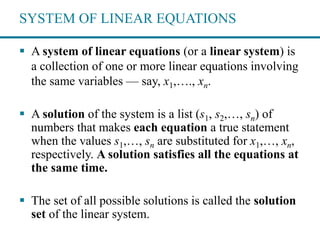
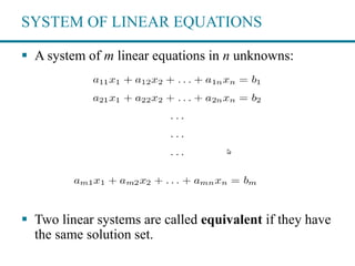
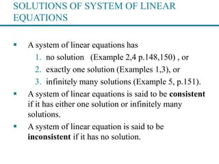
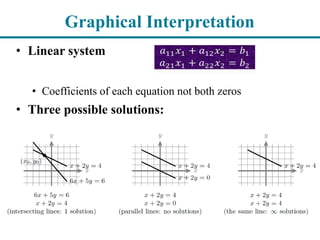
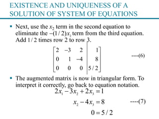
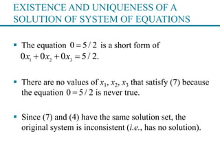
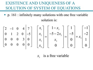
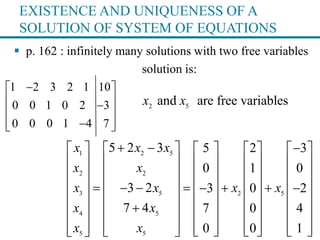
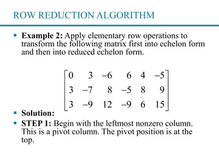
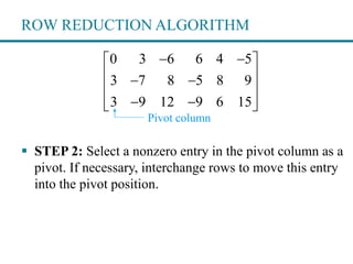
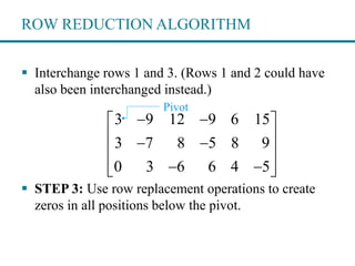
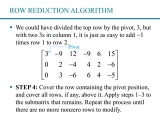
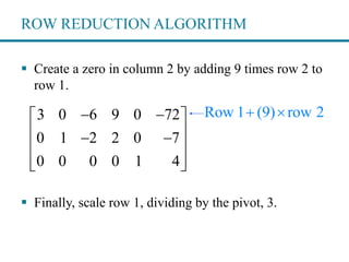
The document provides information about linear systems and matrices. It begins by defining linear and non-linear equations. It then discusses systems of linear equations, their graphical and geometric interpretations, and the three possible solutions: no solution, a unique solution, or infinitely many solutions. The document also covers matrix notation for representing linear systems, elementary row operations for transforming systems, and determining whether a system has a solution and whether that solution is unique.

1. LINEAR SYSTEMS
AND
MATRICES

2. The material in these lecture notes
comes mainly from the instructor’s
Power Point Slides that accompany the
book “Linear Equations in Linear
Algebra” by David C. Lay

3. Linear versus Non Linear Eqs
 Examples of Non Linear Equations
 Examples of Linear Equations

4. Why linear?
 Linear because:
 the unknowns only appear to the first power
 there aren’t any unknowns in the denominator of a
fraction.
 the unknowns only occur in numerators
 there are no products and/or ratios of unknowns.

5. SYSTEMS OF LINEAR EQUATIONS
 SYSTEMS OF
LINEAR EQUATIONS

6. LINEAR EQUATION
 A linear equation in the variables is an
equation that can be written in the form
,
where b and the coefficients are real or
complex numbers that are usually known in advance.
 A solution of a linear equation is a list (s1, s2,…, sn) of
numbers that makes the equation a true statement when
the values s1,…, sn are substituted for x1,…, xn,
respectively.
1
, , n
x x
1 1 2 2 n n
a x a x a x b   
1
, , n
a a
1 2
, , , : unknownsn
x x x

7. SYSTEM OF LINEAR EQUATIONS
 A system of linear equations (or a linear system) is
a collection of one or more linear equations involving
the same variables — say, x1,…., xn.
 A solution of the system is a list (s1, s2,…, sn) of
numbers that makes each equation a true statement
when the values s1,…, sn are substituted for x1,…, xn,
respectively. A solution satisfies all the equations at
the same time.
 The set of all possible solutions is called the solution
set of the linear system.

8. SYSTEM OF LINEAR EQUATIONS
 A system of m linear equations in n unknowns:
 Two linear systems are called equivalent if they have
the same solution set.

9. SOLUTIONS OF SYSTEM OF LINEAR
EQUATIONS
 A system of linear equations has
1. no solution (Example 2,4 p.148,150) , or
2. exactly one solution (Examples 1,3), or
3. infinitely many solutions (Example 5, p.151).
 A system of linear equations is said to be consistent
if it has either one solution or infinitely many
solutions.
 A system of linear equation is said to be
inconsistent if it has no solution.

10. Graphical Interpretation
• Linear system
• Coefficients of each equation not both zeros
• Three possible solutions:

11. Geometrical Interpretation
• Planes
• Possible solutions include:
• The two planes might be coincident or they can intersect
in a line;
• Infinite number of solutions
• The two planes can be parallel
• No solution
• How about the same case for (3 x 3) system?
Examples 6, 7 p.152 to 154

12. Geometric Interpretation
A unique solution
(a single point where the 3
plans intersect)
No solution
(no intersection at all;
Planes are parallel)
Infinitely many solutions
(intersection of planes forms
a line;
there is infinitely many point
on a line)
See (p.156) – Problem 33 for more examples

13. Classification of Linear Systems
• Consistent – system has at least one solution
• Inconsistent – system has no solution
• A consistent system has either one solution or an infinite number
of solutions (i.e. it is not possible for a linear system to have, for
example, exactly five solutions)
• Just-determined system: same equations and unknowns
• Over-determined system: more equations than unknowns
• Under-determined system: fewer equations than unknowns

14. Problems 3.1
p. 155
Problems : 1 to 22
p.156 – Observe Problem 33 :
Cases where there is
no solutions
exactly one solution
infinitely many solutions

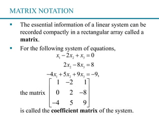
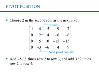
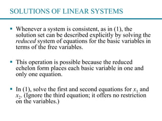
15. Equivalent Linear Systems
Two linear systems are EQUIVALENT
if and only if
they have the same solution sets.
Ex: x – y = 1 and x – y = 1
x + y = 3 y = 1
vector [2, 1] is the unique solution for both systems
Note that the second system is easier to solve !

16. MATRIX NOTATION
 The essential information of a linear system can be
recorded compactly in a rectangular array called a
matrix.
 For the following system of equations,
the matrix
is called the coefficient matrix of the system.
1 2 1
0 2 8
4 5 9
 
 
 
  
1 2 3
2 3
1 2 3
2 0
2 8 8
4 5 9 9,
x x x
x x
x x x
  
 
    

17. MATRIX NOTATION
 An augmented matrix of a system consists of the
coefficient matrix with an added column containing
the constants from the right sides of the equations.
 For the given system of equations,
is called the augmented matrix.
1 2 1 0
0 2 8 8
4 5 9 9
 
 
 
   

18. MATRIX SIZE
 The size of a matrix tells how many rows and
columns it has. If m and n are positive numbers, an
m n matrix is a rectangular array of numbers with
m rows and n columns. (The number of rows
always comes first.)
 The basic strategy for solving a linear system is
to replace one system with an equivalent system
(i.e., one with the same solution set) that is easier
to solve.


19. SOLVING SYSTEM OF EQUATIONS
 Example 1: Solve the given system of equations.
----(1)
----(2)
----(3)
 Solution: The elimination procedure is shown here
with and without matrix notation, and the results are
placed side by side for comparison.
1 2 3
2 3
1 2 3
2 0
2 8 8
4 5 9 9
x x x
x x
x x x
  
 
    

20. SOLVING SYSTEM OF EQUATIONS
 Keep x1 in the first equation and eliminate it from the
other equations. To do so, add 4 times equation 1 to
equation 3.
1 2 3
2 3
1 2 3
2 0
2 8 8
4 5 9 9
x x x
x x
x x x
  
 
    
1 2 1 0
0 2 8 8
4 5 9 9
 
 
 
   
1 2 3
1 2 3
2 3
4 8 4 0
4 5 9 9
3 13 9
x x x
x x x
x x
  
    
   

21. SOLVING SYSTEM OF EQUATIONS
 The result of this calculation is written in place of the
original third equation.
 Now, multiply equation 2 by in order to obtain 1
as the coefficient for x2.
1 2 3
2 3
2 3
2 0
2 8 8
3 13 9
x x x
x x
x x
  
 
   
1 2 1 0
0 2 8 8
0 3 13 9
 
 
 
   
1/ 2

22. SOLVING SYSTEM OF EQUATIONS
 Use the x2 in equation 2 to eliminate the in
equation 3.
1 2 3
2 3
2 3
2 0
4 4
3 13 9
x x x
x x
x x
  
 
   
1 2 1 0
0 1 4 4
0 3 13 9
 
 
 
   
2
3x
2 3
2 3
3
3 12 12
3 13 9
3
x x
x x
x
 
   


23. SOLVING SYSTEM OF EQUATIONS
 The new system has a triangular form.
 Now, you want to eliminate the term from
equation 1, but it is more efficient to use the x3 term in
equation 3 first to eliminate the and x3 terms in
equations 2 and 1.
1 2 3
2 3
3
2 0
4 4
3
x x x
x x
x
  
 

1 2 1 0
0 1 4 4
0 0 1 3
 
 
 
  
2
2x
3
4x

24. SOLVING SYSTEM OF EQUATIONS
3
2 3
2
4 12
4 4
16
x
x x
x

 

 Now, combine the results of these two operations.
3
1 2 3
1 2
3
2 0
2 3
x
x x x
x x
  
  
  
1 2
2
3
2 3
16
3
x x
x
x
  


1 2 0 3
0 1 0 16
0 0 1 3
  
 
 
  

25. SOLVING SYSTEM OF EQUATIONS
 Move back to the x2 in equation 2, and use it to
eliminate the above it. Because of the previous
work with x3, there is now no arithmetic involving x3
terms. Add 2 times equation 2 to equation 1 and obtain
the system:
1
2
3
29
16
3
x
x
x



1 0 0 29
0 1 0 16
0 0 1 3
 
 
 
  
2
2x

26. SOLVING SYSTEM OF EQUATIONS
 Thus, the only solution of the original system is
(29,16,3). To verify that (29,16,3) is a solution,
substitute these values into the left side of the original
system, and compute.
 The results agree with the right side of the original
system, so (29,16,3) is a solution of the system.
(29) 2(16) (3) 29 32 3 0
2(16) 8(3) 32 24 8
4(29) 5(16) 9(3) 116 80 27 9
     
   
        

27. ELEMENTARY ROW OPERATIONS
 Elementary row operations include the following:
1. (Replacement) Replace one row by the sum of
itself and a multiple of another row.
2. (Interchange) Interchange two rows.
3. (Scaling) Multiply all entries in a row by a
nonzero constant.
 Two matrices are called row equivalent if there is a
sequence of elementary row operations that
transforms one matrix into the other.

28. ELEMENTARY ROW OPERATIONS
 It is important to note that row operations are
reversible.
 If the augmented matrices of two linear systems are
row equivalent, then the two systems have the same
solution set.
 Elementary row operations guarantee that all
intermediate systems (matrices) obtained through
this process have the same set of solutions.
 Elementary row operations allow transformation of
an original system into an equivalent system which
is easier to solve.

29. ELEMENTARY ROW OPERATIONS
 Two fundamental questions about a linear system
are as follows:
1. Is the system consistent; that is, does at least
one solution exist?
2. If a solution exists, is it the only one; that is, is
the solution unique?

30. EXISTENCE AND UNIQUENESS OF A
SOLUTION OF SYSTEM OF EQUATIONS
 Example 2: Determine if the following system is
consistent.
----(4)
 Solution: The augmented matrix is
2 3
1 2 3
1 2 3
4 8
2 3 2 1
5 8 7 1
x x
x x x
x x x
 
  
  
0 1 4 8
2 3 2 1
5 8 7 1
 
 
 
  

31. EXISTENCE AND UNIQUENESS OF A
SOLUTION OF SYSTEM OF EQUATIONS
 To obtain an x1 in in the first equation, interchange rows
1 and 2.
 To eliminate the 5x1 term in the third equation, add
times row 1 to row 3.
----(5)
2 3 2 1
0 1 4 8
5 8 7 1
 
 
 
  
5/ 2
2 3 2 1
0 1 4 8
0 1/ 2 2 3/ 2
 
 
 
   

32. EXISTENCE AND UNIQUENESS OF A
SOLUTION OF SYSTEM OF EQUATIONS
 Next, use the x2 term in the second equation to
eliminate the term from the third equation.
Add times row 2 to row 3.
----(6)
 The augmented matrix is now in triangular form. To
interpret it correctly, go back to equation notation.
----(7)
2
(1/ 2)x
1/ 2
2 3 2 1
0 1 4 8
0 0 0 5 / 2
 
 
 
  
1 2 3
2 3
2 3 2 1
4 8
0 5 / 2
x x x
x x
  
 


33. EXISTENCE AND UNIQUENESS OF A
SOLUTION OF SYSTEM OF EQUATIONS
 The equation is a short form of
 There are no values of x1, x2, x3 that satisfy (7) because
the equation is never true.
 Since (7) and (4) have the same solution set, the
original system is inconsistent (i.e., has no solution).
0 5/ 2
1 2 3
0 0 0 5/ 2.x x x  
0 5/ 2

34. EXISTENCE AND UNIQUENESS OF A
SOLUTION OF SYSTEM OF EQUATIONS
 p. 161 : infinitely many solutions with one free variable
solution is:
1 3
2 3
3
3 3
4
1 1 1
5 2 5 2
0 1
0 0 0
x x
x x
x
x x
x
        
          
         
       
       
      
2 1 0 4 7
0 1 2 0 5
0 0 0 3 0
0 0 0 0 0
 
 
 
 
 
 
3
is a free variablex

35. EXISTENCE AND UNIQUENESS OF A
SOLUTION OF SYSTEM OF EQUATIONS
 p. 162 : infinitely many solutions with two free variables
solution is:
1 2 5
2 2
3 5 2 5
4 5
5 5
5 2 3 5 2 3
0 1 0
3 2 3 0 2
7 4 7 0 4
0 0 1
x x x
x x
x x x x
x x
x x
           
         
         
               
                  
                 
1 2 3 2 1 10
0 0 1 0 2 3
0 0 0 1 4 7
 
 
 
  
2 5
and are free variablesx x

36. Problems 3.2
p. 165
Problems : 1 to 27

37. SOLVING LINEAR SYSTEMS
 DIRECT METHODS FOR
SOLVING LINEAR
SYSTEMS

38. SOLVING LINEAR SYSTEMS
Row Reduction,
Echelon Form, and
Reduced Echelon Form

39. ECHELON FORM
 A rectangular matrix is in echelon form (or row
echelon form) if it has the following three
properties:
1. All nonzero rows are above any rows of all
zeros.
2. Each leading entry of a row is in a column to
the right of the leading entry of the row above
it.
3. All entries in a column below a leading entry
are zeros.

40. REDUCED ECHELON FORM
 If a matrix in echelon form satisfies the following
additional conditions, then it is in reduced echelon
form (or reduced row echelon form):
4. The leading entry in each nonzero row is 1.
5. Each leading 1 is the only nonzero entry in its
column.
 An echelon matrix (respectively, reduced echelon
matrix) is one that is in echelon form (respectively,
reduced echelon form.)

41. Examples: Echelon Form
7 1 4 3 0 2 0
0 0 3 8 4 3 2
0 0 0 2 2 1 2
0 0 0 0 0 1 3
0 0 0 0 0 0 0
 
  
 
 
 
  
0 3 1 4 3
0 0 1 6 5
0 0 0 0 1
 
 
 
  
2 3 1 4 0
0 5 1 0 5
0 0 3 0 1
 
 
 
  
1 2 3
0 6 1
 
 
 
1 0 3
0 1 1
 
  
9 0 0 2
0 0 3 6
0 0 0 7
0 0 0 0
 
 
 
 
 
 
2 1 0 1
0 3 9 4
0 0 2 0
0 0 0 4
 
 
 
 
 
 
1 4 3
0 0 2
 
 
 

42. Examples: Reduced Echelon Form
1 2 0 1 1
0 0 1 3 4
0 0 0 0 0
 
 
 
  
1 0 0 2
0 1 0 1
0 0 1 3
 
 
 
  
0 1 0 4 0
0 0 1 6 0
0 0 0 0 1
 
 
 
  
1 0 0 4 0
0 1 0 0 5
0 0 1 0 1
 
 
 
  
1 0 0 1
0 1 0 4
0 0 1 0
0 0 0 0
 
 
 
 
 
 
1 4 0
0 0 1
 
 
 
1 0 3
0 1 1
 
 
 
1 0 0 0
0 1 0 0
0 0 1 0
0 0 0 1
 
 
 
 
 
 1 0 0 4 3
0 1 0 2 5
0 0 1 1 1
 
 
 
  
1 0
0 1
 
 
 

43. Examples: Not Echelon Form
0 1 0 4 0
3 0 1 6 0
0 0 0 0 1
 
 
 
  
0 0 0 1 1
0 0 1 3 4
0 0 0 0 0
 
 
 
  
1 0 0 2
0 0 0 0
0 0 1 3
 
 
 
  
1 0 0 0
0 1 0 0
0 0 1 0
1 0 0 1
 
 
 
 
 
 
3 0 0 4 0
0 1 0 0 5
0 2 1 0 1
 
 
 
  
7 0 0 1
0 1 0 4
0 0 3 0
0 0 2 0
 
 
 
 
 
 
1 4 0
2 0 1
 
 
 
0 0
0 1
 
 
 
4 3 3
2 1 1
  
   
2 5 0 4 3
0 1 0 2 5
0 3 1 1 1
 
 
 
  

44. REDUCED ECHELON FORM
 Any nonzero matrix may be row reduced (i.e.,
transformed by elementary row operations) into more
than one matrix in echelon form, using different
sequences of row operations. However, the reduced
echelon form one obtains from a matrix is unique.
Theorem 1: Uniqueness of the Reduced Echelon
Form
Each matrix is row equivalent to one and only one
reduced echelon matrix.

45. PIVOT POSITION
 If a matrix A is row equivalent to an echelon matrix
U, we call U an echelon form (or row echelon form)
of A; if U is in reduced echelon form, we call U the
reduced echelon form of A.
 A pivot position in a matrix A is a location in A that
corresponds to a leading 1 in the reduced echelon
form of A. A pivot column is a column of A that
contains a pivot position.

46. PIVOT POSITION
 Example 1: Row reduce the matrix A below to
echelon form, and locate the pivot columns of A.
 Solution: The top of the leftmost nonzero column is
the first pivot position. A nonzero entry, or pivot,
must be placed in this position.
0 3 6 4 9
1 2 1 3 1
2 3 0 3 1
1 4 5 9 7
A
  
   
 
   
   

47. PIVOT POSITION
 Now, interchange rows 1 and 4.
 Create zeros below the pivot, 1, by adding multiples
of the first row to the rows below, and obtain the next
matrix.
1 4 5 9 7
1 2 1 3 1
2 3 0 3 1
0 3 6 4 9
  
   
 
   
   
Pivot
Pivot column

48. PIVOT POSITION
 Choose 2 in the second row as the next pivot.
 Add times row 2 to row 3, and add times
row 2 to row 4.
1 4 5 9 7
0 2 4 6 6
0 5 10 15 15
0 3 6 4 9
  
  
 
  
   
Pivot
Next pivot column
5/ 2 3/ 2

49. PIVOT POSITION
 There is no way a leading entry can be created in
column 3. But, if we interchange rows 3 and 4, we
can produce a leading entry in column 4.
1 4 5 9 7
0 2 4 6 6
0 0 0 0 0
0 0 0 5 0
  
  
 
 
  

50. PIVOT POSITION
1 4 5 9 7
0 2 4 6 6
0 0 0 5 0
0 0 0 0 0
  
  
 
 
 
 
 The matrix is in echelon form and thus reveals that
columns 1, 2, and 4 of A are pivot columns.
Pivot
Pivot columns

51. PIVOT POSITION
0 3 6 4 9
1 2 1 3 1
2 3 0 3 1
1 4 5 9 7
A
  
   
 
   
   
 The pivots in the example are 1, 2 and .
Pivot positions
Pivot columns
5

52. ROW REDUCTION ALGORITHM
 Example 2: Apply elementary row operations to
transform the following matrix first into echelon form
and then into reduced echelon form.
 Solution:
 STEP 1: Begin with the leftmost nonzero column.
This is a pivot column. The pivot position is at the
top.
0 3 6 6 4 5
3 7 8 5 8 9
3 9 12 9 6 15
  
  
 
   

53. ROW REDUCTION ALGORITHM
 STEP 2: Select a nonzero entry in the pivot column as a
pivot. If necessary, interchange rows to move this entry
into the pivot position.
0 3 6 6 4 5
3 7 8 5 8 9
3 9 12 9 6 15
  
  
 
   
Pivot column

54. ROW REDUCTION ALGORITHM
 Interchange rows 1 and 3. (Rows 1 and 2 could have
also been interchanged instead.)
 STEP 3: Use row replacement operations to create
zeros in all positions below the pivot.
3 9 12 9 6 15
3 7 8 5 8 9
0 3 6 6 4 5
  
  
 
   
Pivot

55. ROW REDUCTION ALGORITHM
 We could have divided the top row by the pivot, 3, but
with two 3s in column 1, it is just as easy to add
times row 1 to row 2.
 STEP 4: Cover the row containing the pivot position,
and cover all rows, if any, above it. Apply steps 1–3 to
the submatrix that remains. Repeat the process until
there are no more nonzero rows to modify.
1
3 9 12 9 6 15
0 2 4 4 2 6
0 3 6 6 4 5
  
  
 
   
Pivot

56. ROW REDUCTION ALGORITHM
 With row 1 covered, step 1 shows that column 2 is the
next pivot column; for step 2, select as a pivot the “top”
entry in that column.
 For step 3, we could insert an optional step of dividing
the “top” row of the submatrix by the pivot, 2. Instead,
we add times the “top” row to the row below.
3 9 12 9 6 15
0 2 4 4 2 6
0 3 6 6 4 5
  
  
 
   
Pivot
New pivot column
3/ 2

57. ROW REDUCTION ALGORITHM
 This produces the following matrix.
 When we cover the row containing the second pivot
position for step 4, we are left with a new submatrix that
has only one row.
3 9 12 9 6 15
0 2 4 4 2 6
0 0 0 0 1 4
  
  
 
  
3 9 12 9 6 15
0 2 4 4 2 6
0 0 0 0 1 4
  
  
 
  

58. ROW REDUCTION ALGORITHM
 Steps 1–3 require no work for this submatrix, and we
have reached an echelon form of the full matrix. We
perform one more step to obtain the reduced echelon
form.
 STEP 5: Beginning with the rightmost pivot and
working upward and to the left, create zeros above
each pivot. If a pivot is not 1, make it 1 by a scaling
operation.
 The rightmost pivot is in row 3. Create zeros above it,
adding suitable multiples of row 3 to rows 2 and 1.

59. ROW REDUCTION ALGORITHM
3 9 12 9 0 9
0 2 4 4 0 14
0 0 0 0 1 4
   
  
 
  
 The next pivot is in row 2. Scale this row, dividing by
the pivot.
Row 1 ( 6) row 3  
Row 2 ( 2) row 3  
3 9 12 9 0 9
0 1 2 2 0 7
0 0 0 0 1 4
   
  
 
  
1
Row scaled by
2

60. ROW REDUCTION ALGORITHM
 Create a zero in column 2 by adding 9 times row 2 to
row 1.
 Finally, scale row 1, dividing by the pivot, 3.
Row 1 (9) row 2 3 0 6 9 0 72
0 1 2 2 0 7
0 0 0 0 1 4
  
  
 
  

61. ROW REDUCTION ALGORITHM
 This is the reduced echelon form of the original
matrix.
 The combination of steps 1–4 is called the forward
phase of the row reduction algorithm. Step 5, which
produces the unique reduced echelon form, is called
the backward phase.
1 0 2 3 0 24
0 1 2 2 0 7
0 0 0 0 1 4
  
  
 
  
1
Row scaled by
3

62. SOLUTIONS OF LINEAR SYSTEMS
 The row reduction algorithm leads to an explicit
description of the solution set of a linear system when
the algorithm is applied to the augmented matrix of
the system.
 Suppose that the augmented matrix of a linear system
has been transformed into the equivalent reduced
echelon form.
1 0 5 1
0 1 1 4
0 0 0 0
 
 
 
  

63. SOLUTIONS OF LINEAR SYSTEMS
 There are 3 variables because the augmented matrix
has four columns. The associated system of equations
is
----(1)
 The variables x1 and x2 corresponding to pivot
columns in the matrix are called basic variables. The
other variable, x3, is called a free variable.
1 3
2 3
5 1
4
0 0
x x
x x
 
 


64. SOLUTIONS OF LINEAR SYSTEMS
 Whenever a system is consistent, as in (1), the
solution set can be described explicitly by solving the
reduced system of equations for the basic variables in
terms of the free variables.
 This operation is possible because the reduced
echelon form places each basic variable in one and
only one equation.
 In (1), solve the first and second equations for x1 and
x2. (Ignore the third equation; it offers no restriction
on the variables.)

65. SOLUTIONS OF LINEAR SYSTEMS
----(2)
 The statement “x3 is free” means that you are free to
choose any value for x3. Once that is done, the formulas
in (2) determine the values for x1 and x2. For instance,
when , the solution is (1,4,0); when , the
solution is (6,3,1).
 Each different choice of x3 determines a (different)
solution of the system, and every solution of the system
is determined by a choice of x3.
3
0x  3
1x 
1 3
2 3
3
1 5
4
is free
x x
x x
x
 
 

66. PARAMETRIC DESCRIPTIONS OF
SOLUTION SETS
 The description in (2) is a parametric description of
solutions sets in which the free variables act as
parameters.
 Solving a system amounts to finding a parametric
description of the solution set or determining that the
solution set is empty.
 Whenever a system is consistent and has free
variables, the solution set has many parametric
descriptions.

67. PARAMETRIC DESCRIPTIONS OF
SOLUTION SETS
 For instance, in system (1), add 5 times equation 2 to
equation 1 and obtain the following equivalent
system.
 We could treat x2 as a parameter and solve for x1 and
x3 in terms of x2, and we would have an accurate
description of the solution set.
 When a system is inconsistent, the solution set is
empty, even when the system has free variables. In
this case, the solution set has no parametric
representation.
1 2
2 3
5 21
4
x x
x x
 
 

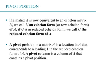
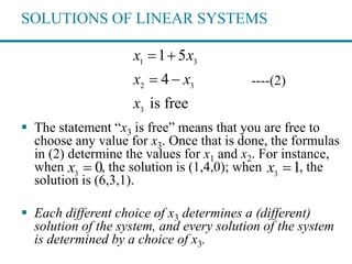
68. EXISTENCE AND UNIQUENESS THEOREM
Theorem 2: Existence and Uniqueness Theorem
A linear system is consistent if and only if the
rightmost column of the augmented matrix is not a
pivot column—i.e., if and only if an echelon form of
the augmented matrix has no row of the form
[0 … 0 b] with b nonzero.
 If a linear system is consistent, then the solution set
contains either (i) a unique solution, when there are
no free variables, or (ii) infinitely many solutions,
when there is at least one free variable.

69. ROW REDUCTION TO SOLVE A LINEAR
SYSTEM
Using Row Reduction to Solve a Linear System
1. Write the augmented matrix of the system.
2. Use the row reduction algorithm to obtain an
equivalent augmented matrix in echelon form.
Decide whether the system is consistent. If there is
no solution, stop; otherwise, go to the next step.
3. Continue row reduction to obtain the reduced
echelon form.
4. Write the system of equations corresponding to the
matrix obtained in step 3.

70. ROW REDUCTION TO SOLVE A LINEAR
SYSTEM
5. Rewrite each nonzero equation from step 4 so
that its one basic variable is expressed in terms of
any free variables appearing in the equation.

71. Problems 3.3
p. 174
Problems : 1 to 30