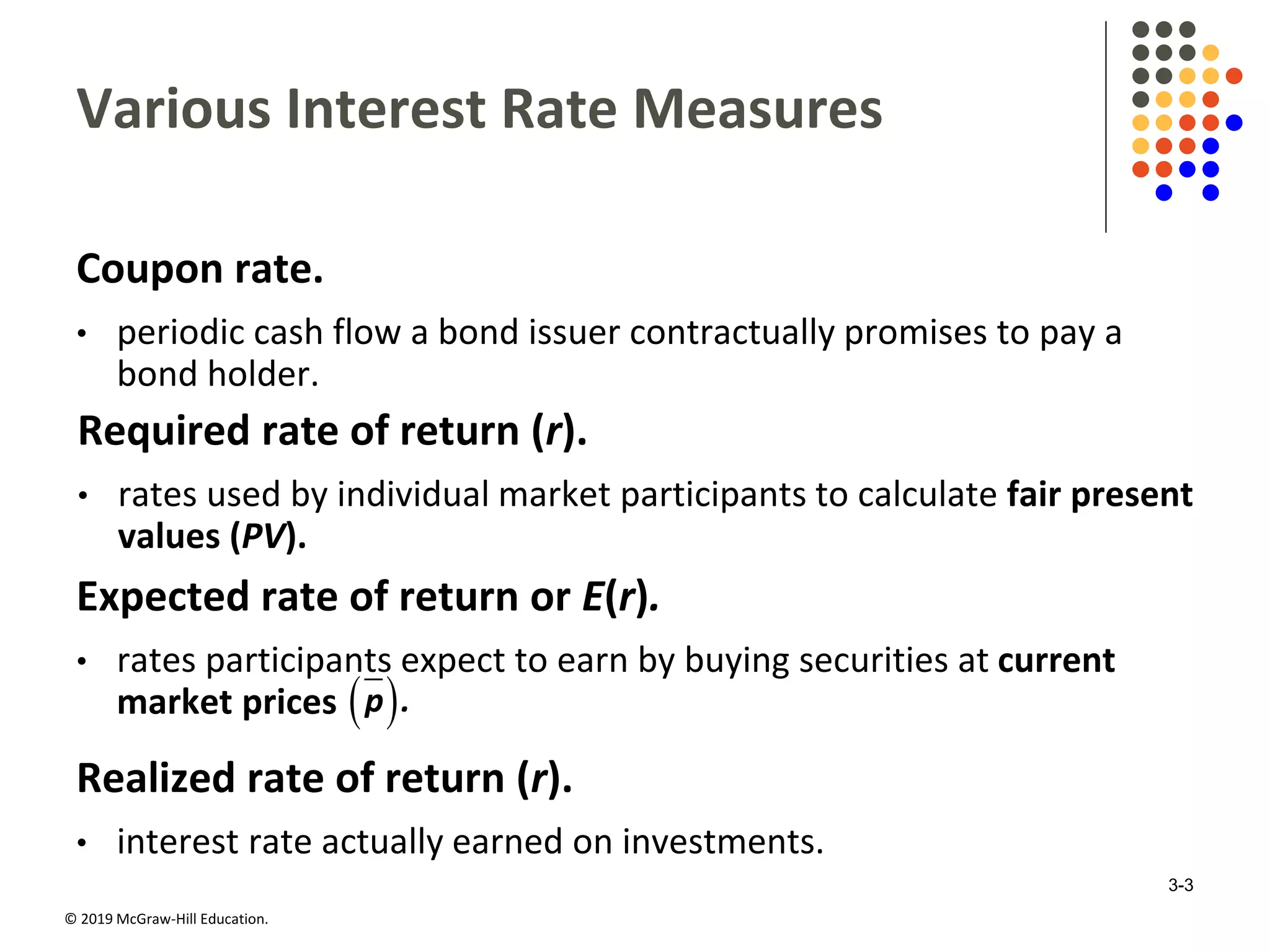
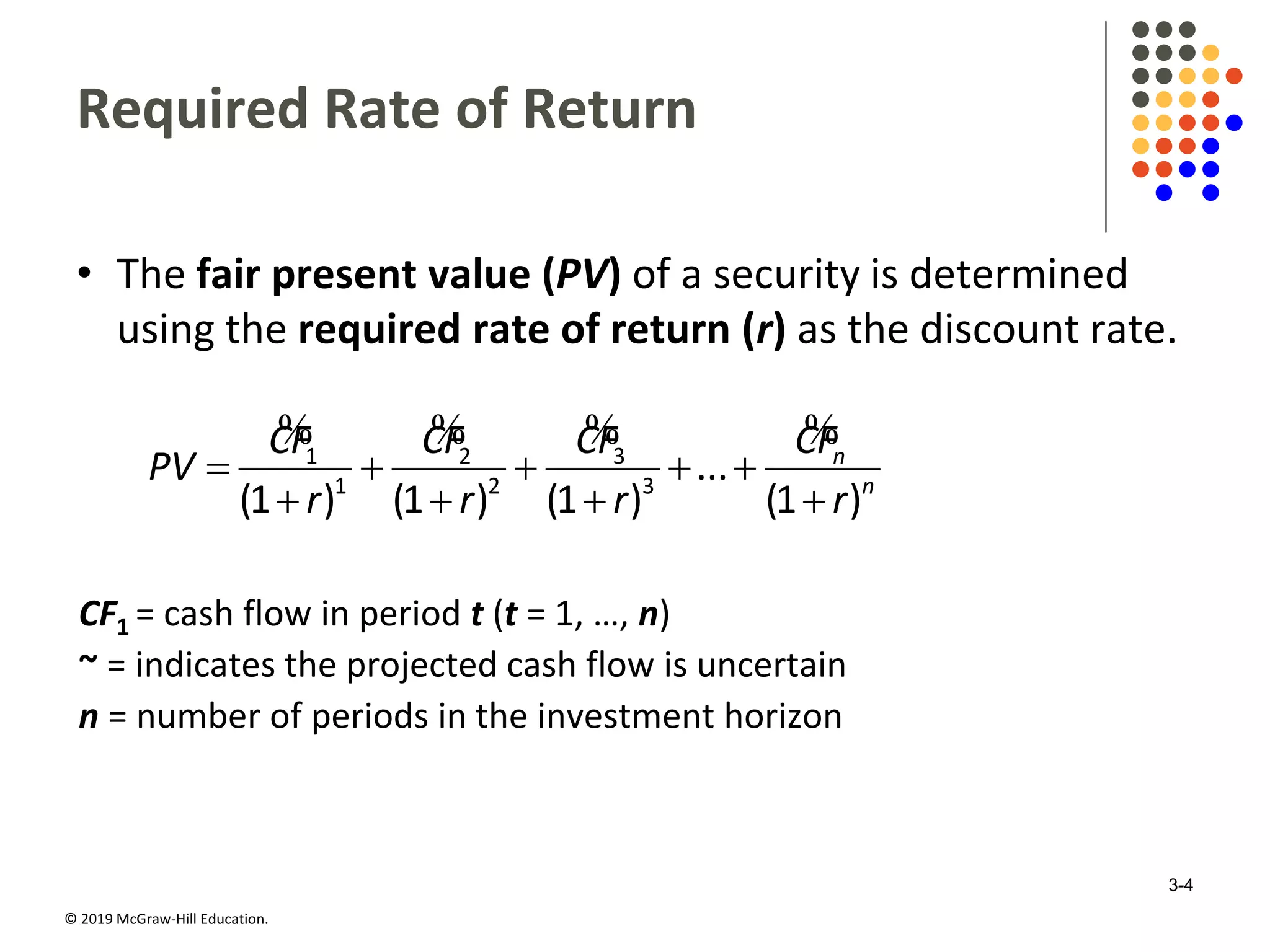
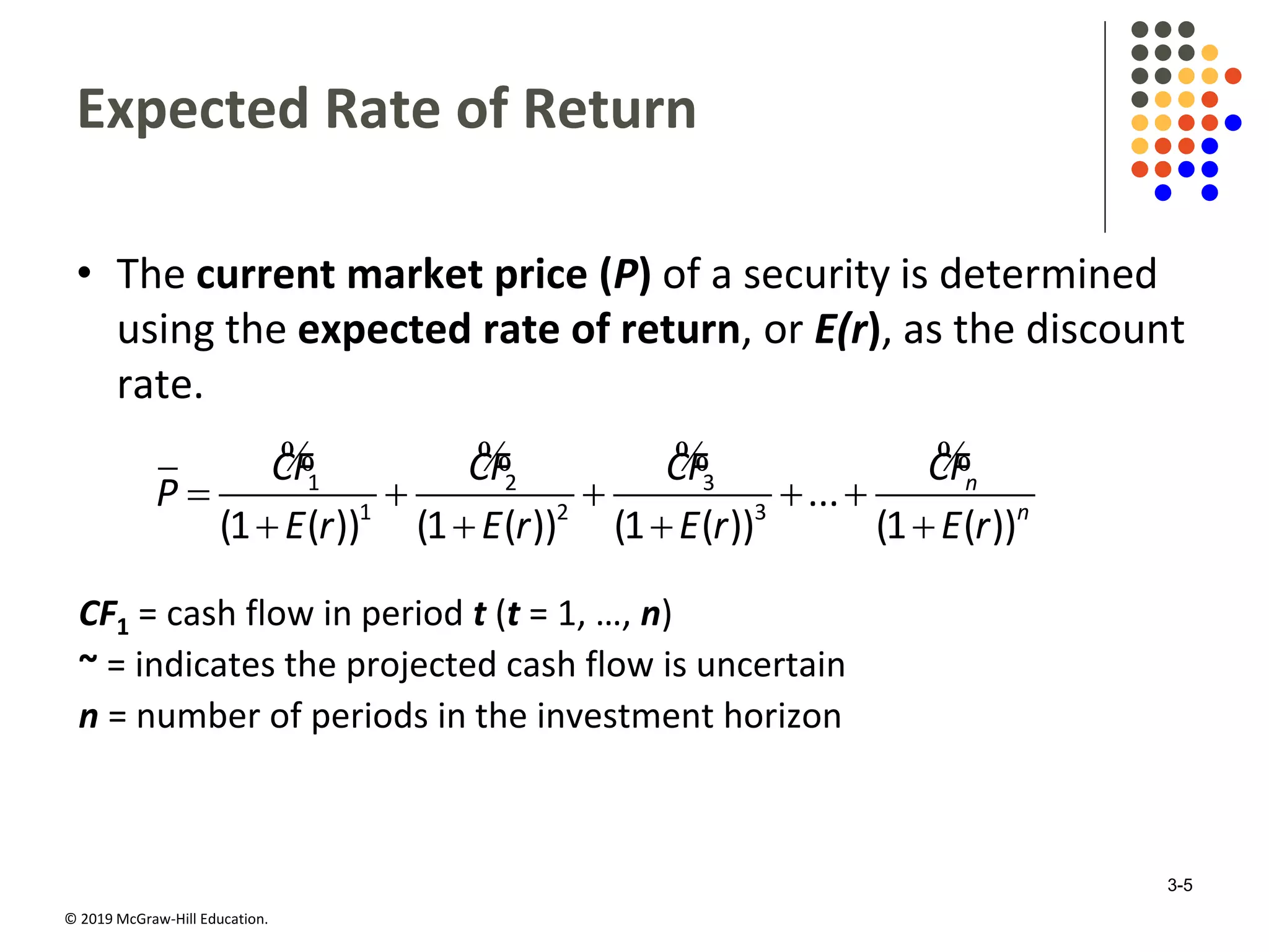
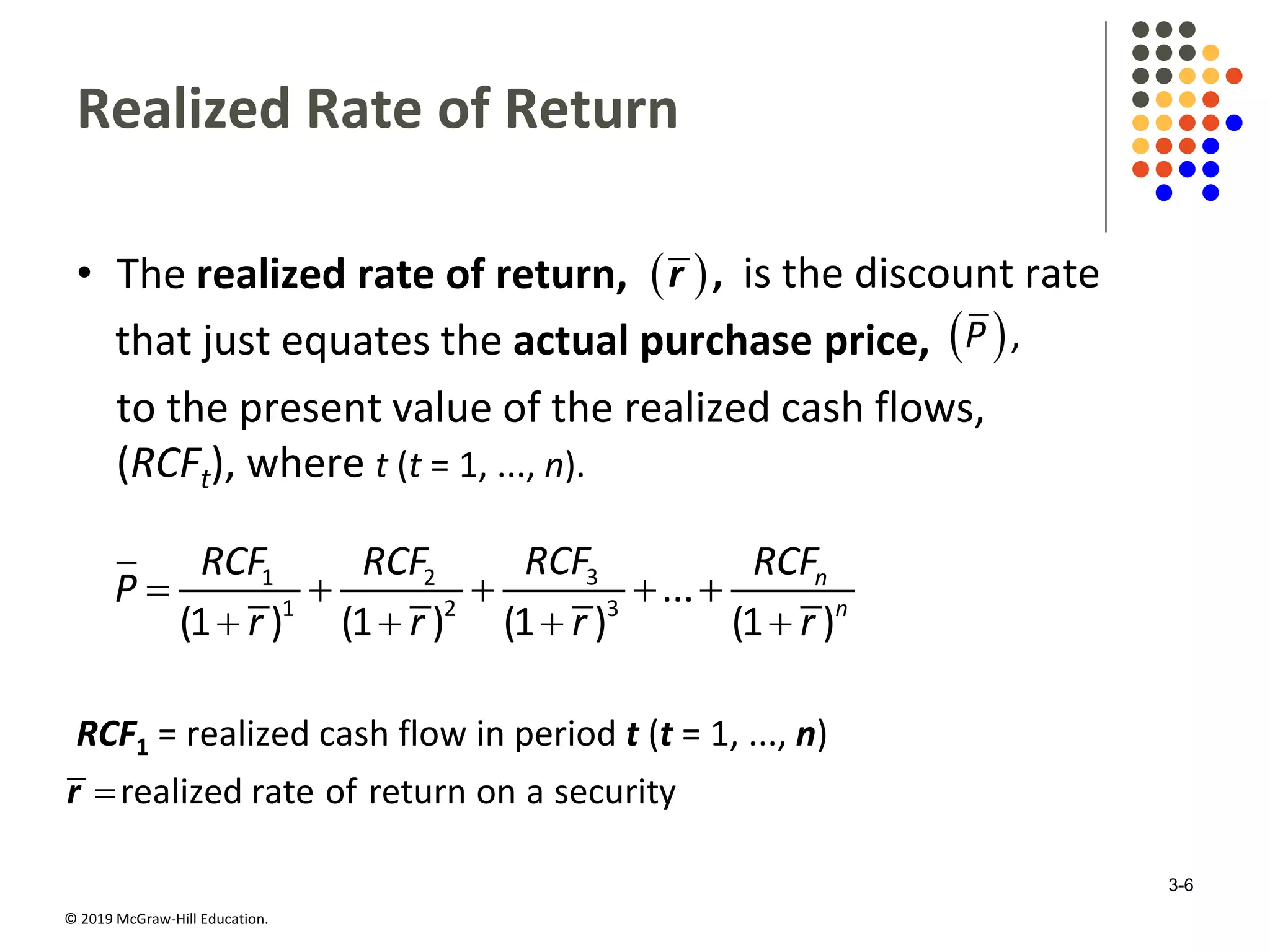
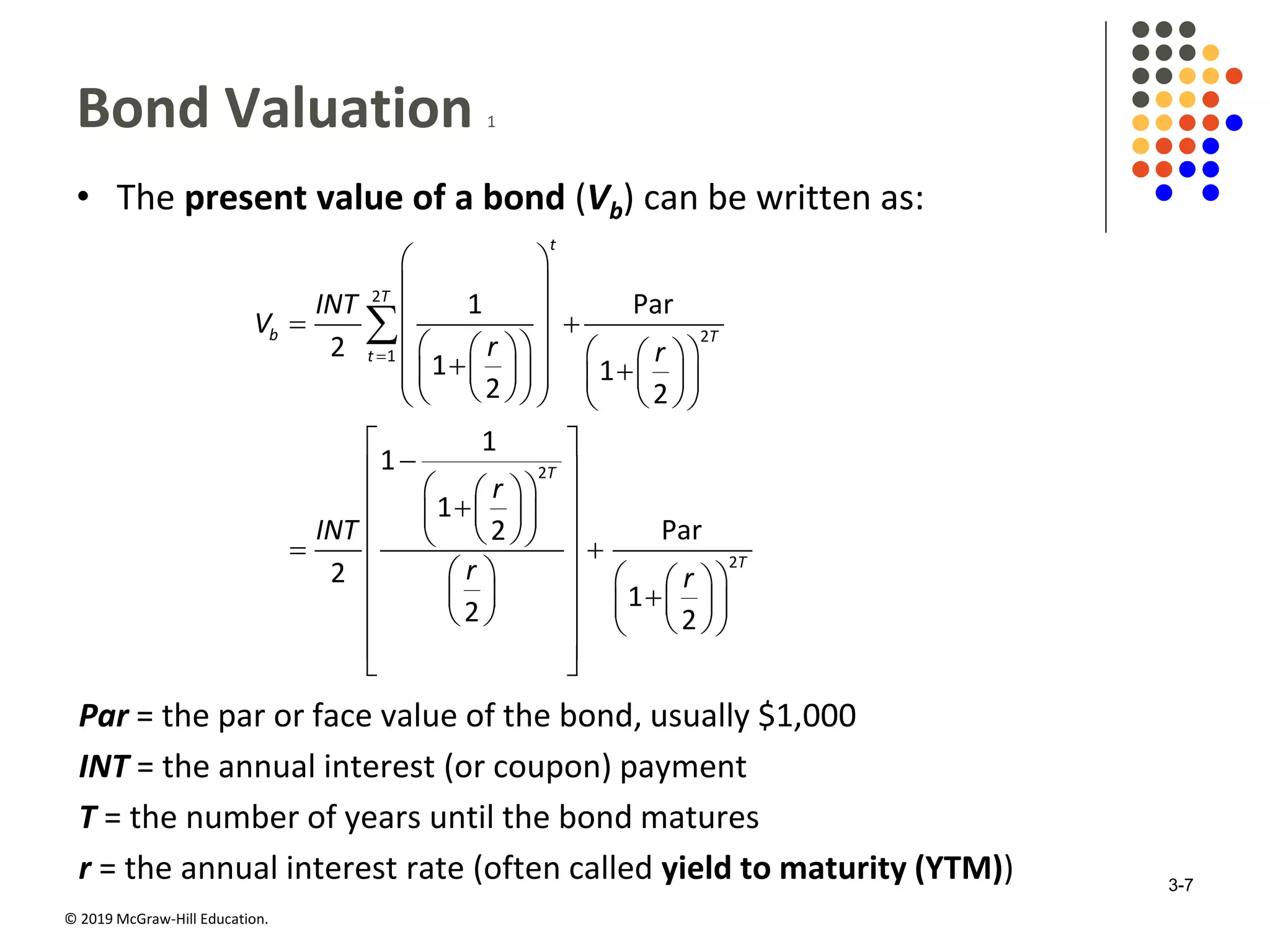
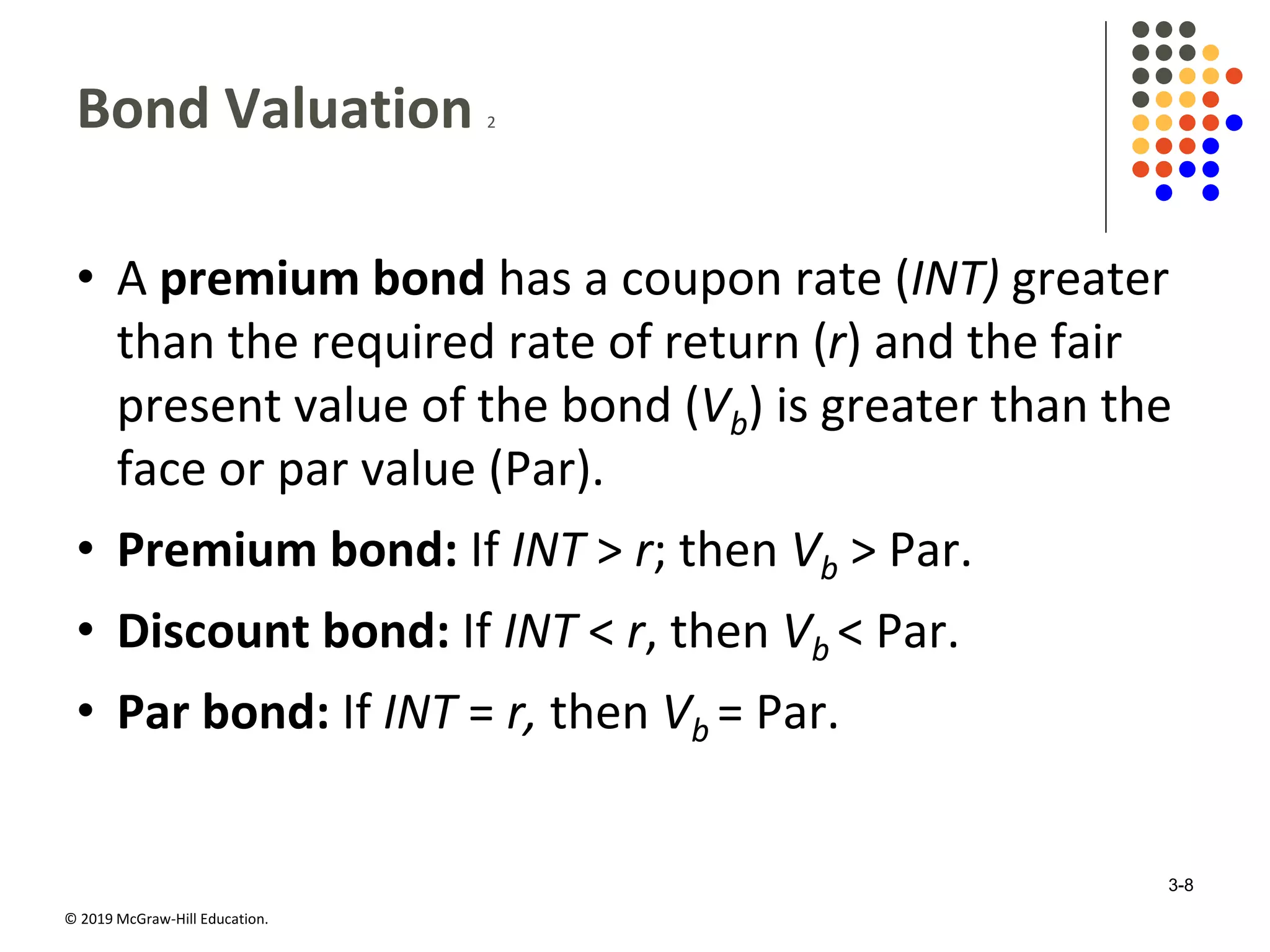
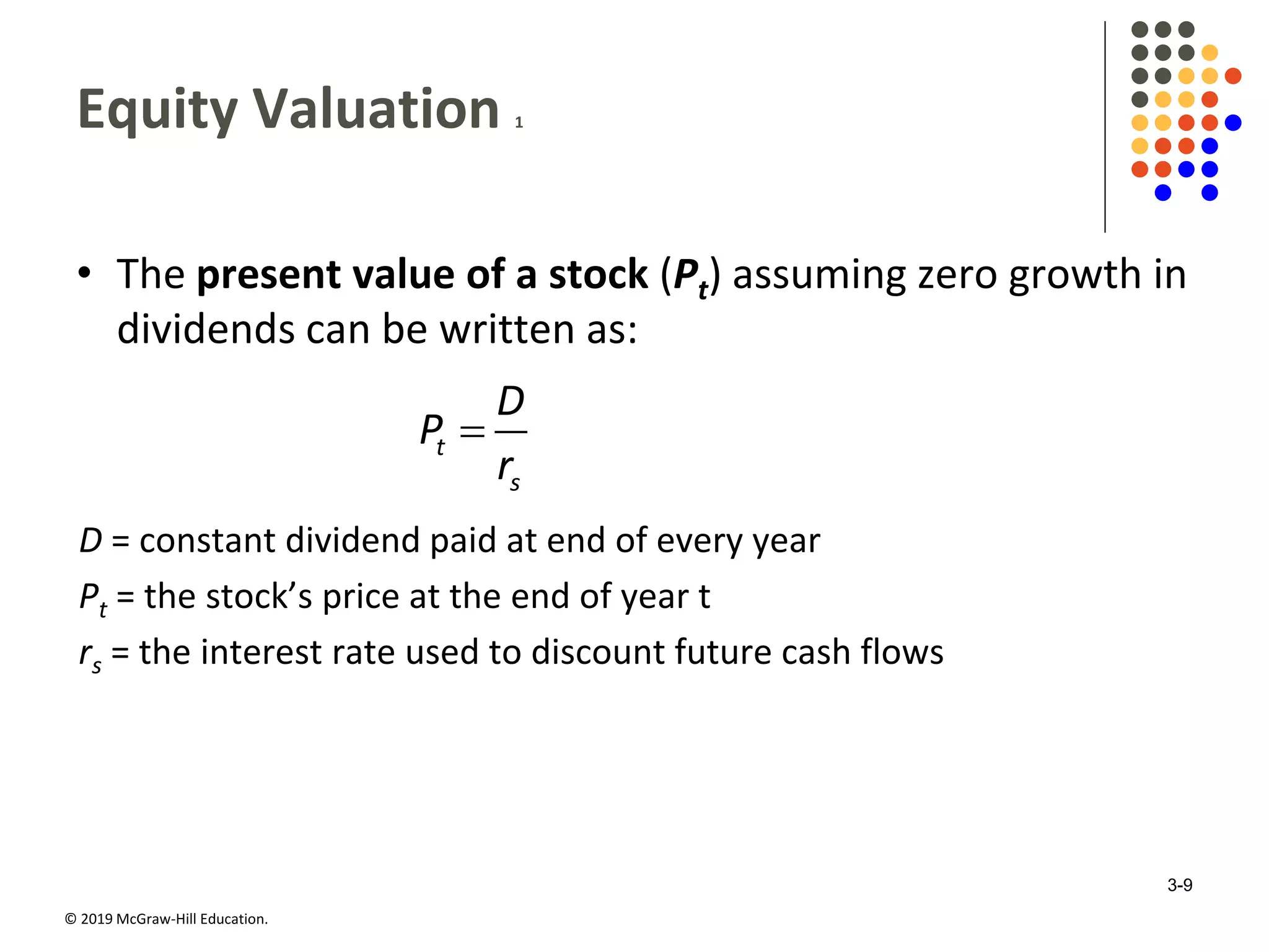
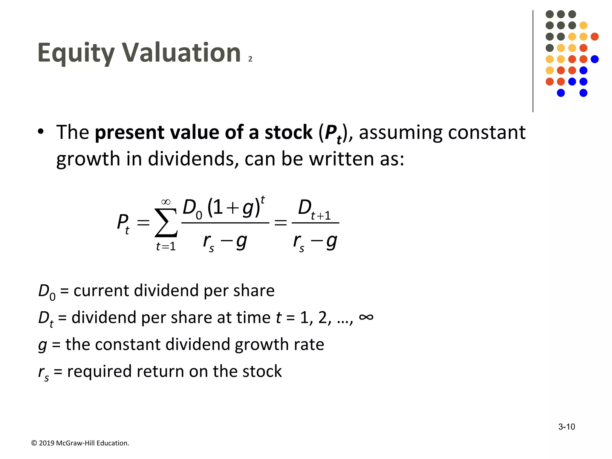
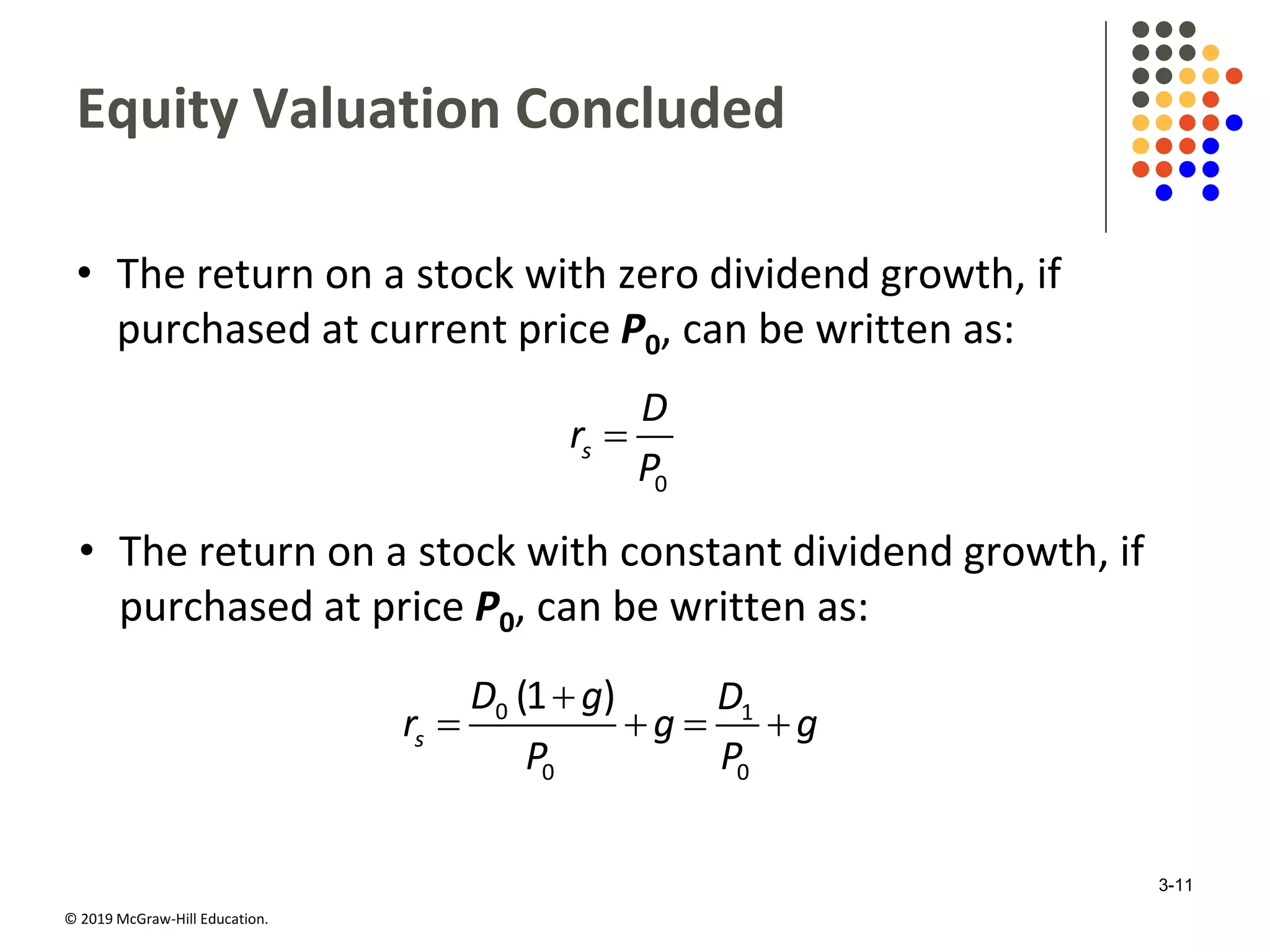
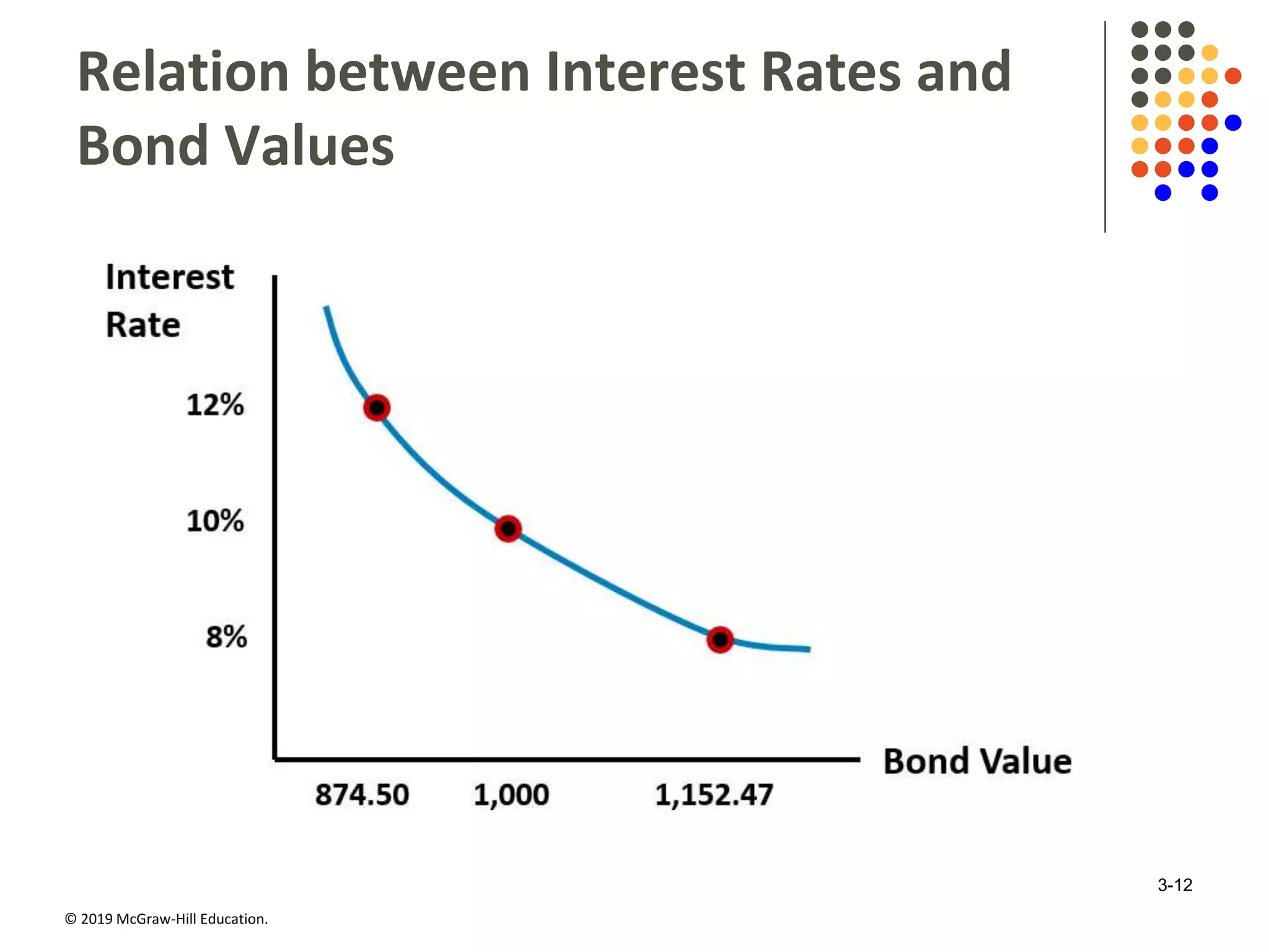
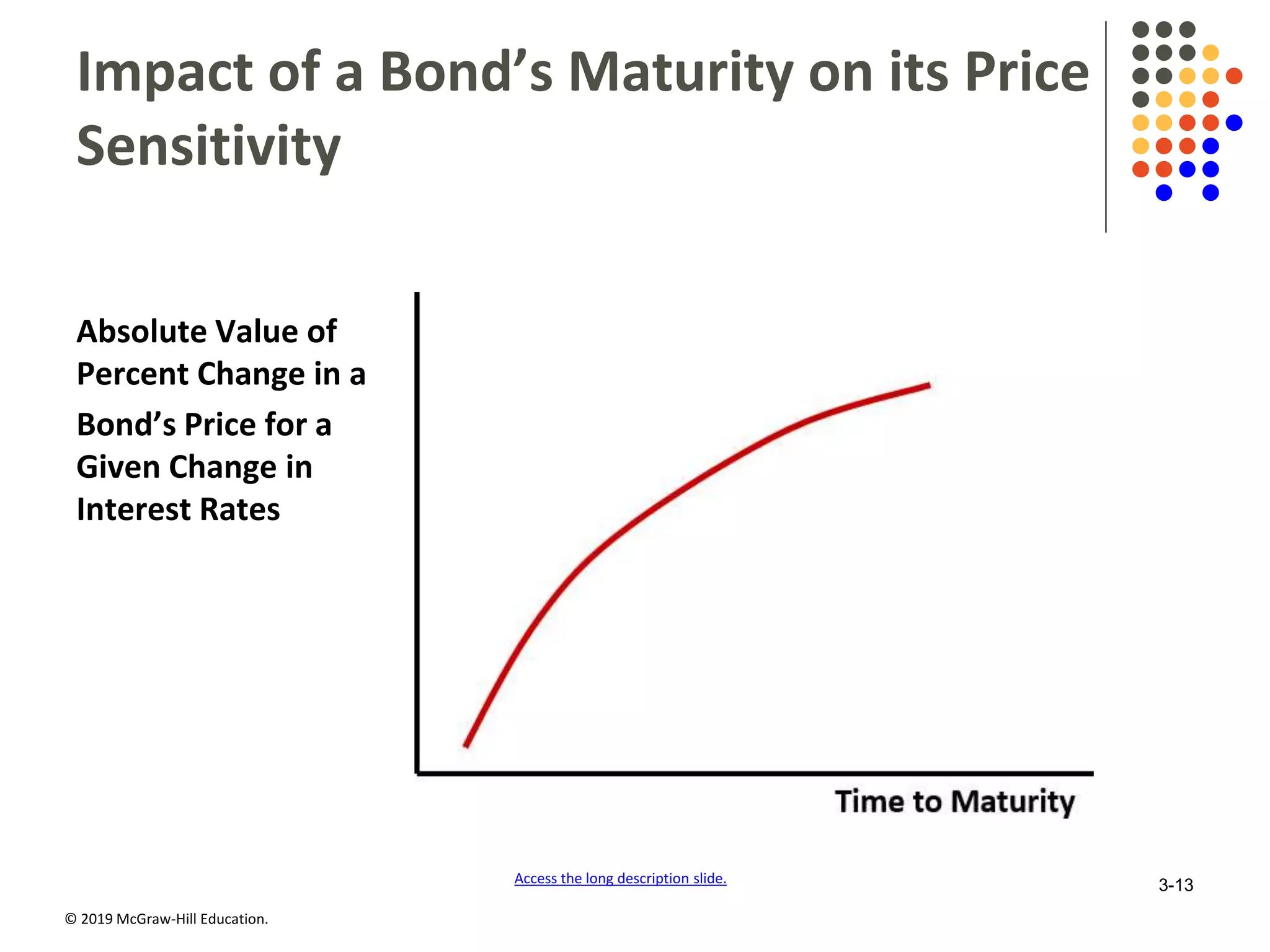
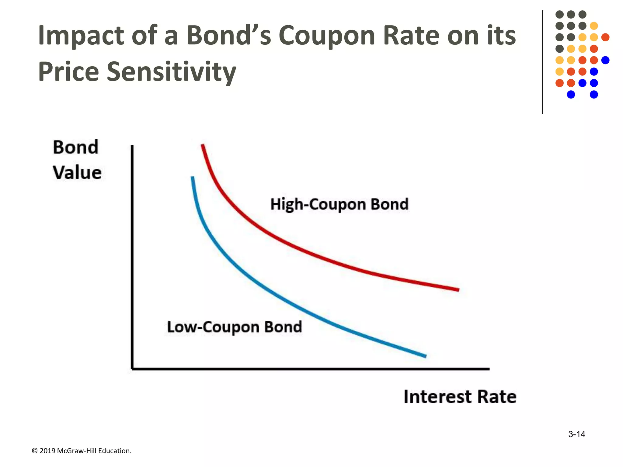
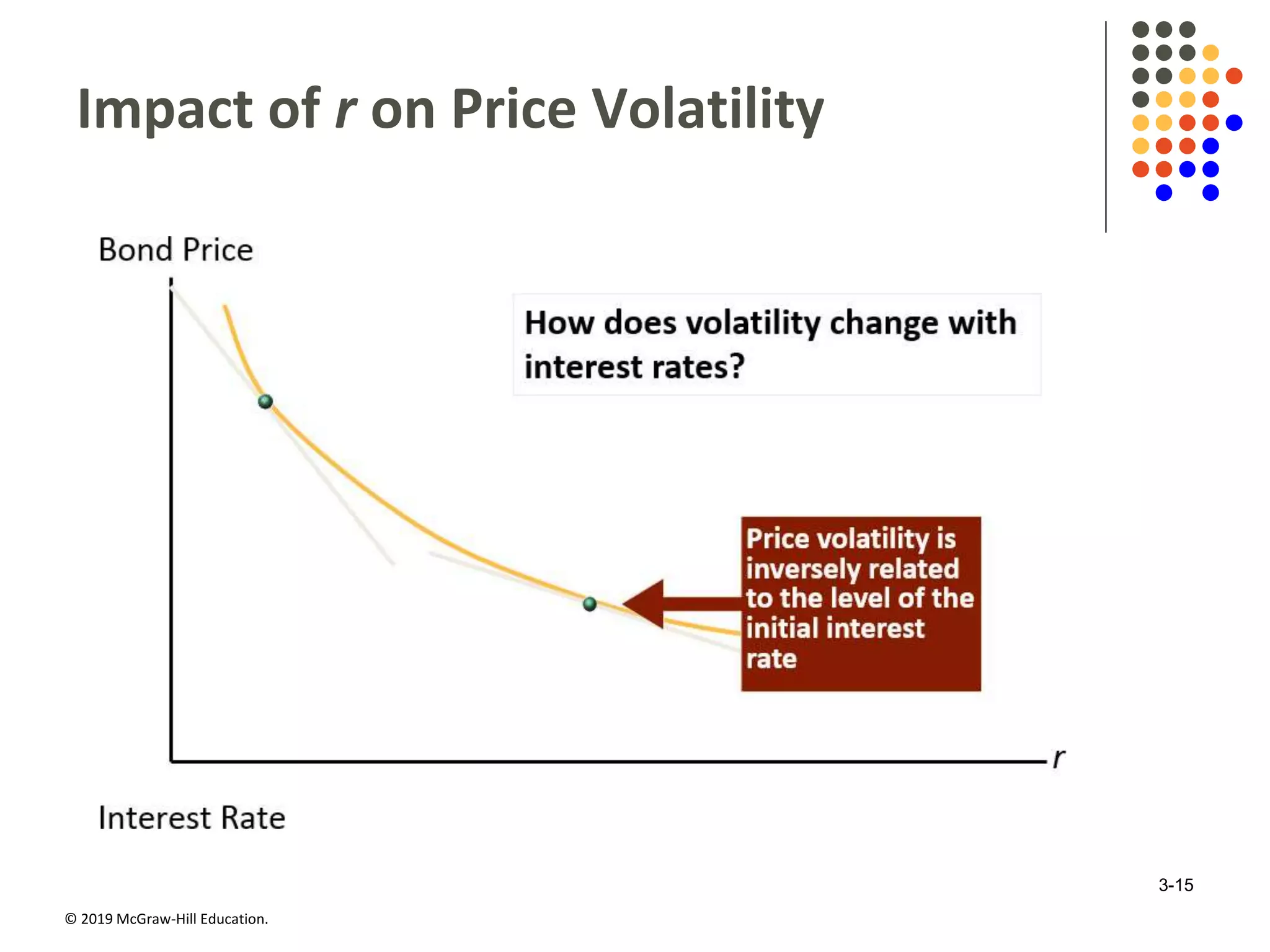
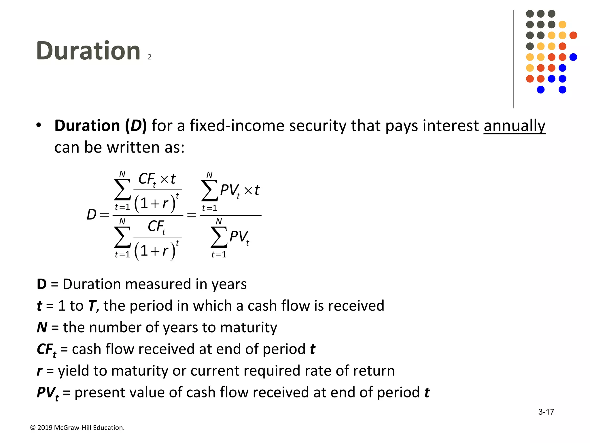
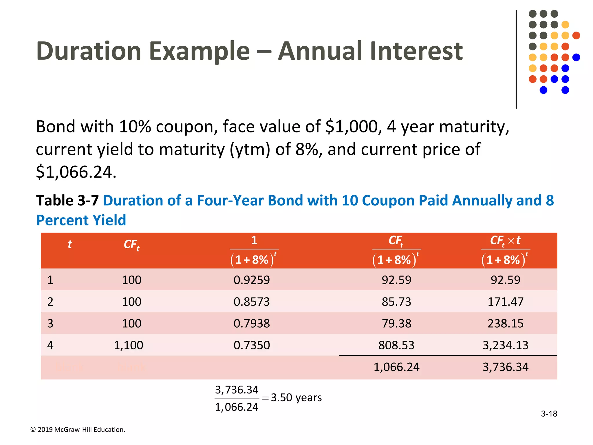
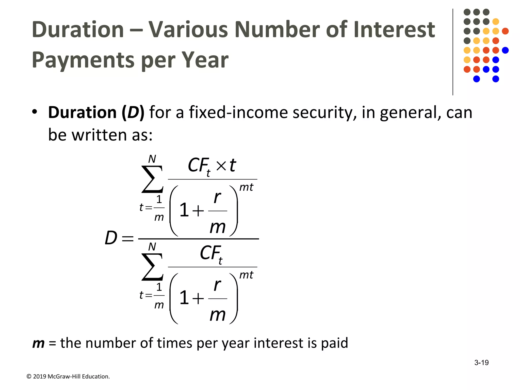
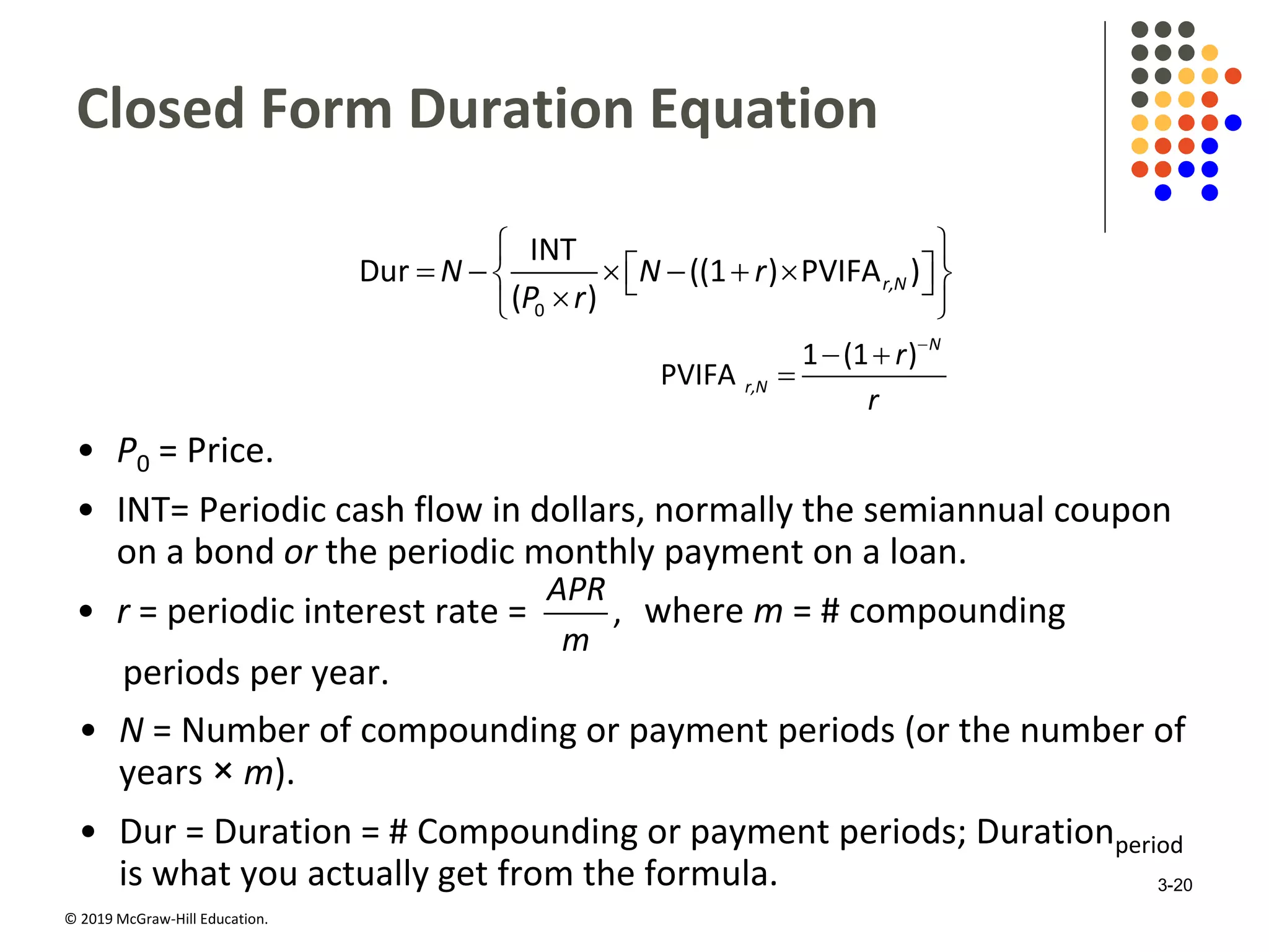
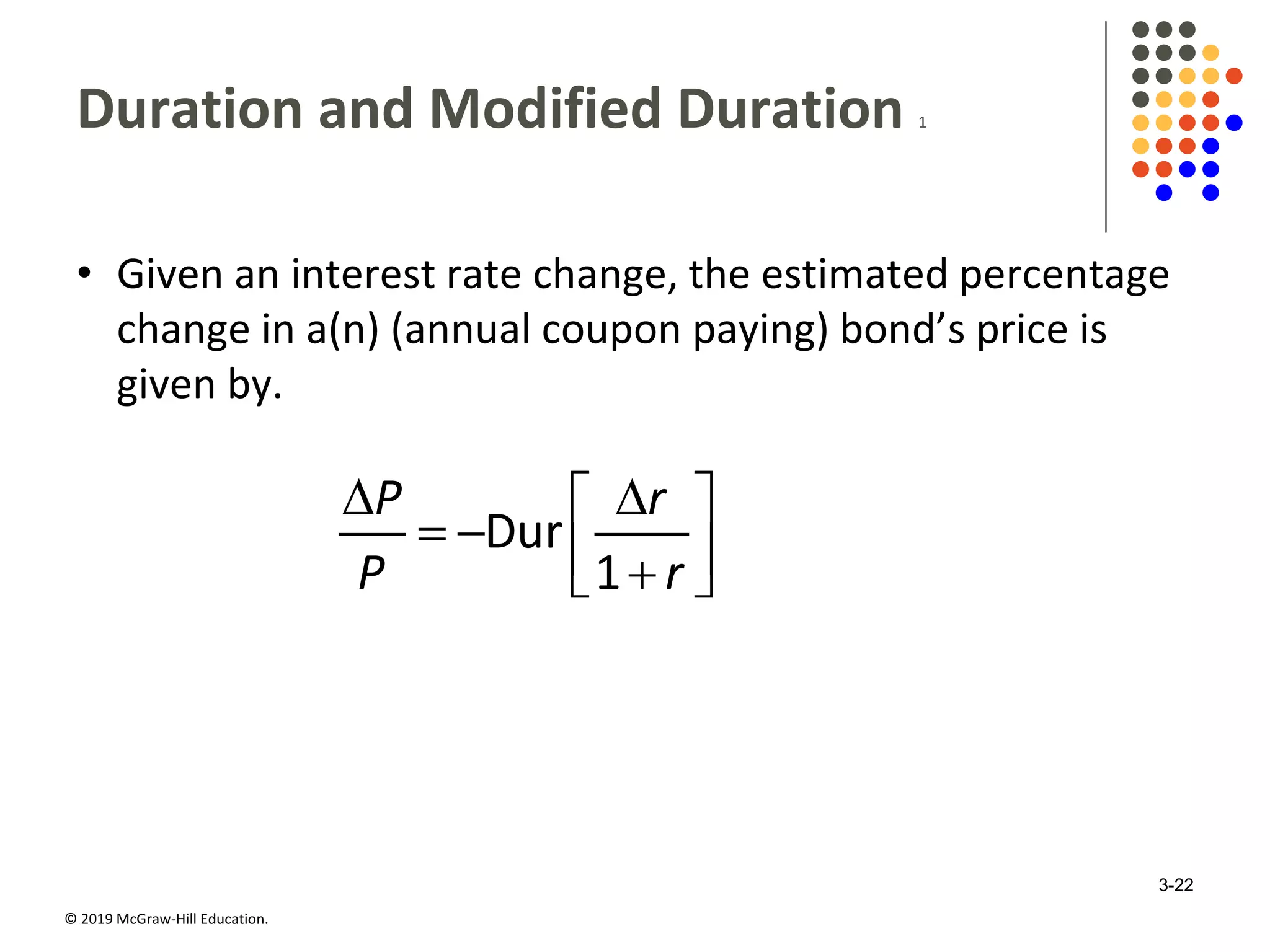
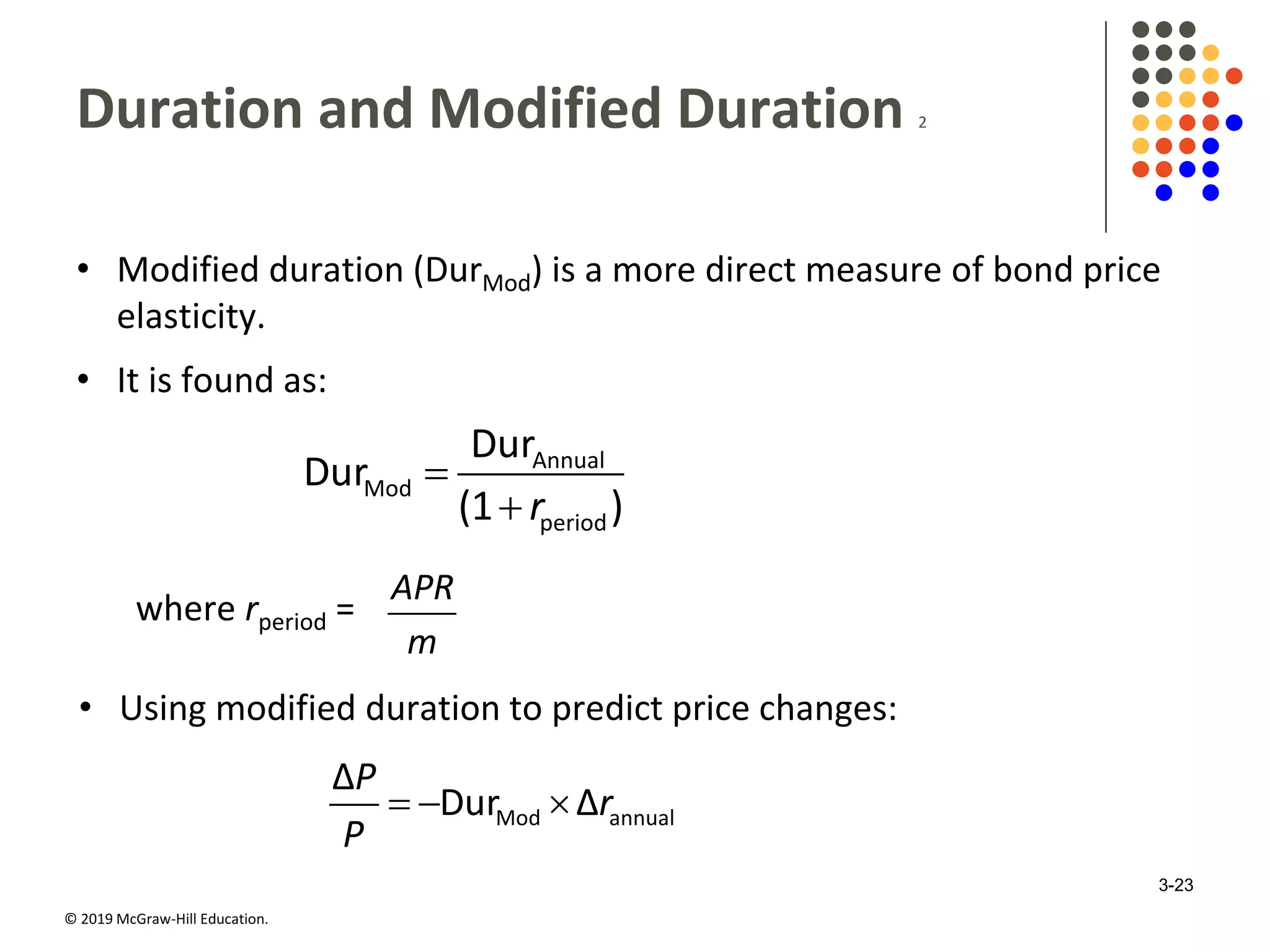
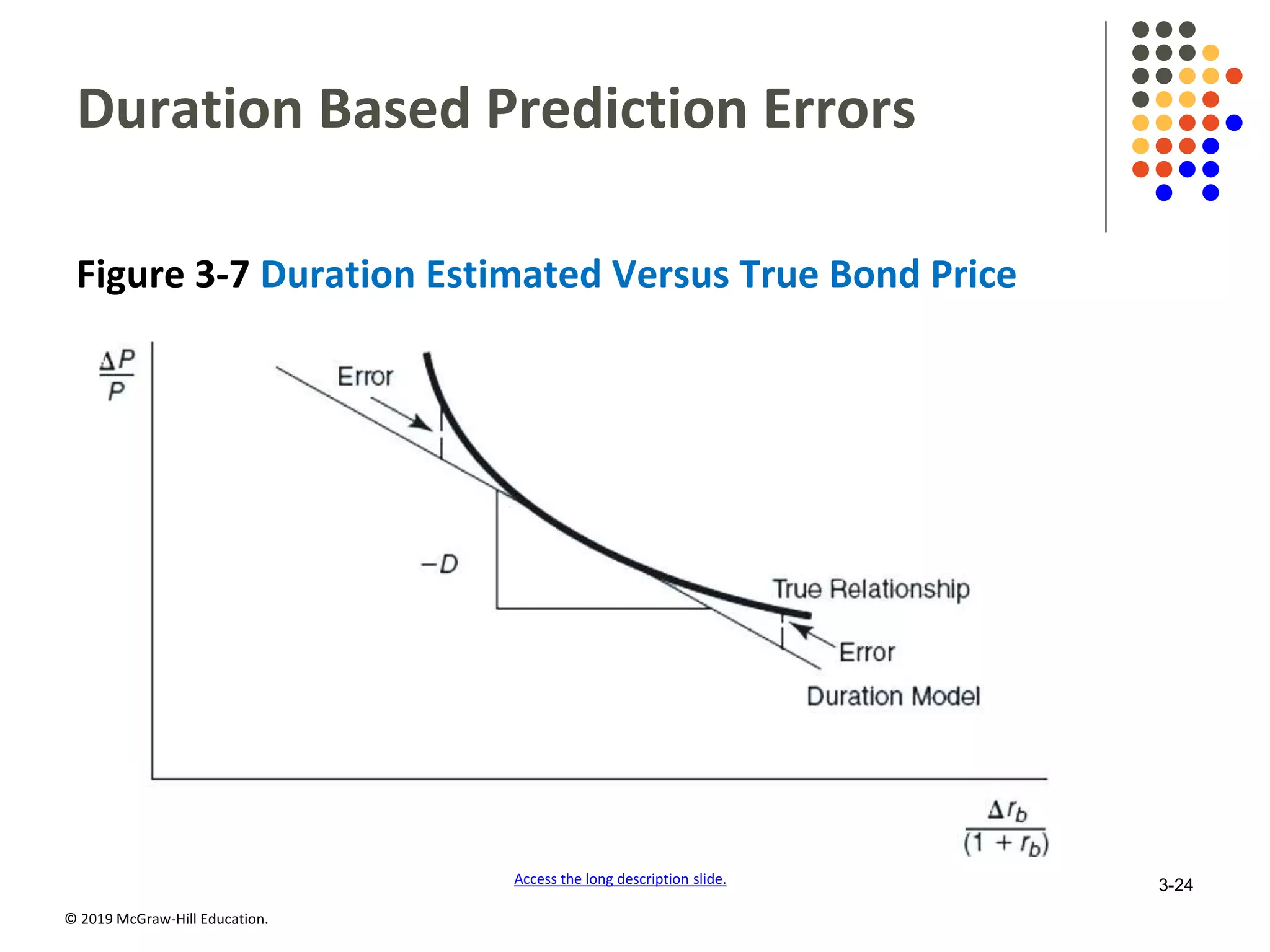
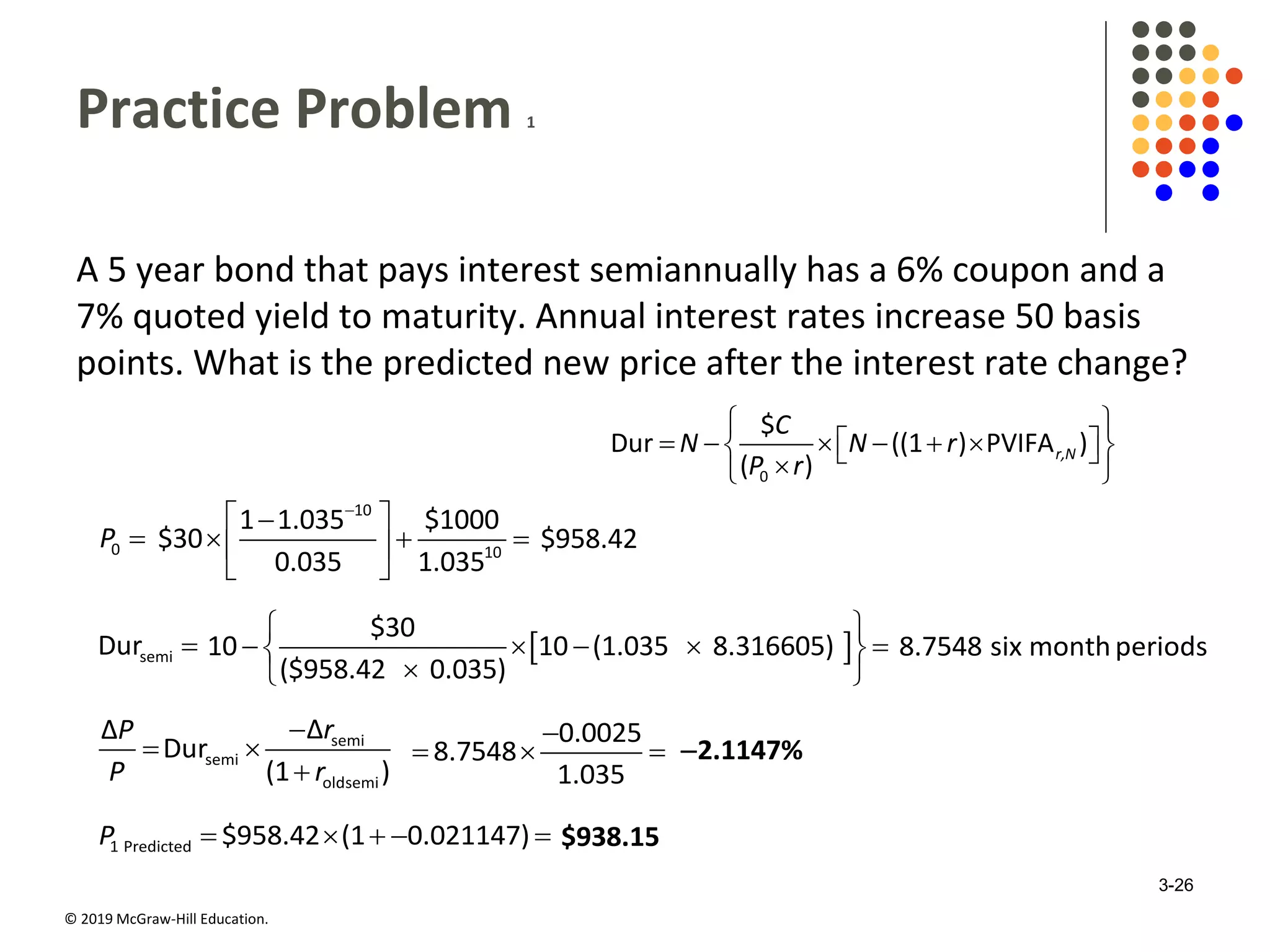
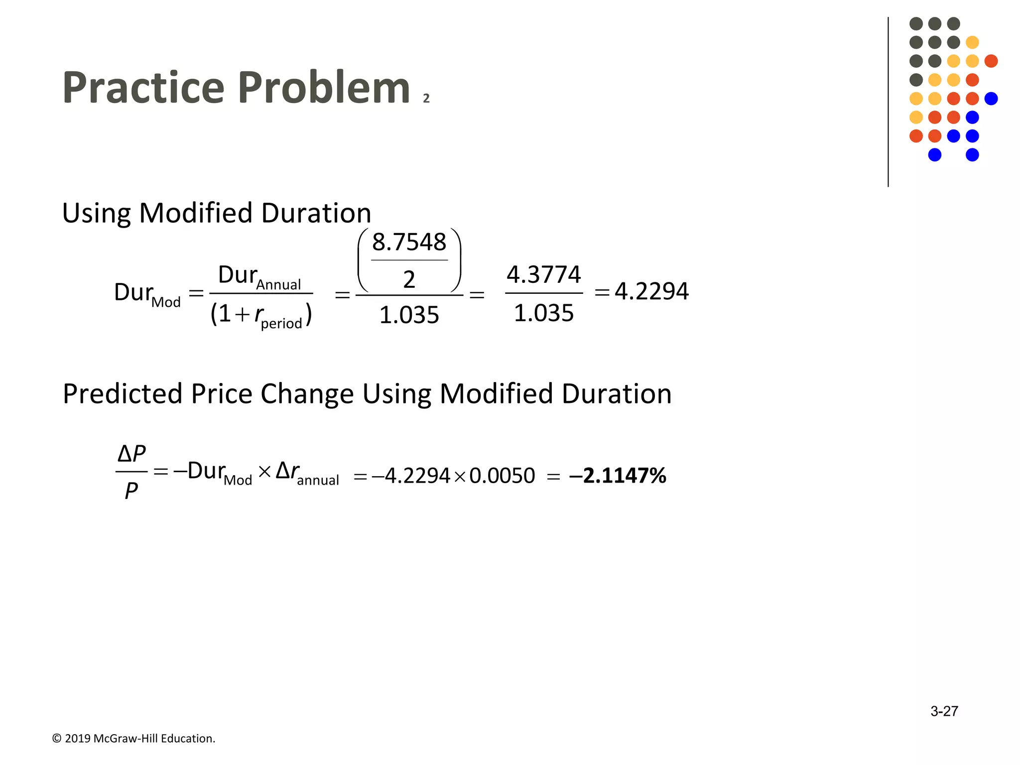
Ch. 1 1
Financial Markets
Course Code 456414
by
Dr. Muath Asmar
An-Najah National University
Faculty of Graduate Studies
Chapter Three
Interest Rates and
Security Valuation
©2019 McGraw-Hill Education. All rights reserved. Authorized only for instructor use in the classroom. No reproduction or further distribution permitted without the prior written
consent of McGraw-Hill Education.
© 2019 McGraw-Hill Education.
Various Interest Rate Measures
Coupon rate.
• periodic cash flow a bond issuer contractually promises to pay a
bond holder.
Required rate of return (r).
• rates used by individual market participants to calculate fair present
values (PV).
Expected rate of return or E(r).
• rates participants expect to earn by buying securities at current
market prices  p .
Realized rate of return (r).
• interest rate actually earned on investments.
3-3
© 2019 McGraw-Hill Education.
Required Rate of Return
• The fair present value (PV) of a security is determined
using the required rate of return (r) as the discount rate.
    
   
% % % %1 2 3
1 2 3
...
(1 ) (1 ) (1 ) (1 )
n
n
CF CF CF CF
PV
r r r r
CF1 = cash flow in period t (t = 1, …, n)
~ = indicates the projected cash flow is uncertain
n = number of periods in the investment horizon
3-4
© 2019 McGraw-Hill Education.
Expected Rate of Return
• The current market price (P) of a security is determined
using the expected rate of return, or E(r), as the discount
rate.
    
   
% % % %1 2 3
1 2 3
...
(1 ( )) (1 ( )) (1 ( )) (1 ( ))
n
n
CF CF CF CF
P
E r E r E r E r
CF1 = cash flow in period t (t = 1, …, n)
~ = indicates the projected cash flow is uncertain
n = number of periods in the investment horizon
3-5
© 2019 McGraw-Hill Education.
Realized Rate of Return
• The realized rate of return,  ,r is the discount rate
that just equates the actual purchase price,  ,P
to the present value of the realized cash flows,
(RCFt), where t (t = 1, ..., n).
31 2
1 2 3
...
(1 ) (1 ) (1 ) (1 )
n
n
RCFRCF RCF RCF
P
r r r r
    
   
RCF1 = realized cash flow in period t (t = 1, ..., n)
realized rate of return on a securityr
3-6
© 2019 McGraw-Hill Education.
Bond Valuation 1
• The present value of a bond (Vb) can be written as:

 
 
  
                   
 
 
     
                   
 
 

2
2
1
2
2
1 Par
2
1 1
2 2
1
1
1
Par2
2
1
2 2
t
T
b T
t
T
T
INT
V
r r
r
INT
r r
Par = the par or face value of the bond, usually $1,000
INT = the annual interest (or coupon) payment
T = the number of years until the bond matures
r = the annual interest rate (often called yield to maturity (YTM)) 3-7
© 2019 McGraw-Hill Education.
Bond Valuation 2
• A premium bond has a coupon rate (INT) greater
than the required rate of return (r) and the fair
present value of the bond (Vb) is greater than the
face or par value (Par).
• Premium bond: If INT > r; then Vb > Par.
• Discount bond: If INT < r, then Vb < Par.
• Par bond: If INT = r, then Vb = Par.
3-8
© 2019 McGraw-Hill Education.
Equity Valuation 1
• The present value of a stock (Pt) assuming zero growth in
dividends can be written as:
t
s
D
P
r
D = constant dividend paid at end of every year
Pt = the stock’s price at the end of year t
rs = the interest rate used to discount future cash flows
3-9
© 2019 McGraw-Hill Education.
Equity Valuation 2
• The present value of a stock (Pt), assuming constant
growth in dividends, can be written as:




 
 
 0 1
1
(1 )t
t
t
t s s
D g D
P
r g r g
D0 = current dividend per share
Dt = dividend per share at time t = 1, 2, …, ∞
g = the constant dividend growth rate
rs = required return on the stock
3-10
© 2019 McGraw-Hill Education.
Equity Valuation Concluded
• The return on a stock with zero dividend growth, if
purchased at current price P0, can be written as:

0
s
D
r
P
• The return on a stock with constant dividend growth, if
purchased at price P0, can be written as:

   0 1
0 0
(1 )
s
D g D
r g g
P P
3-11
© 2019 McGraw-Hill Education.
Relation between Interest Rates and
Bond Values
3-12
© 2019 McGraw-Hill Education.
Impact of a Bond’s Maturity on its Price
Sensitivity
Absolute Value of
Percent Change in a
Bond’s Price for a
Given Change in
Interest Rates
Access the long description slide. 3-13
© 2019 McGraw-Hill Education.
Impact of a Bond’s Coupon Rate on its
Price Sensitivity
3-14
© 2019 McGraw-Hill Education.
Impact of r on Price Volatility
3-15
© 2019 McGraw-Hill Education.
Duration 1
• Duration is the weighted-average time to
maturity (measured in years) on a financial
security.
• Duration measures the sensitivity (or elasticity)
of a fixed-income security’s price to small interest
rate changes.
• Duration captures the coupon and maturity
effects on volatility.
3-16
© 2019 McGraw-Hill Education.
Duration 2
• Duration (D) for a fixed-income security that pays interest annually
can be written as:
 
 
 
 



 

 
 
1 1
1 1
1
1
N N
t
t t
t t
N N
t
tt
t t
CF t
PV t
r
D
CF
PV
r
D = Duration measured in years
t = 1 to T, the period in which a cash flow is received
N = the number of years to maturity
CFt = cash flow received at end of period t
r = yield to maturity or current required rate of return
PVt = present value of cash flow received at end of period t
3-17
© 2019 McGraw-Hill Education.
Duration Example – Annual Interest
Bond with 10% coupon, face value of $1,000, 4 year maturity,
current yield to maturity (ytm) of 8%, and current price of
$1,066.24.
Table 3-7 Duration of a Four-Year Bond with 10 Coupon Paid Annually and 8
Percent Yield
t CFt
1 100 0.9259 92.59 92.59
2 100 0.8573 85.73 171.47
3 100 0.7938 79.38 238.15
4 1,100 0.7350 808.53 3,234.13
blank blank Blank 1,066.24 3,736.34
3,736.34
3.50 years
1,066.24

 
1
1+ 8%
t
 1+ 8%
t
t
CF
 

1+ 8%
t
t
CF t
3-18
© 2019 McGraw-Hill Education.
Duration – Various Number of Interest
Payments per Year
• Duration (D) for a fixed-income security, in general, can
be written as:



 
 
 
 
 
 


1
1
1
1
N
t
mt
t
m
N
t
mt
t
m
CF t
r
m
D
CF
r
m
m = the number of times per year interest is paid
3-19
© 2019 McGraw-Hill Education.
Closed Form Duration Equation
0
INT
Dur ((1 ) PVIFA )
( )
r,NN N r
P r
 
         
1 (1 )
PVIFA
N
r,N
r
r

 

• P0 = Price.
• INT= Periodic cash flow in dollars, normally the semiannual coupon
on a bond or the periodic monthly payment on a loan.
• r = periodic interest rate = ,
APR
m
where m = # compounding
periods per year.
• N = Number of compounding or payment periods (or the number of
years × m).
• Dur = Duration = # Compounding or payment periods; Durationperiod
is what you actually get from the formula. 3-20
© 2019 McGraw-Hill Education.
Features of Duration
Duration and coupon interest.
• The higher the coupon or promised interest payment on the bond,
the shorter its duration.
• Due to the fact that the larger the coupon or promised interest payment,
the more quickly investors receive cash flows on a bond and the higher are
the present value weights of those cash flows in the duration calculation.
Duration and rate of return.
• Duration decreases as the rate of return on the bond increases.
Duration and maturity.
• Duration increases with maturity, but at a decreasing rate
3-21
© 2019 McGraw-Hill Education.
Duration and Modified Duration 1
• Given an interest rate change, the estimated percentage
change in a(n) (annual coupon paying) bond’s price is
given by.
Dur
1
P r
P r
  
    
3-22
© 2019 McGraw-Hill Education.
Duration and Modified Duration 2
• Modified duration (DurMod) is a more direct measure of bond price
elasticity.
• It is found as:
Annual
Mod
period
Dur
Dur
(1 )r


where rperiod =
APR
m
• Using modified duration to predict price changes:
Mod annual
Δ
Dur Δ
P
r
P
  
3-23
© 2019 McGraw-Hill Education.
Duration Based Prediction Errors
Figure 3-7 Duration Estimated Versus True Bond Price
Access the long description slide. 3-24
© 2019 McGraw-Hill Education.
Convexity
Convexity (CX) is the degree of curvature of the price-
interest rate curve around some interest rate level.
• Convexity is desirable.
• The greater the convexity of a security or portfolio, the more insurance or
interest rate protection an investor or FI manager has against rate
increases and the greater the potential gains after interest rate falls.
• Convexity diminishes the error in duration as an investment
criterion.
• All fixed-income securities are convex.
• As interest rates change, bond prices change at a nonconstant rate.
3-25
© 2019 McGraw-Hill Education.
Practice Problem 1
A 5 year bond that pays interest semiannually has a 6% coupon and a
7% quoted yield to maturity. Annual interest rates increase 50 basis
points. What is the predicted new price after the interest rate change?
0
$
Dur ((1 ) PVIFA )
( )
r,N
C
N N r
P r
 
         
0P 
10
10
1 1.035 $1000
$30
0.035 1.035

 
   
 
$958.42
semiDur   
$30
10 10 (1.035 8.316605)
($958.42 0.035)
 
     
 
8.7548 six monthperiods
semi
semi
oldsemi
ΔΔ
Dur
(1 )
rP
P r

 

0.0025
8.7548
1.035

   2.1147%
1 Predicted $958.42 (1 0.021147)P      $938.15
3-26
© 2019 McGraw-Hill Education.
Practice Problem 2
Using Modified Duration
Annual
Mod
period
Dur
Dur
(1 )r


 
 
  
8.7548
2
1.035
4.3774
1.035
4.2294
Predicted Price Change Using Modified Duration
Mod annual
Δ
Dur Δ
P
r
P
   4.2294 0.0050    2.1147%
3-27
© 2019 McGraw-Hill Education.
Impact of a Bond’s Maturity on its Price
Sensitivity Long Description
Line graph showing that as time to maturity increases
the absolute value of the percentage change in a
bond's price for a given change in interest rate
increases in a nonlinear, concave down manner.
Return to slide containing original image. 3-28
© 2019 McGraw-Hill Education.
Duration Based Prediction Errors Long
Description
The true relationship is vertically greater than the
duration model, but the duration model lies tangent to
this curve. The vertical distance between the duration
model and the true relationship is labeled error.
Return to slide containing original image. 3-29

Chapter (3)

  • 1.
    Ch. 1 1 FinancialMarkets Course Code 456414 by Dr. Muath Asmar An-Najah National University Faculty of Graduate Studies
  • 2.
    Chapter Three Interest Ratesand Security Valuation ©2019 McGraw-Hill Education. All rights reserved. Authorized only for instructor use in the classroom. No reproduction or further distribution permitted without the prior written consent of McGraw-Hill Education.
  • 3.
    © 2019 McGraw-HillEducation. Various Interest Rate Measures Coupon rate. • periodic cash flow a bond issuer contractually promises to pay a bond holder. Required rate of return (r). • rates used by individual market participants to calculate fair present values (PV). Expected rate of return or E(r). • rates participants expect to earn by buying securities at current market prices  p . Realized rate of return (r). • interest rate actually earned on investments. 3-3
  • 4.
    © 2019 McGraw-HillEducation. Required Rate of Return • The fair present value (PV) of a security is determined using the required rate of return (r) as the discount rate.          % % % %1 2 3 1 2 3 ... (1 ) (1 ) (1 ) (1 ) n n CF CF CF CF PV r r r r CF1 = cash flow in period t (t = 1, …, n) ~ = indicates the projected cash flow is uncertain n = number of periods in the investment horizon 3-4
  • 5.
    © 2019 McGraw-HillEducation. Expected Rate of Return • The current market price (P) of a security is determined using the expected rate of return, or E(r), as the discount rate.          % % % %1 2 3 1 2 3 ... (1 ( )) (1 ( )) (1 ( )) (1 ( )) n n CF CF CF CF P E r E r E r E r CF1 = cash flow in period t (t = 1, …, n) ~ = indicates the projected cash flow is uncertain n = number of periods in the investment horizon 3-5
  • 6.
    © 2019 McGraw-HillEducation. Realized Rate of Return • The realized rate of return,  ,r is the discount rate that just equates the actual purchase price,  ,P to the present value of the realized cash flows, (RCFt), where t (t = 1, ..., n). 31 2 1 2 3 ... (1 ) (1 ) (1 ) (1 ) n n RCFRCF RCF RCF P r r r r          RCF1 = realized cash flow in period t (t = 1, ..., n) realized rate of return on a securityr 3-6
  • 7.
    © 2019 McGraw-HillEducation. Bond Valuation 1 • The present value of a bond (Vb) can be written as:                                                                2 2 1 2 2 1 Par 2 1 1 2 2 1 1 1 Par2 2 1 2 2 t T b T t T T INT V r r r INT r r Par = the par or face value of the bond, usually $1,000 INT = the annual interest (or coupon) payment T = the number of years until the bond matures r = the annual interest rate (often called yield to maturity (YTM)) 3-7
  • 8.
    © 2019 McGraw-HillEducation. Bond Valuation 2 • A premium bond has a coupon rate (INT) greater than the required rate of return (r) and the fair present value of the bond (Vb) is greater than the face or par value (Par). • Premium bond: If INT > r; then Vb > Par. • Discount bond: If INT < r, then Vb < Par. • Par bond: If INT = r, then Vb = Par. 3-8
  • 9.
    © 2019 McGraw-HillEducation. Equity Valuation 1 • The present value of a stock (Pt) assuming zero growth in dividends can be written as: t s D P r D = constant dividend paid at end of every year Pt = the stock’s price at the end of year t rs = the interest rate used to discount future cash flows 3-9
  • 10.
    © 2019 McGraw-HillEducation. Equity Valuation 2 • The present value of a stock (Pt), assuming constant growth in dividends, can be written as:          0 1 1 (1 )t t t t s s D g D P r g r g D0 = current dividend per share Dt = dividend per share at time t = 1, 2, …, ∞ g = the constant dividend growth rate rs = required return on the stock 3-10
  • 11.
    © 2019 McGraw-HillEducation. Equity Valuation Concluded • The return on a stock with zero dividend growth, if purchased at current price P0, can be written as:  0 s D r P • The return on a stock with constant dividend growth, if purchased at price P0, can be written as:     0 1 0 0 (1 ) s D g D r g g P P 3-11
  • 12.
    © 2019 McGraw-HillEducation. Relation between Interest Rates and Bond Values 3-12
  • 13.
    © 2019 McGraw-HillEducation. Impact of a Bond’s Maturity on its Price Sensitivity Absolute Value of Percent Change in a Bond’s Price for a Given Change in Interest Rates Access the long description slide. 3-13
  • 14.
    © 2019 McGraw-HillEducation. Impact of a Bond’s Coupon Rate on its Price Sensitivity 3-14
  • 15.
    © 2019 McGraw-HillEducation. Impact of r on Price Volatility 3-15
  • 16.
    © 2019 McGraw-HillEducation. Duration 1 • Duration is the weighted-average time to maturity (measured in years) on a financial security. • Duration measures the sensitivity (or elasticity) of a fixed-income security’s price to small interest rate changes. • Duration captures the coupon and maturity effects on volatility. 3-16
  • 17.
    © 2019 McGraw-HillEducation. Duration 2 • Duration (D) for a fixed-income security that pays interest annually can be written as:                   1 1 1 1 1 1 N N t t t t t N N t tt t t CF t PV t r D CF PV r D = Duration measured in years t = 1 to T, the period in which a cash flow is received N = the number of years to maturity CFt = cash flow received at end of period t r = yield to maturity or current required rate of return PVt = present value of cash flow received at end of period t 3-17
  • 18.
    © 2019 McGraw-HillEducation. Duration Example – Annual Interest Bond with 10% coupon, face value of $1,000, 4 year maturity, current yield to maturity (ytm) of 8%, and current price of $1,066.24. Table 3-7 Duration of a Four-Year Bond with 10 Coupon Paid Annually and 8 Percent Yield t CFt 1 100 0.9259 92.59 92.59 2 100 0.8573 85.73 171.47 3 100 0.7938 79.38 238.15 4 1,100 0.7350 808.53 3,234.13 blank blank Blank 1,066.24 3,736.34 3,736.34 3.50 years 1,066.24    1 1+ 8% t  1+ 8% t t CF    1+ 8% t t CF t 3-18
  • 19.
    © 2019 McGraw-HillEducation. Duration – Various Number of Interest Payments per Year • Duration (D) for a fixed-income security, in general, can be written as:                  1 1 1 1 N t mt t m N t mt t m CF t r m D CF r m m = the number of times per year interest is paid 3-19
  • 20.
    © 2019 McGraw-HillEducation. Closed Form Duration Equation 0 INT Dur ((1 ) PVIFA ) ( ) r,NN N r P r             1 (1 ) PVIFA N r,N r r     • P0 = Price. • INT= Periodic cash flow in dollars, normally the semiannual coupon on a bond or the periodic monthly payment on a loan. • r = periodic interest rate = , APR m where m = # compounding periods per year. • N = Number of compounding or payment periods (or the number of years × m). • Dur = Duration = # Compounding or payment periods; Durationperiod is what you actually get from the formula. 3-20
  • 21.
    © 2019 McGraw-HillEducation. Features of Duration Duration and coupon interest. • The higher the coupon or promised interest payment on the bond, the shorter its duration. • Due to the fact that the larger the coupon or promised interest payment, the more quickly investors receive cash flows on a bond and the higher are the present value weights of those cash flows in the duration calculation. Duration and rate of return. • Duration decreases as the rate of return on the bond increases. Duration and maturity. • Duration increases with maturity, but at a decreasing rate 3-21
  • 22.
    © 2019 McGraw-HillEducation. Duration and Modified Duration 1 • Given an interest rate change, the estimated percentage change in a(n) (annual coupon paying) bond’s price is given by. Dur 1 P r P r         3-22
  • 23.
    © 2019 McGraw-HillEducation. Duration and Modified Duration 2 • Modified duration (DurMod) is a more direct measure of bond price elasticity. • It is found as: Annual Mod period Dur Dur (1 )r   where rperiod = APR m • Using modified duration to predict price changes: Mod annual Δ Dur Δ P r P    3-23
  • 24.
    © 2019 McGraw-HillEducation. Duration Based Prediction Errors Figure 3-7 Duration Estimated Versus True Bond Price Access the long description slide. 3-24
  • 25.
    © 2019 McGraw-HillEducation. Convexity Convexity (CX) is the degree of curvature of the price- interest rate curve around some interest rate level. • Convexity is desirable. • The greater the convexity of a security or portfolio, the more insurance or interest rate protection an investor or FI manager has against rate increases and the greater the potential gains after interest rate falls. • Convexity diminishes the error in duration as an investment criterion. • All fixed-income securities are convex. • As interest rates change, bond prices change at a nonconstant rate. 3-25
  • 26.
    © 2019 McGraw-HillEducation. Practice Problem 1 A 5 year bond that pays interest semiannually has a 6% coupon and a 7% quoted yield to maturity. Annual interest rates increase 50 basis points. What is the predicted new price after the interest rate change? 0 $ Dur ((1 ) PVIFA ) ( ) r,N C N N r P r             0P  10 10 1 1.035 $1000 $30 0.035 1.035          $958.42 semiDur    $30 10 10 (1.035 8.316605) ($958.42 0.035)           8.7548 six monthperiods semi semi oldsemi ΔΔ Dur (1 ) rP P r     0.0025 8.7548 1.035     2.1147% 1 Predicted $958.42 (1 0.021147)P      $938.15 3-26
  • 27.
    © 2019 McGraw-HillEducation. Practice Problem 2 Using Modified Duration Annual Mod period Dur Dur (1 )r          8.7548 2 1.035 4.3774 1.035 4.2294 Predicted Price Change Using Modified Duration Mod annual Δ Dur Δ P r P    4.2294 0.0050    2.1147% 3-27
  • 28.
    © 2019 McGraw-HillEducation. Impact of a Bond’s Maturity on its Price Sensitivity Long Description Line graph showing that as time to maturity increases the absolute value of the percentage change in a bond's price for a given change in interest rate increases in a nonlinear, concave down manner. Return to slide containing original image. 3-28
  • 29.
    © 2019 McGraw-HillEducation. Duration Based Prediction Errors Long Description The true relationship is vertically greater than the duration model, but the duration model lies tangent to this curve. The vertical distance between the duration model and the true relationship is labeled error. Return to slide containing original image. 3-29