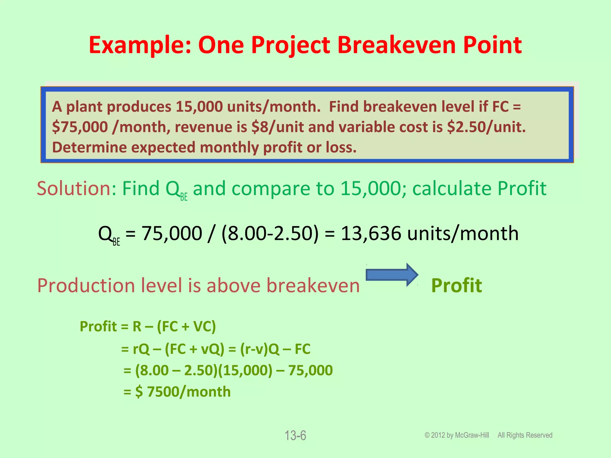
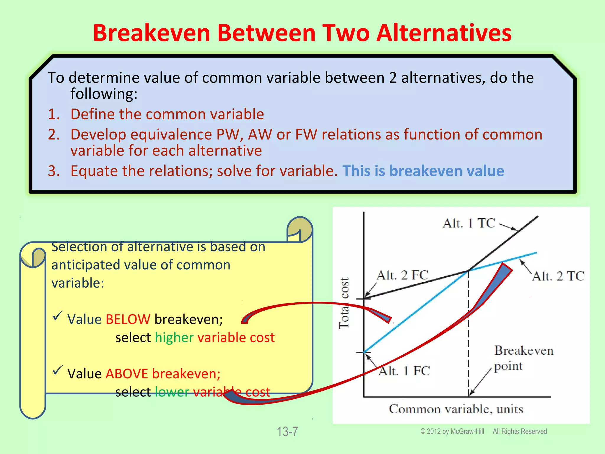
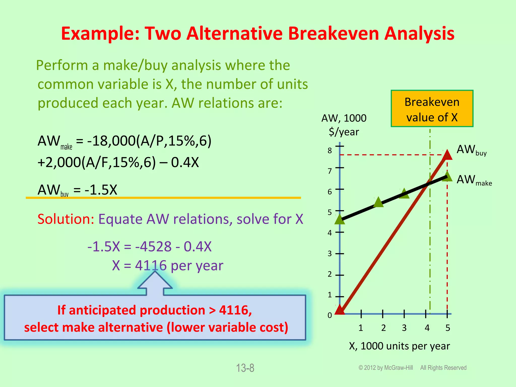
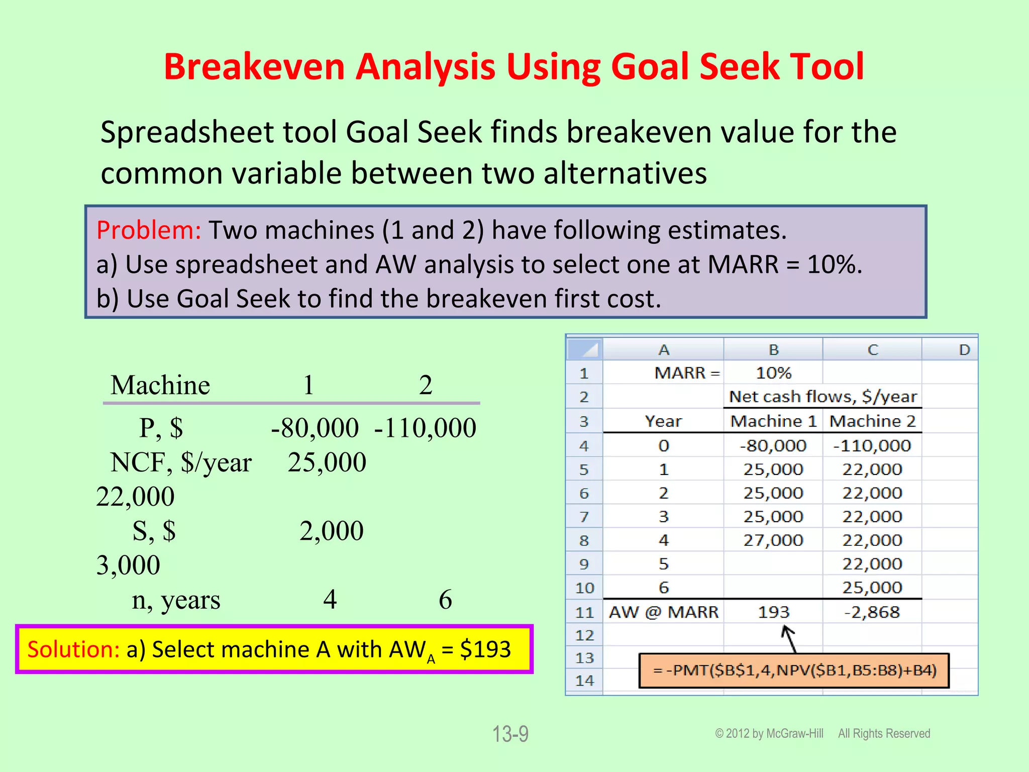
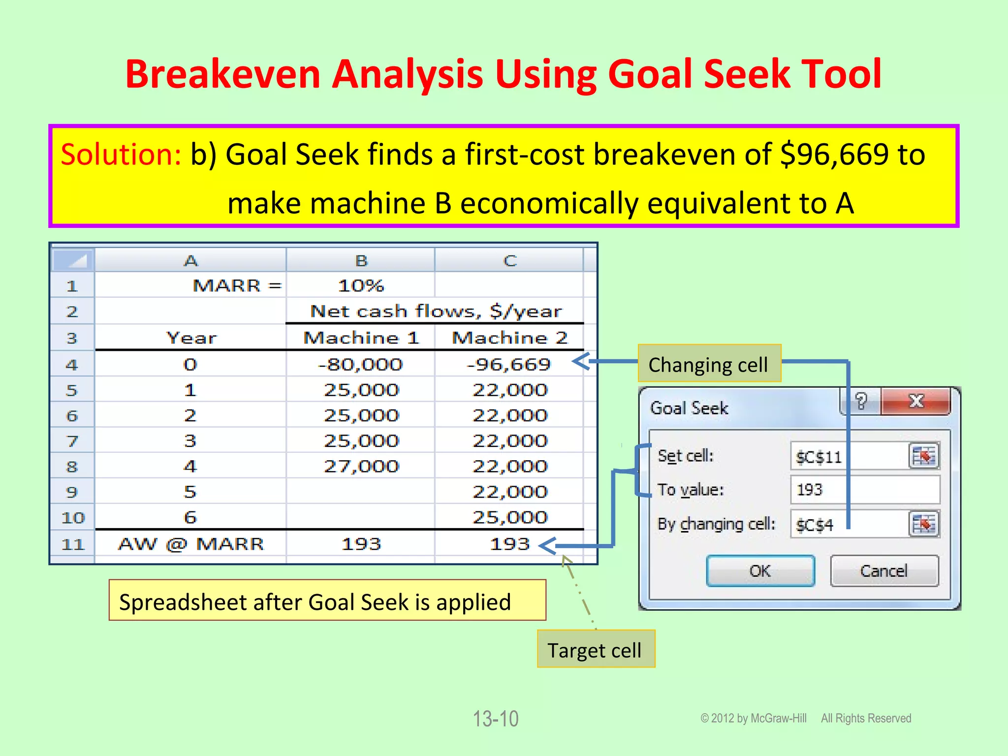
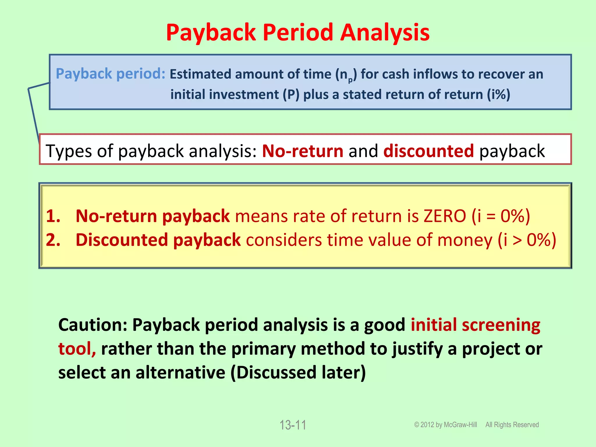
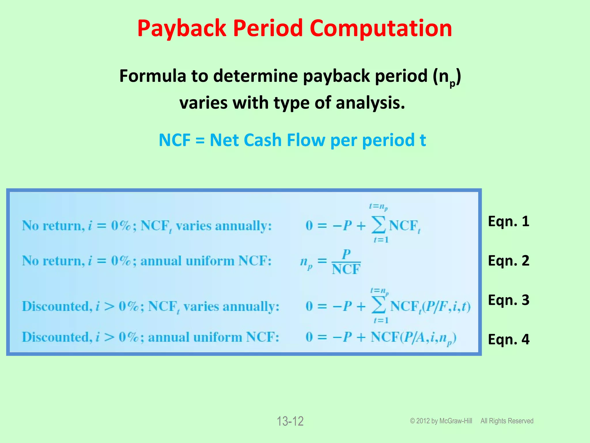
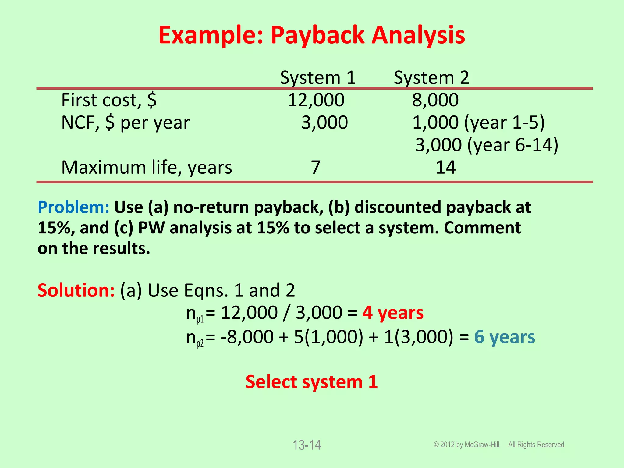
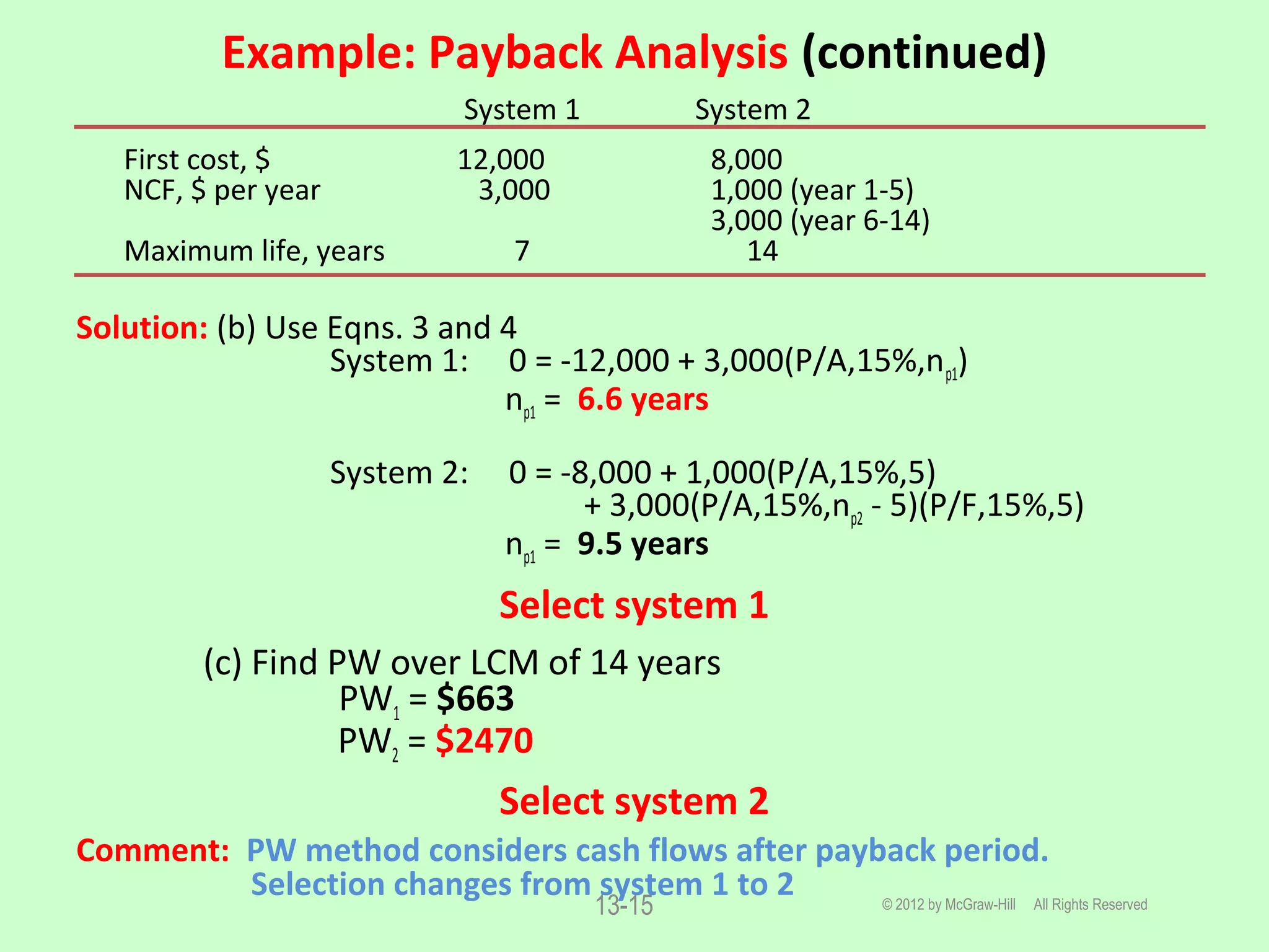
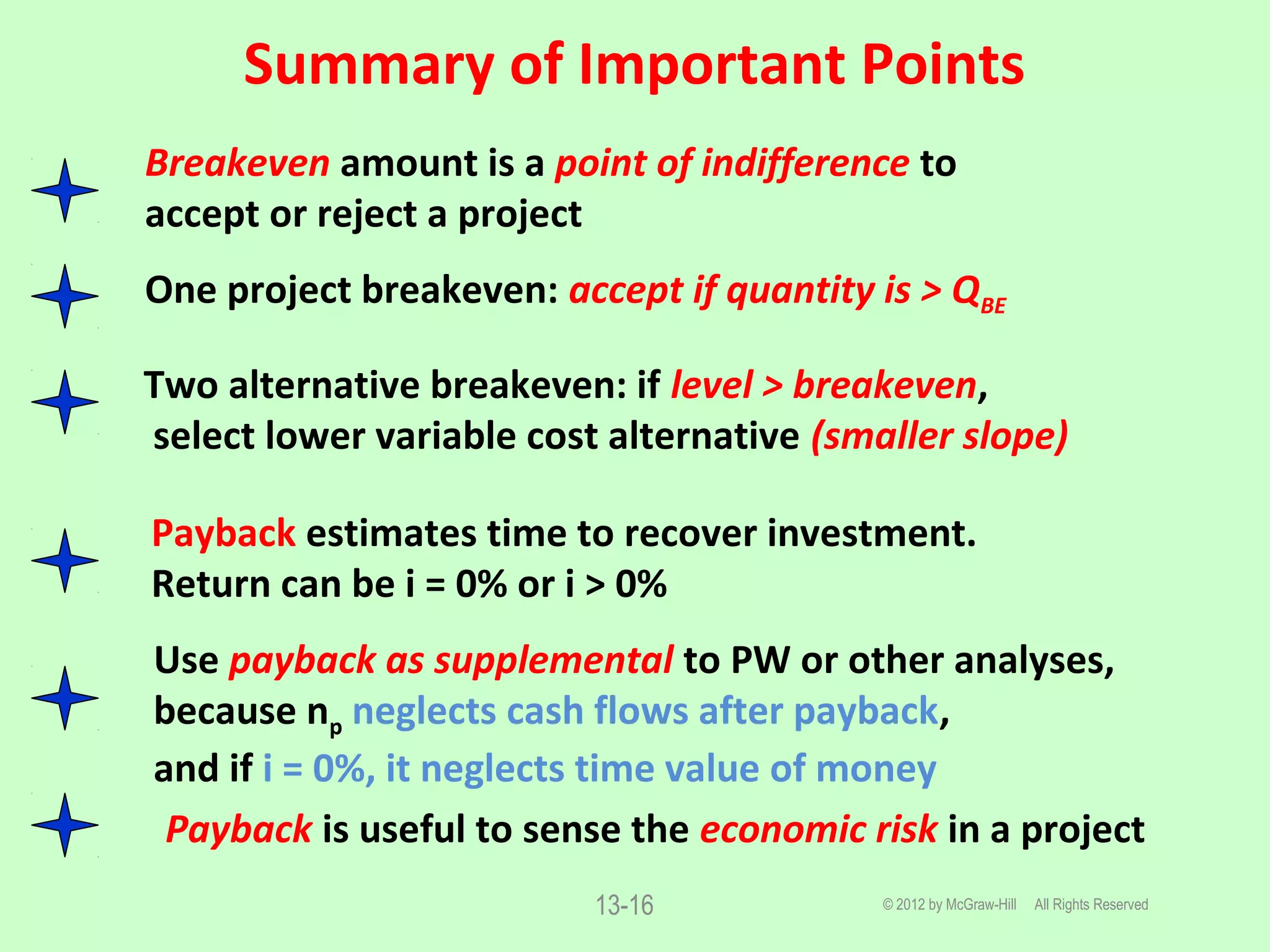
1. Breakeven analysis determines the level of a variable (e.g. quantity, units) that results in no profit or loss. It is used to evaluate a single project or choose between two alternatives. 2. Payback period is the estimated time for a project's cash inflows to recover its initial investment. It can be calculated with or without considering the time value of money (discounted vs no-return payback). 3. Both breakeven analysis and payback period are useful initial screening tools but should not be the sole basis for a decision, as they do not consider cash flows or returns after the payback period. More comprehensive methods like net present worth are generally preferred.

1. 13-1
Lecture slides to accompany
Engineering Economy
7th
edition
Leland Blank
Anthony Tarquin
Chapter 13Chapter 13
Breakeven andBreakeven and
PaybackPayback
AnalysisAnalysis
© 2012 by McGraw-Hill All Rights Reserved

2. LEARNING OUTCOMES
© 2012 by McGraw-Hill All Rights Reserved13-2
1. Breakeven point – one parameter
2. Breakeven point – two alternatives
3. Payback period analysis

3. Breakeven Point
© 2012 by McGraw-Hill All Rights Reserved13-3
The parameter (or variable) can be an amount of
revenue, cost, supply, demand, etc. for one project or
between two alternatives
 One project - Breakeven point is identified as QBE. Determined
using linear or non-linear math relations for revenue and cost
 Between two alternatives - Determine one of the parameters
P, A, F, i, or n with others constant
Solution is by one of three methods:
Direct solution of relations
Trial and error
Spreadsheet functions or tools (Goal Seek or
Solver)
Value of a parameter that makes two elements equal

4. Cost-Revenue Model ― One Project
© 2012 by McGraw-Hill All Rights Reserved
13-4
Quantity, Q — An amount of the variable in
question, e.g., units/year, hours/month
Breakeven value is QBE
Fixed cost, FC — Costs not directly dependent on the variable, e.g.,
buildings, fixed overhead, insurance, minimum workforce cost
Variable cost, VC — Costs that change with parameters such as
production level and workforce size. These are labor, material
and marketing costs. Variable cost per unit is v
Total cost, TC — Sum of fixed and variable costs, TC = FC + VC
Revenue, R — Amount is
dependent on quantity sold
Revenue per unit is r
Profit, P — Amount of
revenue remaining after costs
P = R – TC = R – (FC+VC)

5. Breakeven for linear R and TC
© 2012 by McGraw-Hill All Rights Reserved13-5
Set R = TC and solve for Q = QBE
R = TC
rQ = FC + vQ
FC
r – v
When variable cost, v, is
lowered, QBE decreases
(moves to left)
QBE =

6. Example: One Project Breakeven Point
© 2012 by McGraw-Hill All Rights Reserved
Solution: Find QBE and compare to 15,000; calculate Profit
QBE = 75,000 / (8.00-2.50) = 13,636 units/month
Production level is above breakeven Profit
Profit = R – (FC + VC)
= rQ – (FC + vQ) = (r-v)Q – FC
= (8.00 – 2.50)(15,000) – 75,000
= $ 7500/month
13-6
A plant produces 15,000 units/month. Find breakeven level if FC =
$75,000 /month, revenue is $8/unit and variable cost is $2.50/unit.
Determine expected monthly profit or loss.

7. Breakeven Between Two Alternatives
© 2012 by McGraw-Hill All Rights Reserved13-7
To determine value of common variable between 2 alternatives, do the
following:
1. Define the common variable
2. Develop equivalence PW, AW or FW relations as function of common
variable for each alternative
3. Equate the relations; solve for variable. This is breakeven value
Selection of alternative is based on
anticipated value of common
variable:
 Value BELOW breakeven;
select higher variable cost
 Value ABOVE breakeven;
select lower variable cost

8. Example: Two Alternative Breakeven Analysis
© 2012 by McGraw-Hill All Rights Reserved13-8
Perform a make/buy analysis where the
common variable is X, the number of units
produced each year. AW relations are:
AWmake = -18,000(A/P,15%,6)
+2,000(A/F,15%,6) – 0.4X
AWbuy = -1.5X
Solution: Equate AW relations, solve for X
-1.5X = -4528 - 0.4X
X = 4116 per year
X, 1000 units per year
Breakeven
value of X
1 2 3 4 5
AWbuy
AWmake
If anticipated production > 4116,
select make alternative (lower variable cost)
AW, 1000
$/year
8
7
6
5
4
3
2
1
0

9. Breakeven Analysis Using Goal Seek Tool
© 2012 by McGraw-Hill All Rights Reserved13-9
Spreadsheet tool Goal Seek finds breakeven value for the
common variable between two alternatives
Problem: Two machines (1 and 2) have following estimates.
a) Use spreadsheet and AW analysis to select one at MARR = 10%.
b) Use Goal Seek to find the breakeven first cost.
Machine 1 2
P, $ -80,000 -110,000
NCF, $/year 25,000
22,000
S, $ 2,000
3,000
n, years 4 6
Solution: a) Select machine A with AWA = $193

10. Breakeven Analysis Using Goal Seek Tool
© 2012 by McGraw-Hill All Rights Reserved13-10
Solution: b) Goal Seek finds a first-cost breakeven of $96,669 to
make machine B economically equivalent to A
Spreadsheet after Goal Seek is applied
Changing cell
Target cell

11. Payback Period Analysis
© 2012 by McGraw-Hill All Rights Reserved13-11
Caution: Payback period analysis is a good initial screening
tool, rather than the primary method to justify a project or
select an alternative (Discussed later)
Payback period: Estimated amount of time (np) for cash inflows to recover an
initial investment (P) plus a stated return of return (i%)
Types of payback analysis: No-return and discounted payback
1. No-return payback means rate of return is ZERO (i = 0%)
2. Discounted payback considers time value of money (i > 0%)

12. Payback Period Computation
© 2012 by McGraw-Hill All Rights Reserved13-12
Formula to determine payback period (np)
varies with type of analysis.
NCF = Net Cash Flow per period t
Eqn. 1
Eqn. 2
Eqn. 3
Eqn. 4

13. Points to Remember About Payback Analysis
© 2012 by McGraw-Hill All Rights Reserved13-13
• No-return payback neglects time value of money, so no
return is expected for the investment made
• No cash flows after the payback period are considered in the
analysis. Return may be higher if these cash flows are
expected to be positive.
• Approach of payback analysis is different from PW, AW, ROR
and B/C analysis. A different alternative may be selected
using payback.
• Rely on payback as a supplemental tool; use PW or AW at the
MARR for a reliable decision
• Discounted payback (i > 0%) gives a good sense of the risk
involved

14. Example: Payback Analysis
© 2012 by McGraw-Hill All Rights Reserved13-14
System 1 System 2
First cost, $ 12,000 8,000
NCF, $ per year 3,000 1,000 (year 1-5)
3,000 (year 6-14)
Maximum life, years 7 14
Problem: Use (a) no-return payback, (b) discounted payback at
15%, and (c) PW analysis at 15% to select a system. Comment
on the results.
Solution: (a) Use Eqns. 1 and 2
np1= 12,000 / 3,000 = 4 years
np2= -8,000 + 5(1,000) + 1(3,000) = 6 years
Select system 1

15. Example: Payback Analysis (continued)
© 2012 by McGraw-Hill All Rights Reserved13-15
System 1 System 2
First cost, $ 12,000 8,000
NCF, $ per year 3,000 1,000 (year 1-5)
3,000 (year 6-14)
Maximum life, years 7 14
Solution: (b) Use Eqns. 3 and 4
System 1: 0 = -12,000 + 3,000(P/A,15%,np1)
np1 = 6.6 years
System 2: 0 = -8,000 + 1,000(P/A,15%,5)
+ 3,000(P/A,15%,np2 - 5)(P/F,15%,5)
np1 = 9.5 years
Select system 1
(c) Find PW over LCM of 14 years
PW1 = $663
PW2 = $2470
Select system 2
Comment: PW method considers cash flows after payback period.
Selection changes from system 1 to 2

16. Summary of Important Points
© 2012 by McGraw-Hill All Rights Reserved13-16
Breakeven amount is a point of indifference to
accept or reject a project
One project breakeven: accept if quantity is > QBE
Two alternative breakeven: if level > breakeven,
select lower variable cost alternative (smaller slope)
Payback estimates time to recover investment.
Return can be i = 0% or i > 0%
Use payback as supplemental to PW or other analyses,
because np neglects cash flows after payback,
and if i = 0%, it neglects time value of money
Payback is useful to sense the economic risk in a project