Download as PDF, PPTX
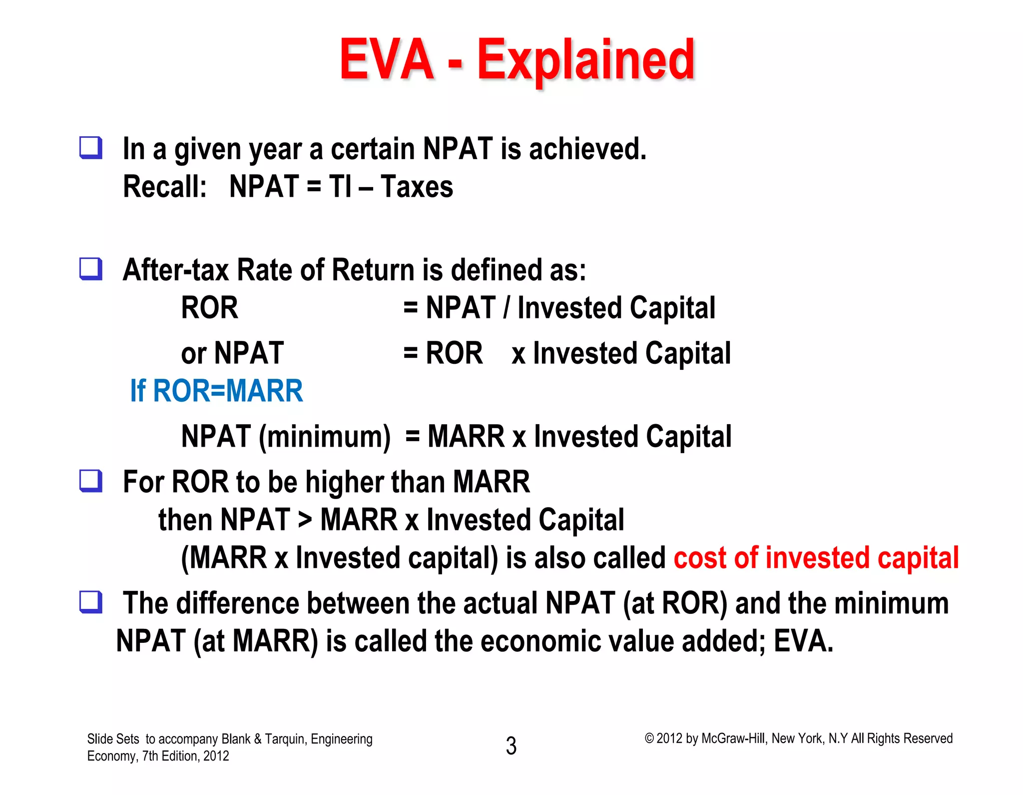
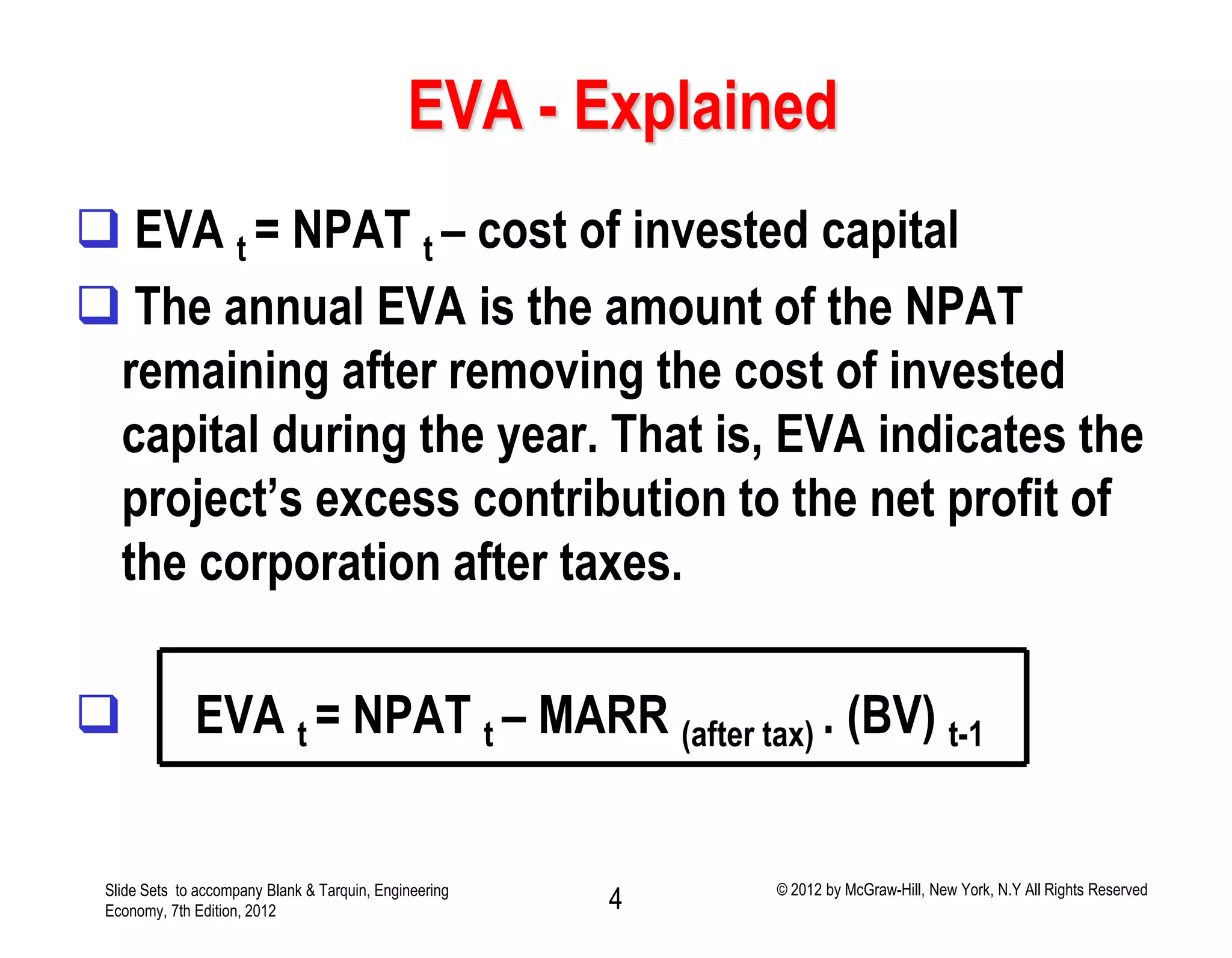
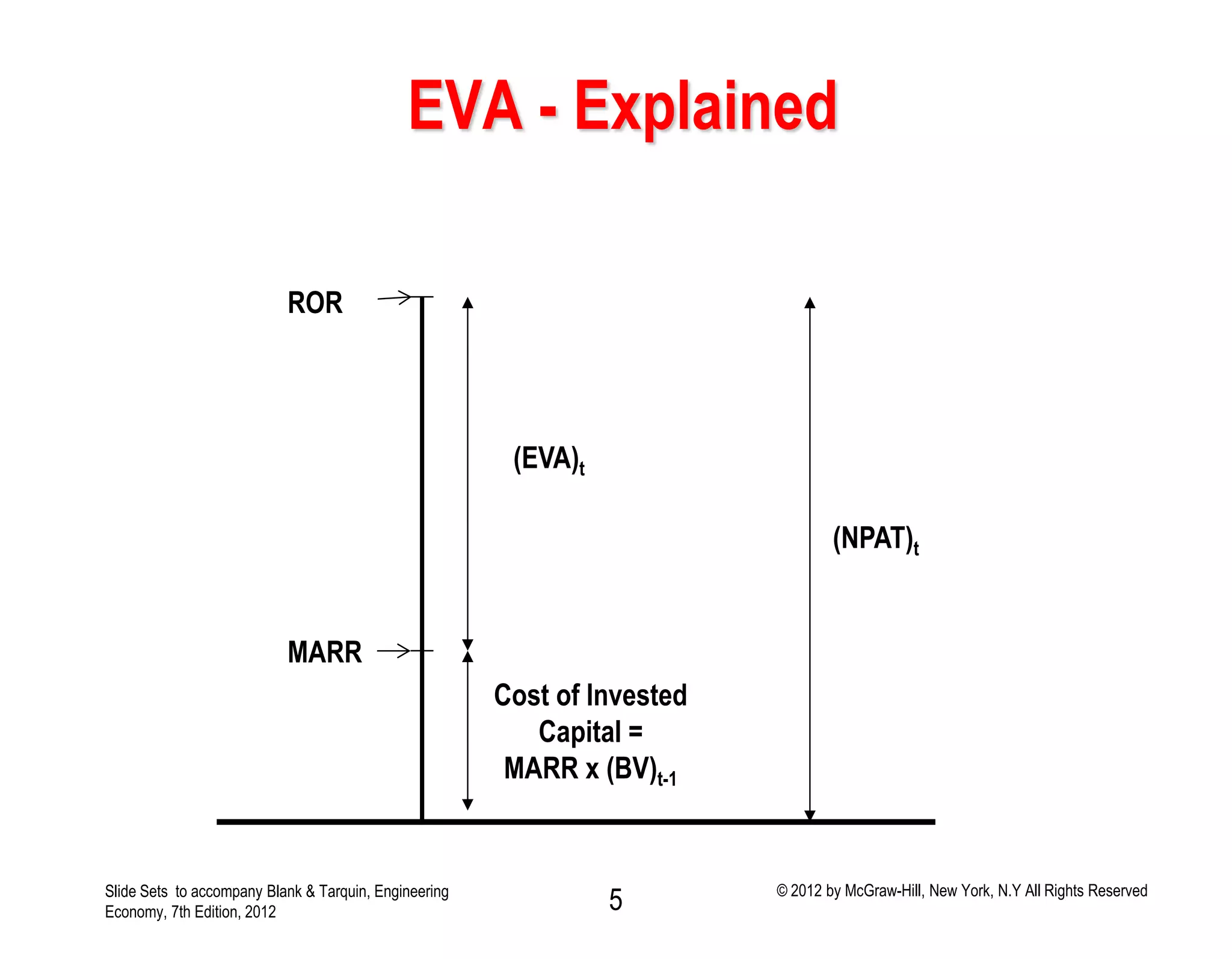
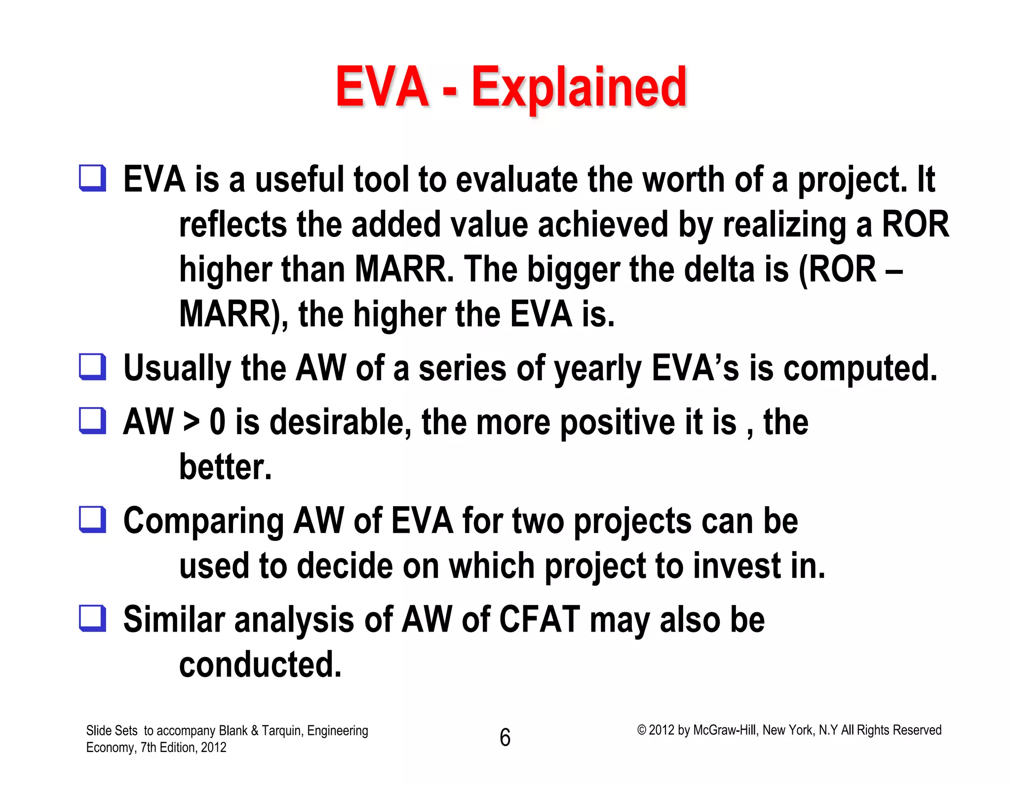
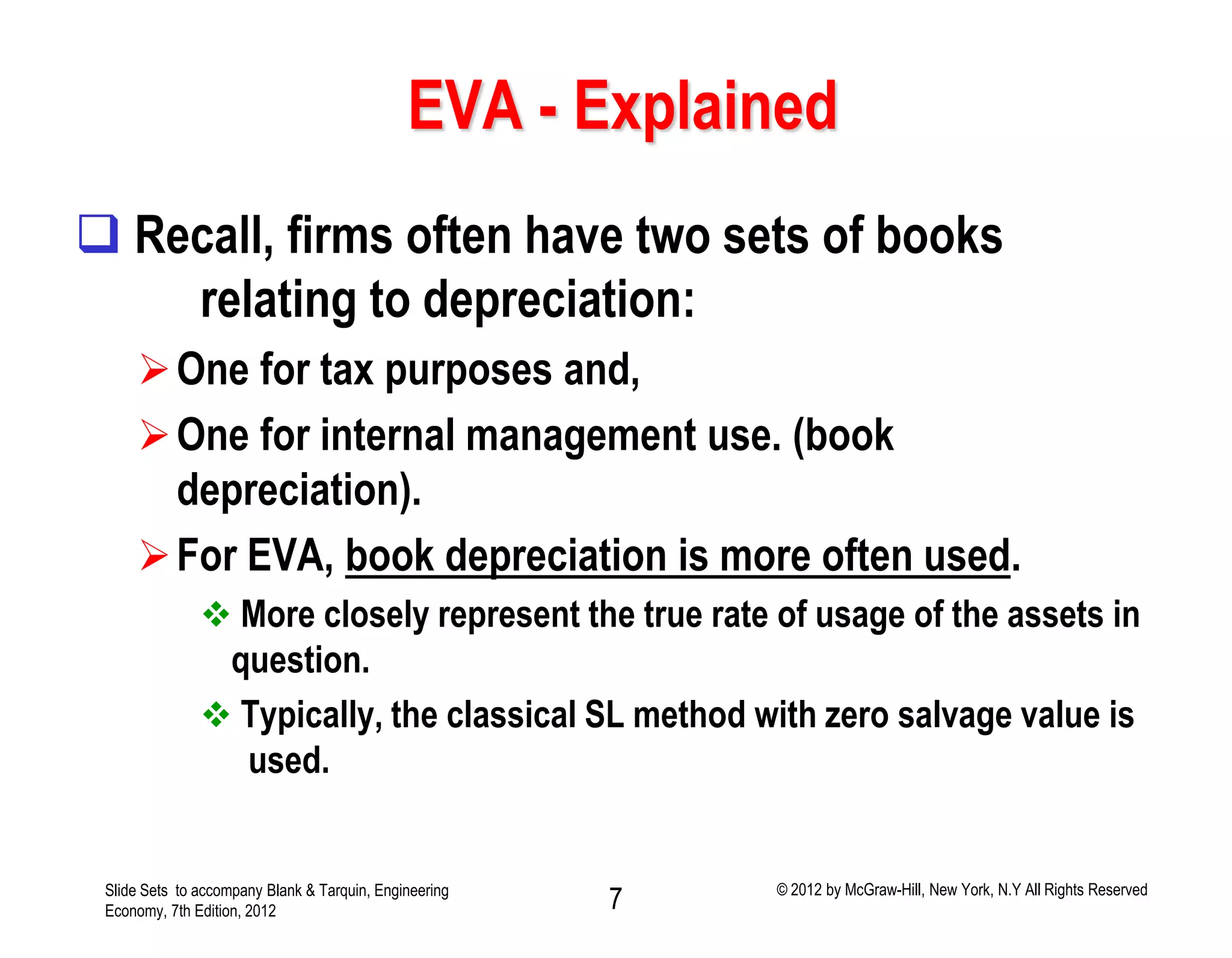


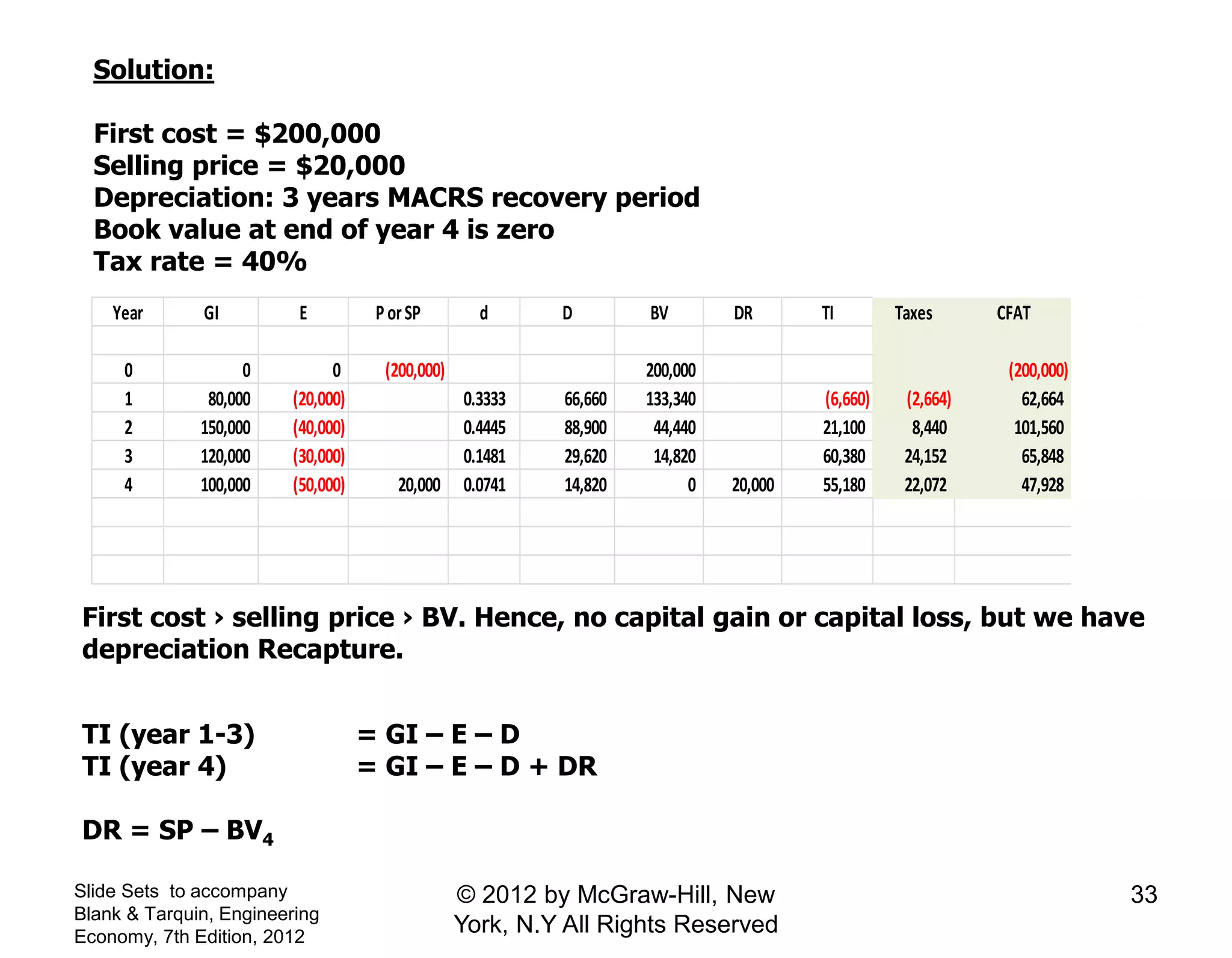
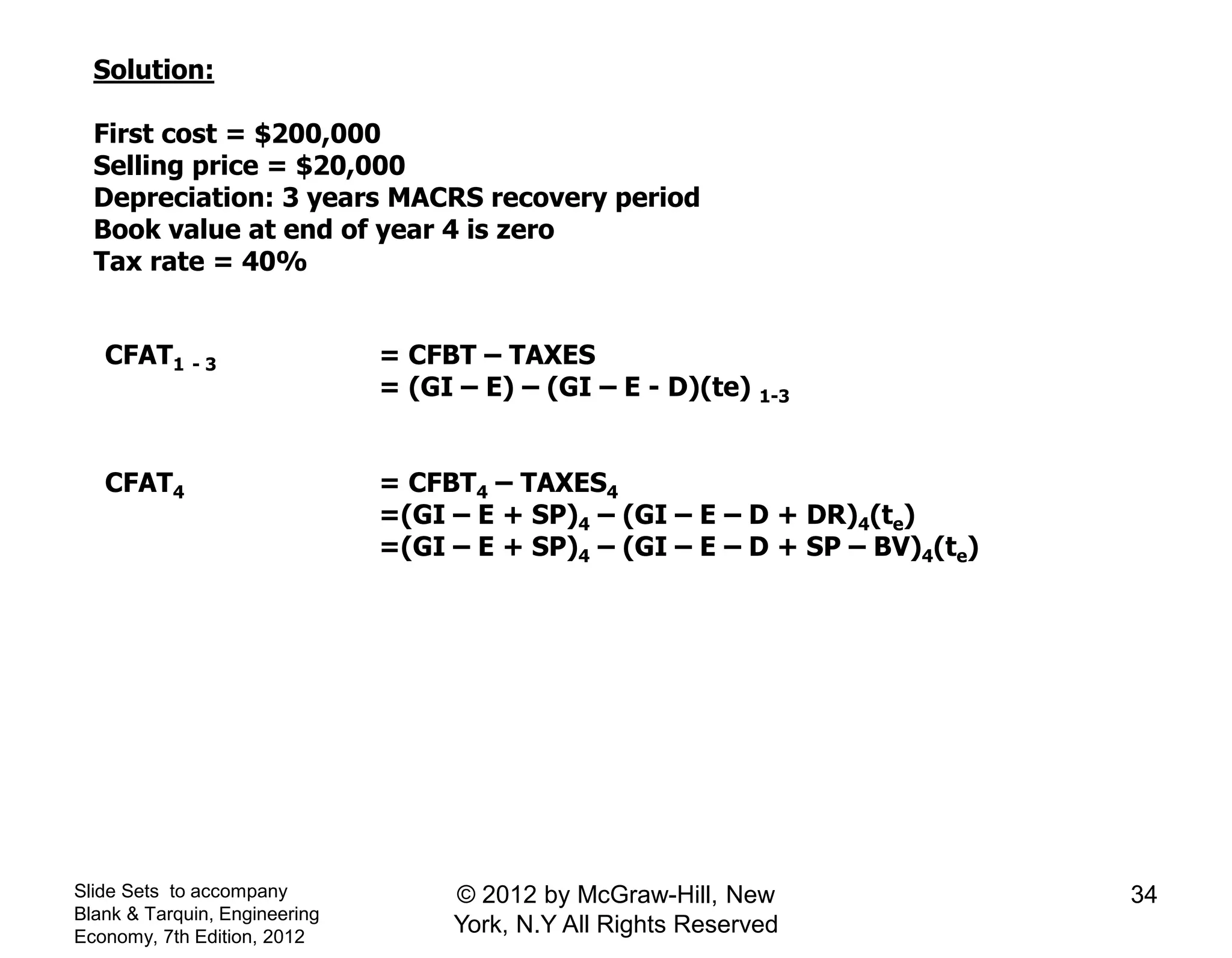

1) The document discusses economic value added (EVA) and how it is calculated as net profit after tax minus the cost of invested capital. 2) EVA indicates the excess contribution to net profit after removing the minimum required return. It is useful for evaluating investment projects. 3) The document provides an example calculation of EVA and cash flow analysis for a project over 4 years to demonstrate how the analyses are economically equivalent. Both show the project is not justified at the 12% after-tax hurdle rate.


