This chapter discusses uncertainty and rational responses to it. It introduces key concepts like states of nature, contingent contracts and consumption plans, and state-contingent budget constraints. Rational agents will choose the most preferred affordable consumption plan from their budget set. Insurance is a common response to reduce the costs of uncertainty. Competitive insurance leads to "fair" prices where risk-averse agents buy full insurance. Diversification and mutual insurance are other ways to manage risk.

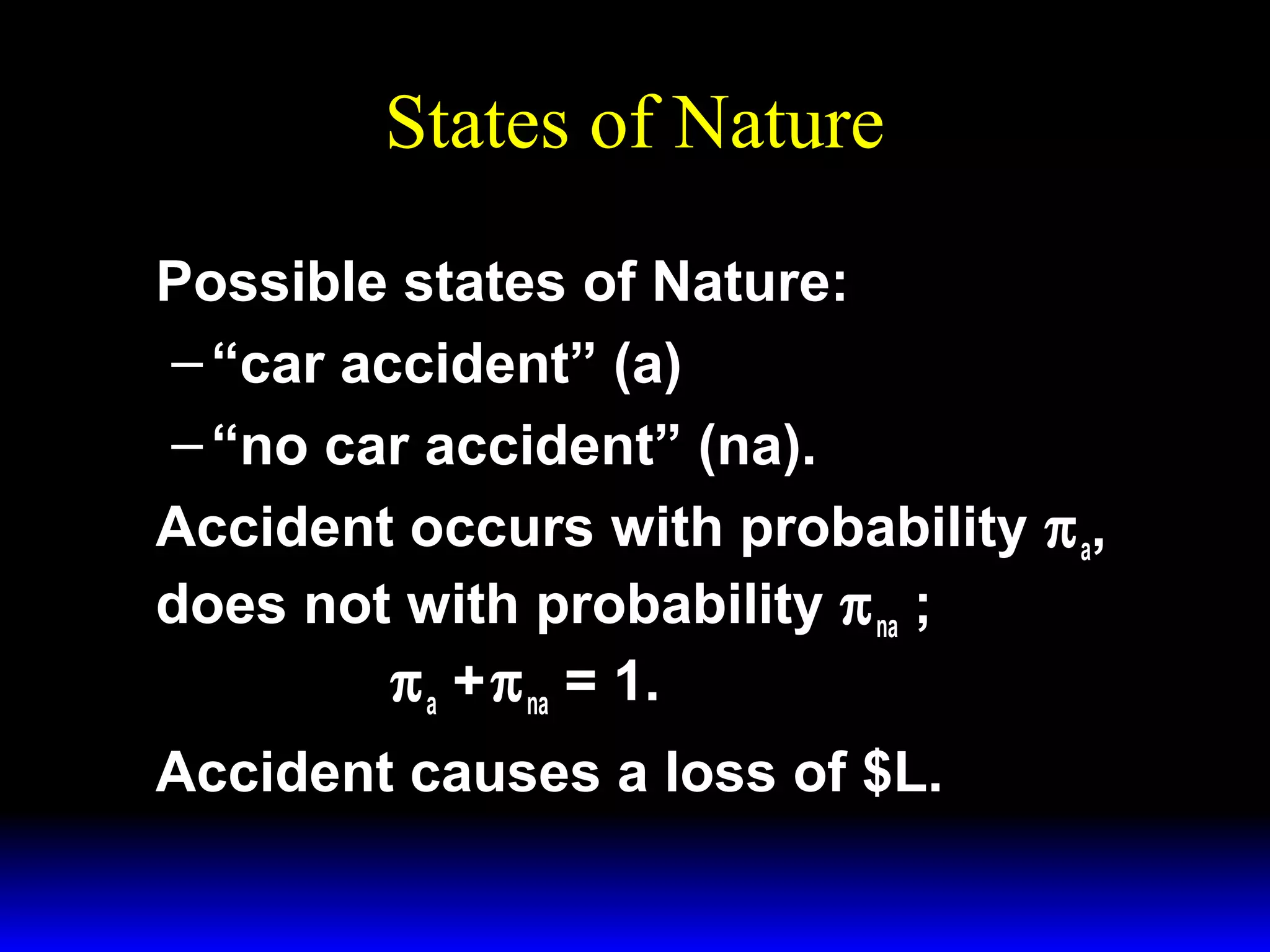
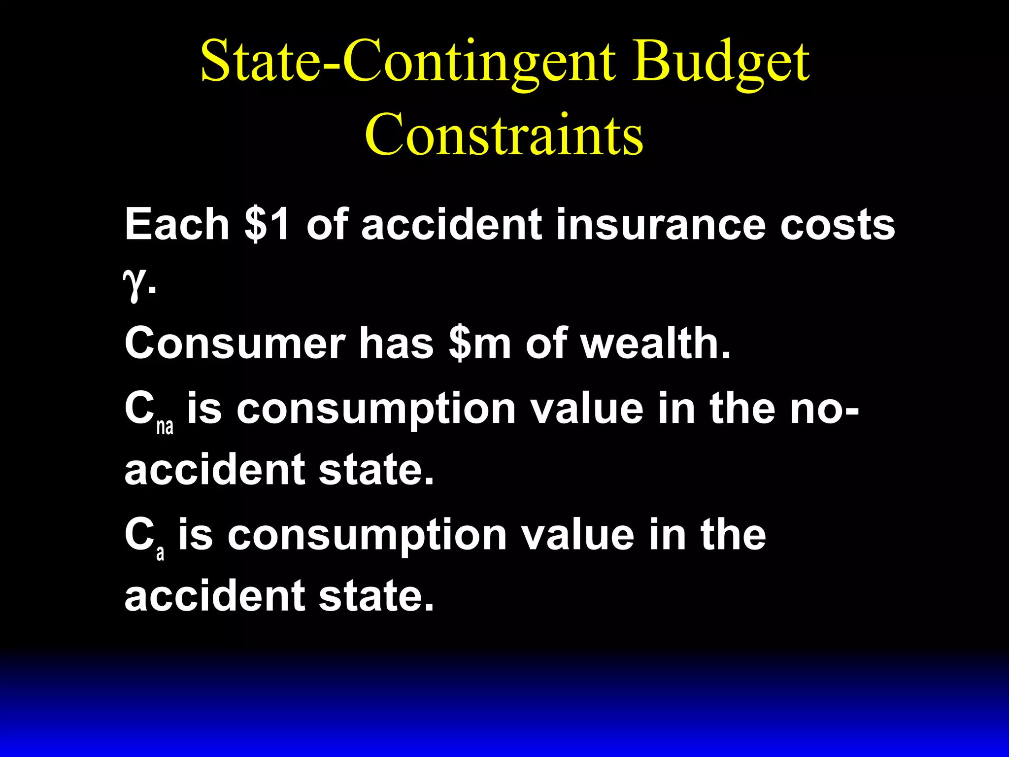
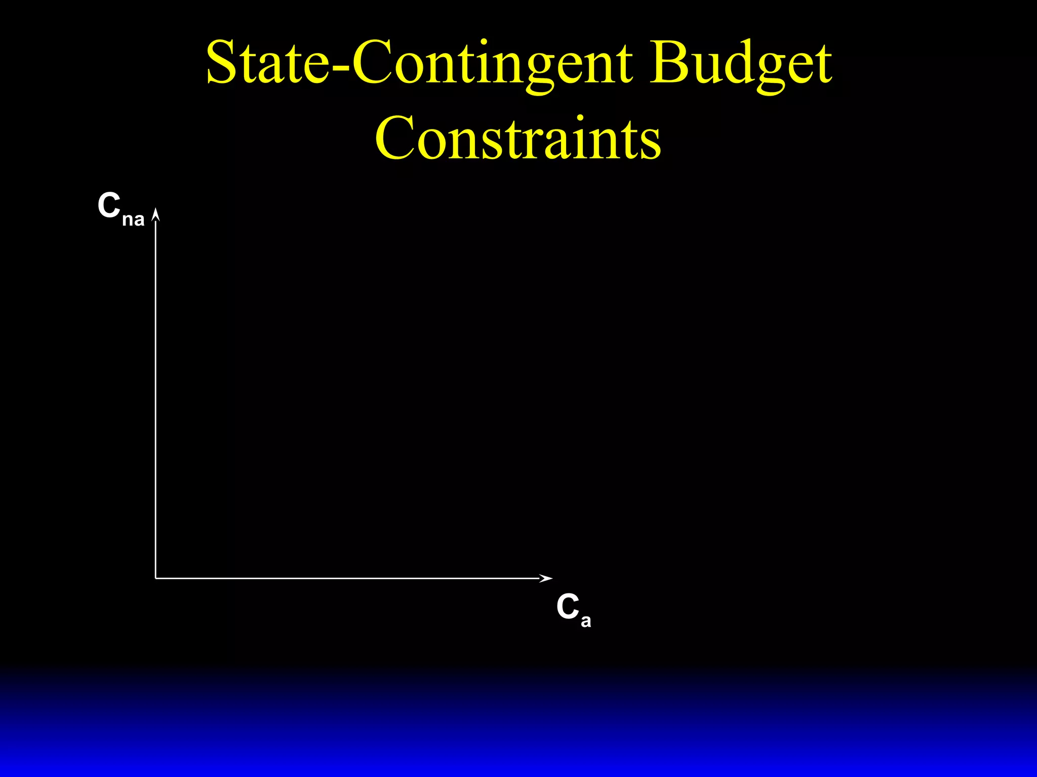
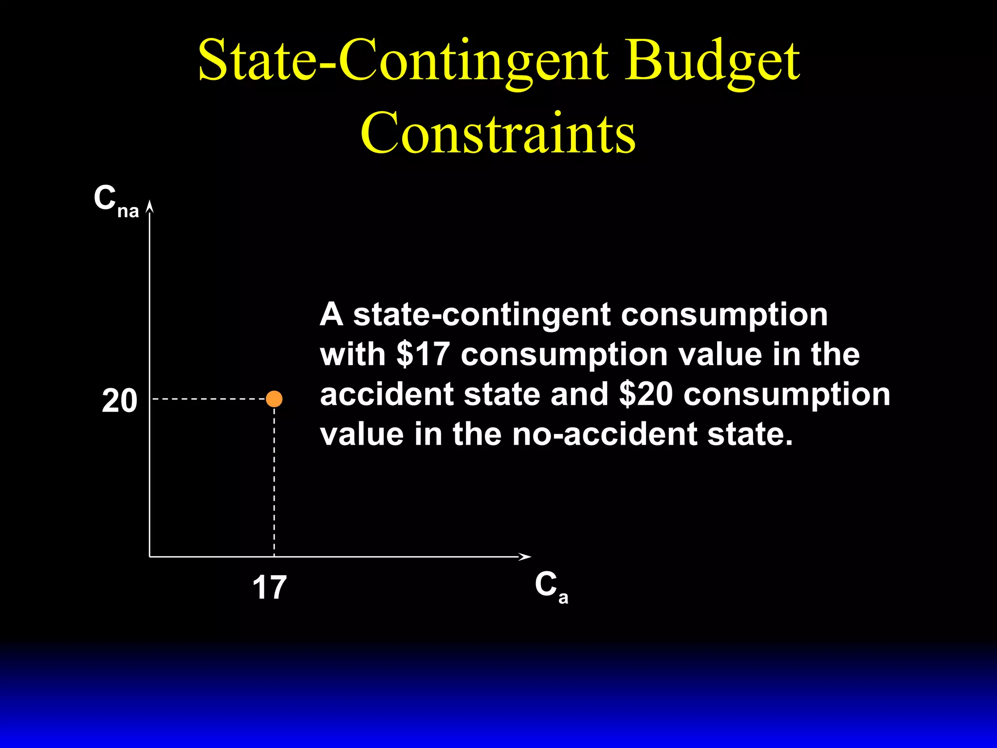
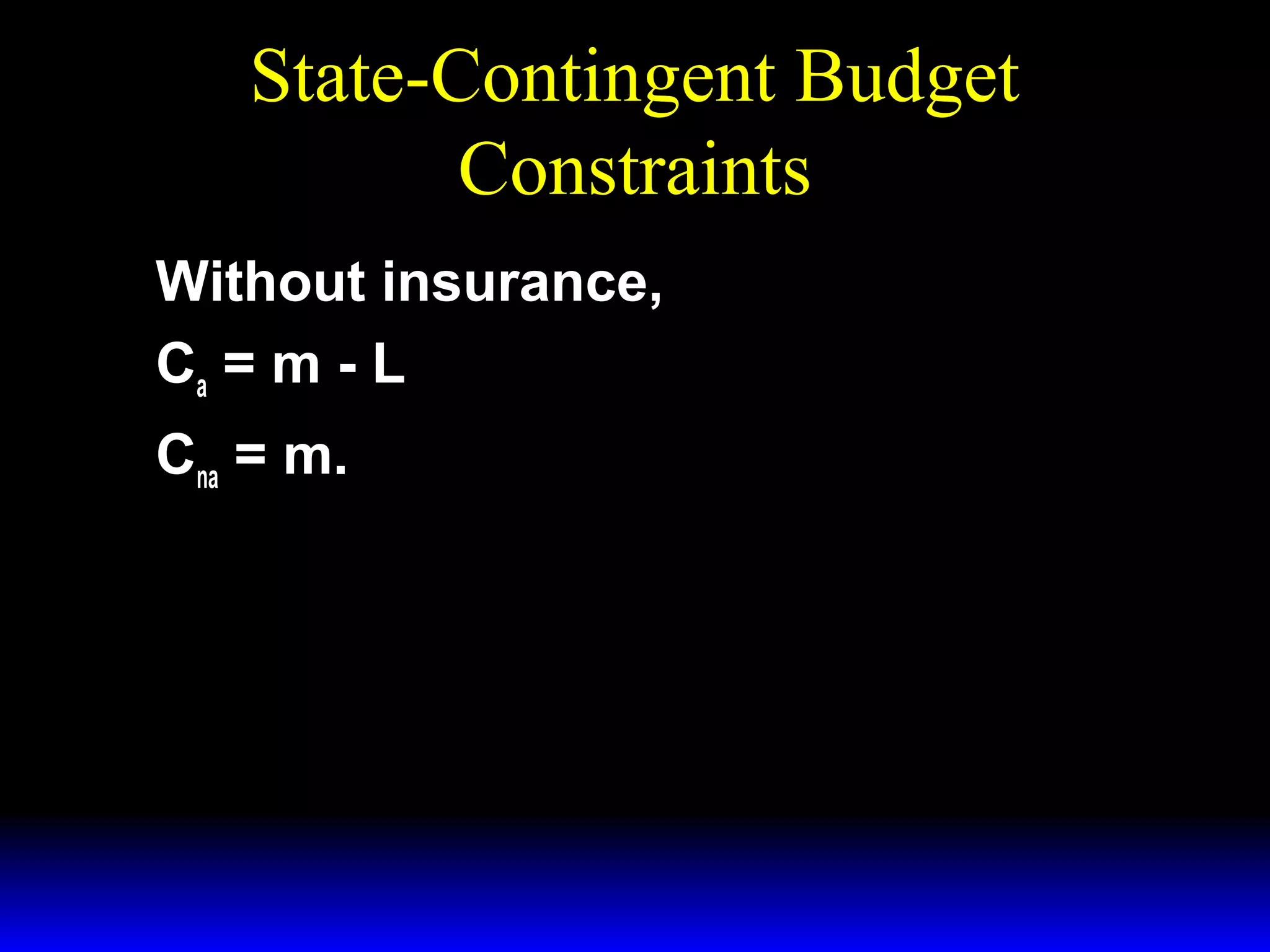
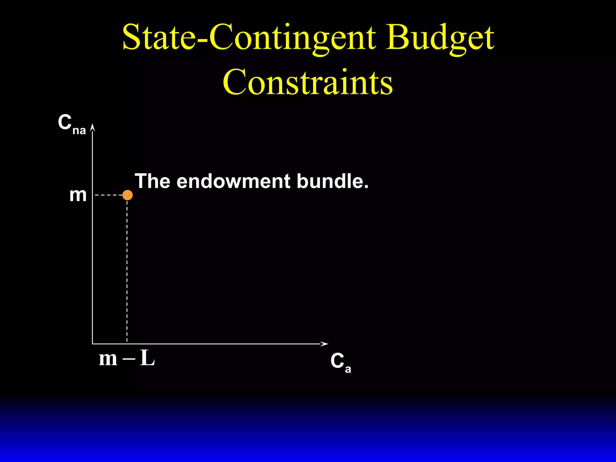
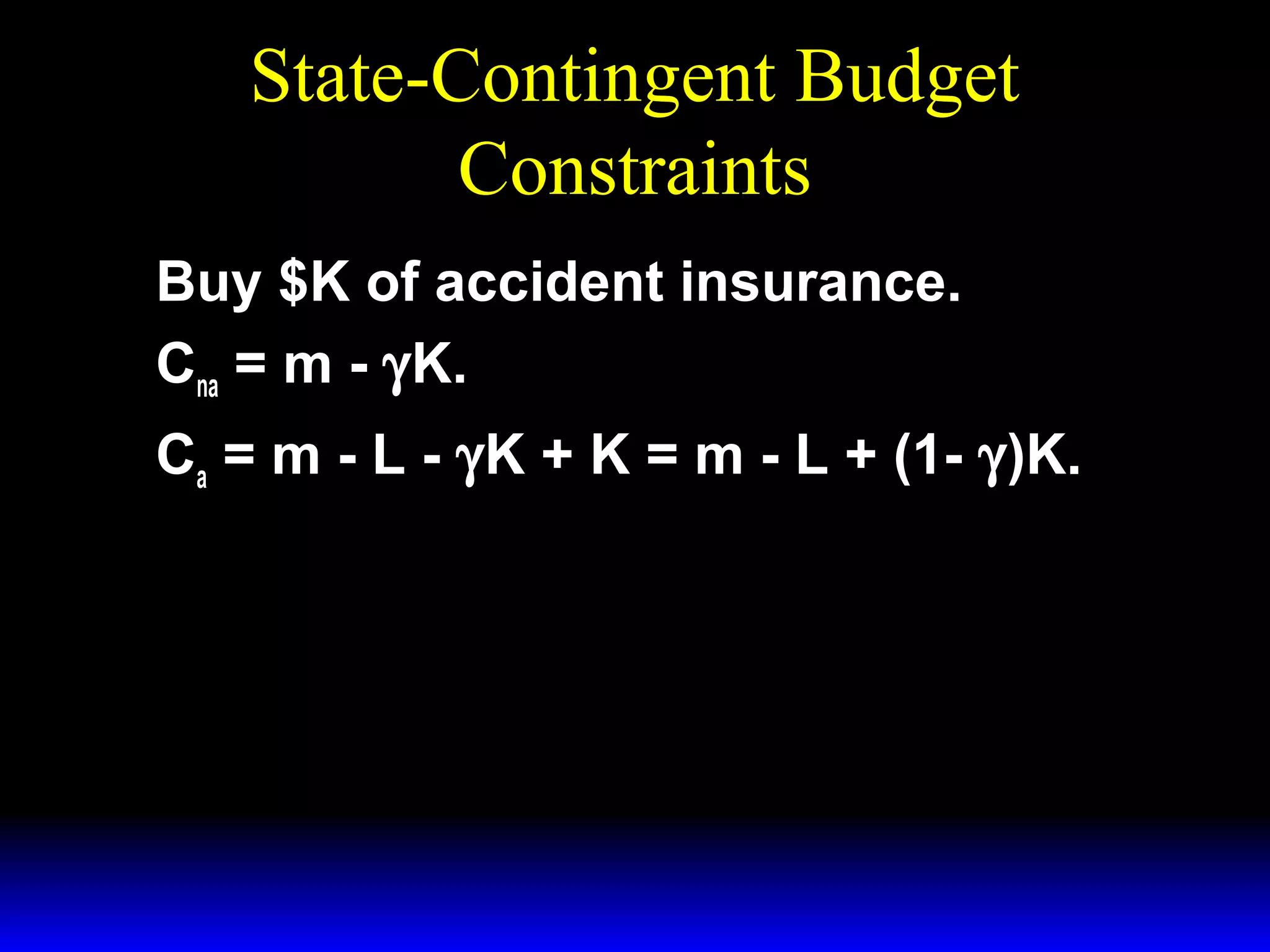
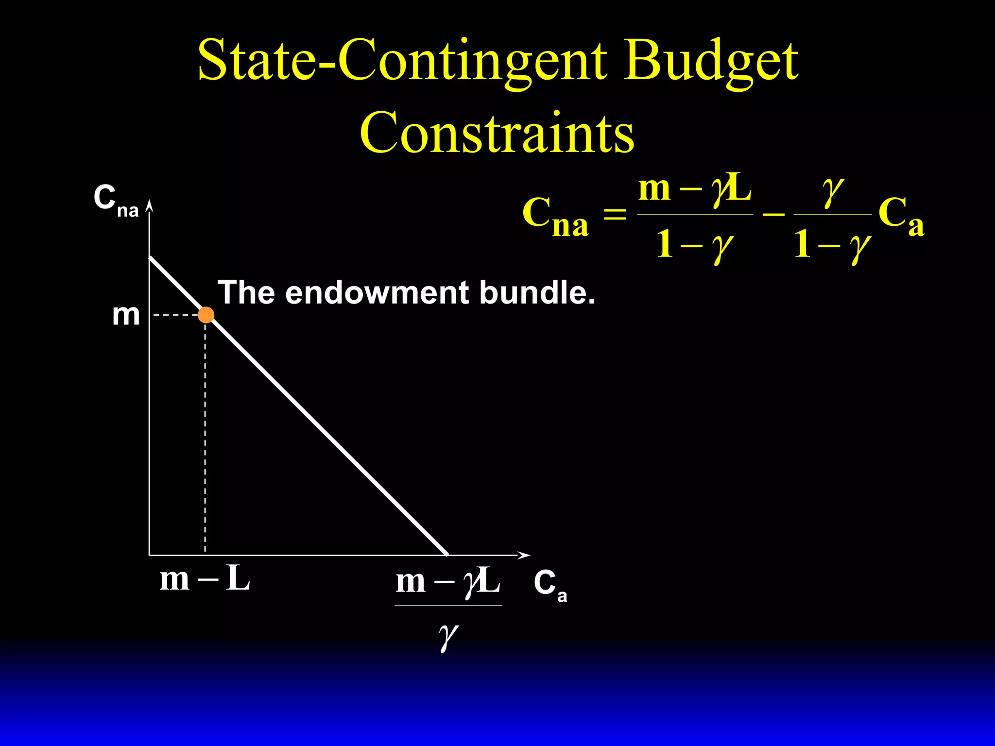
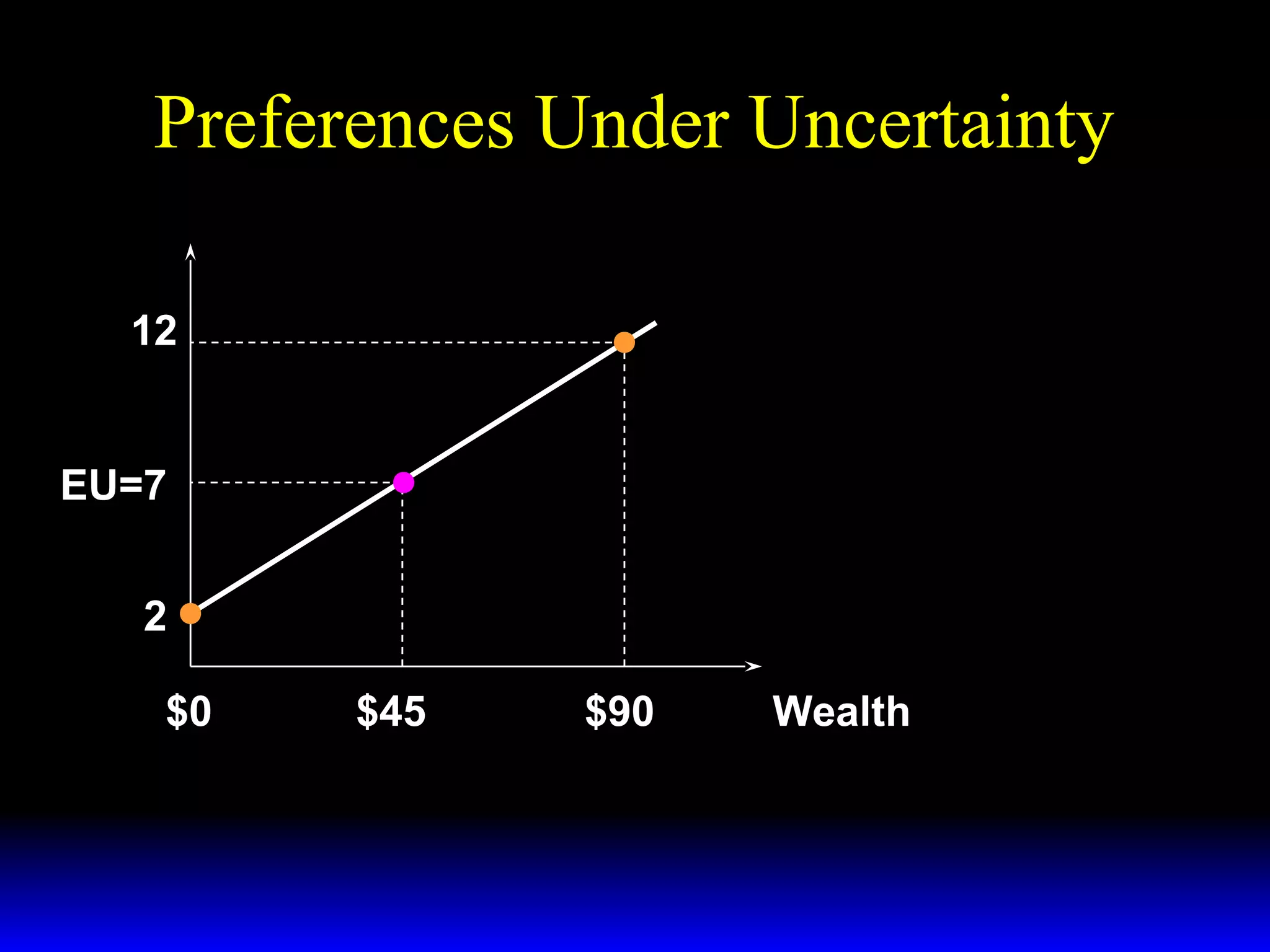
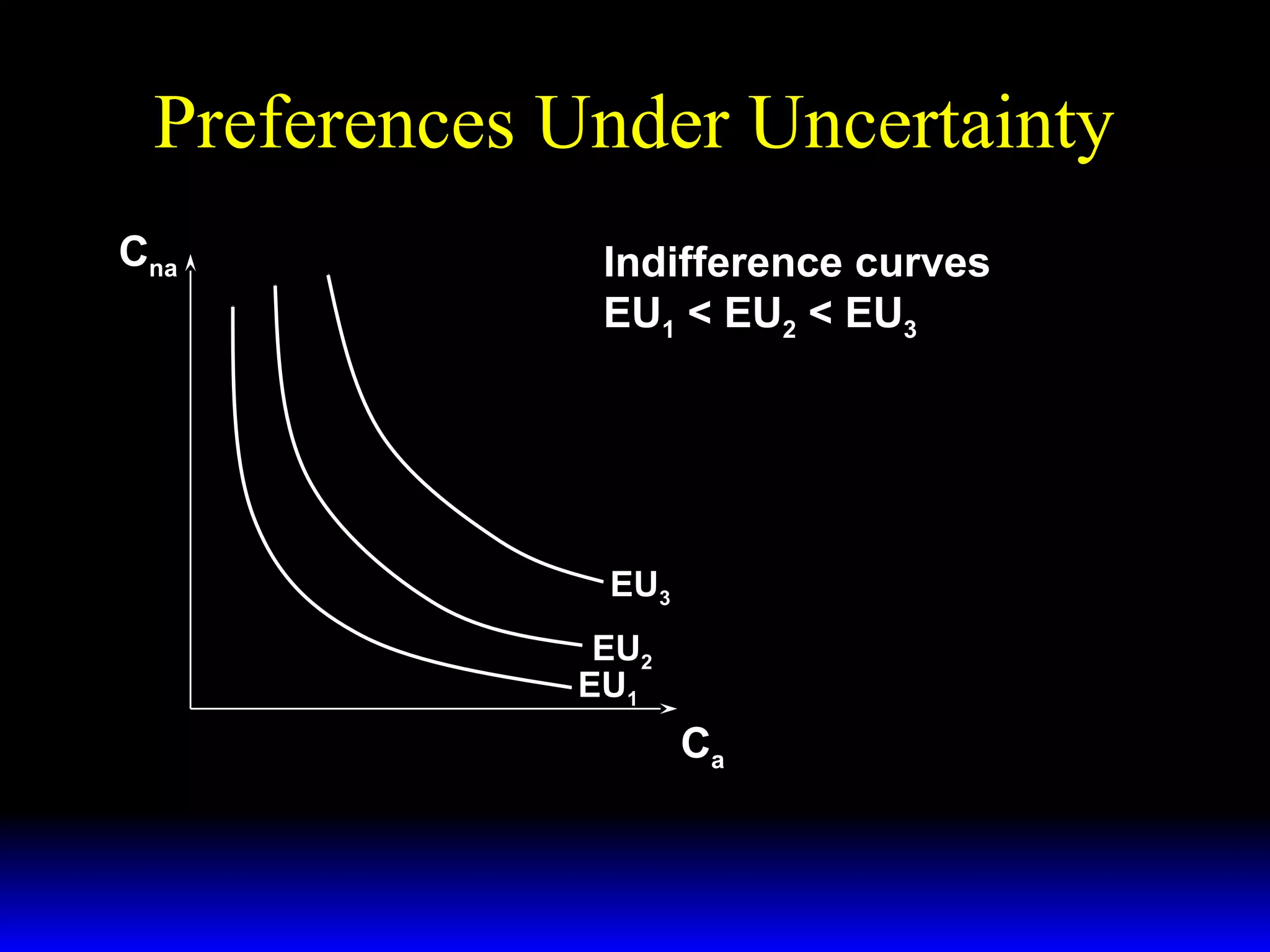
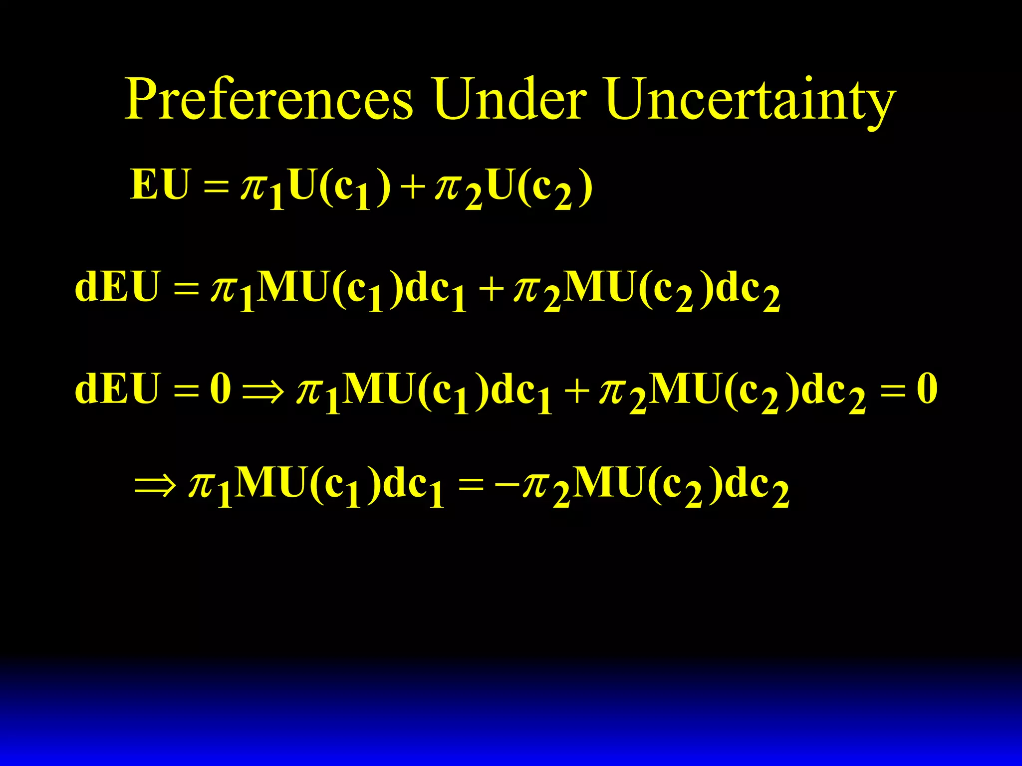
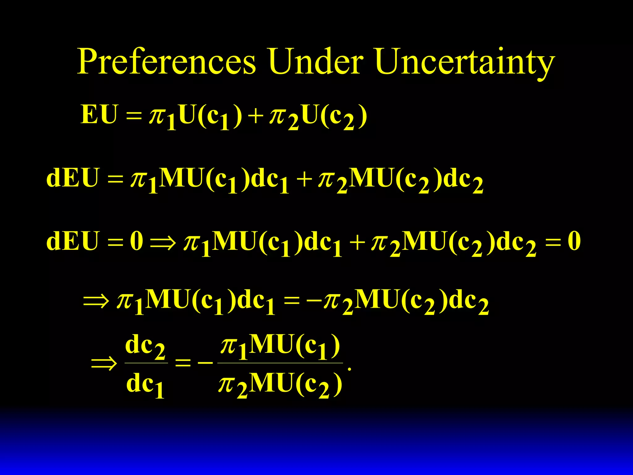
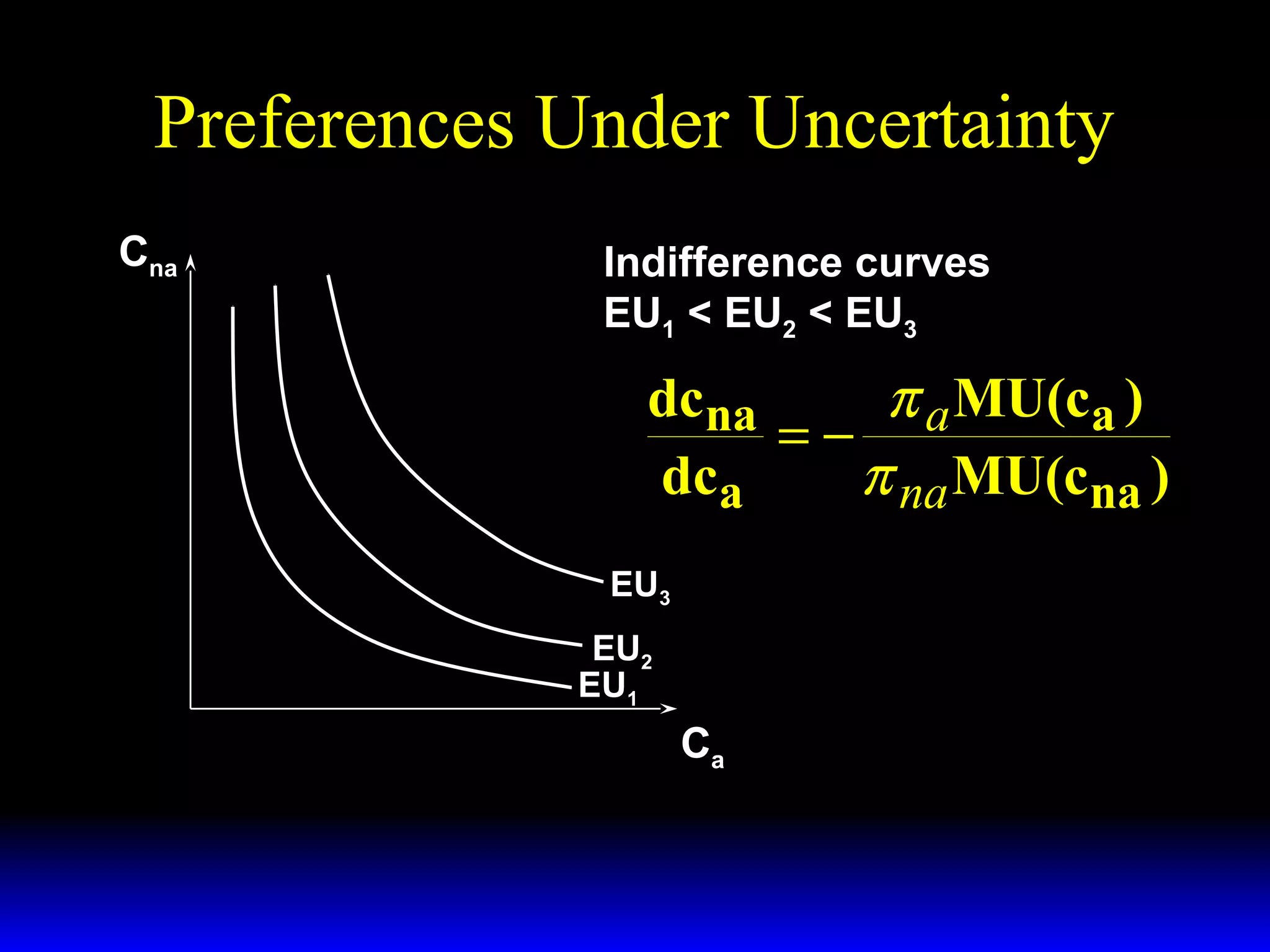
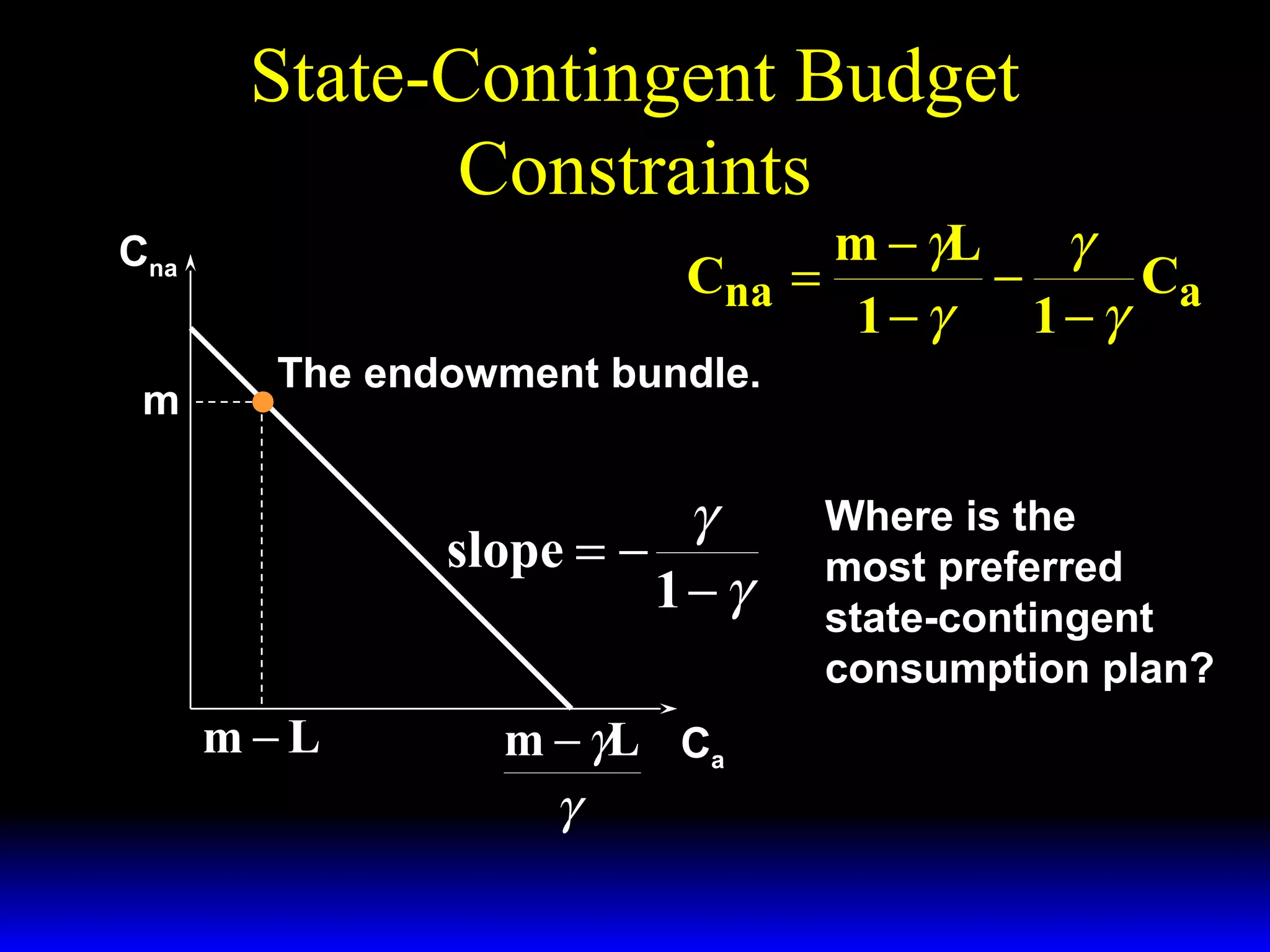
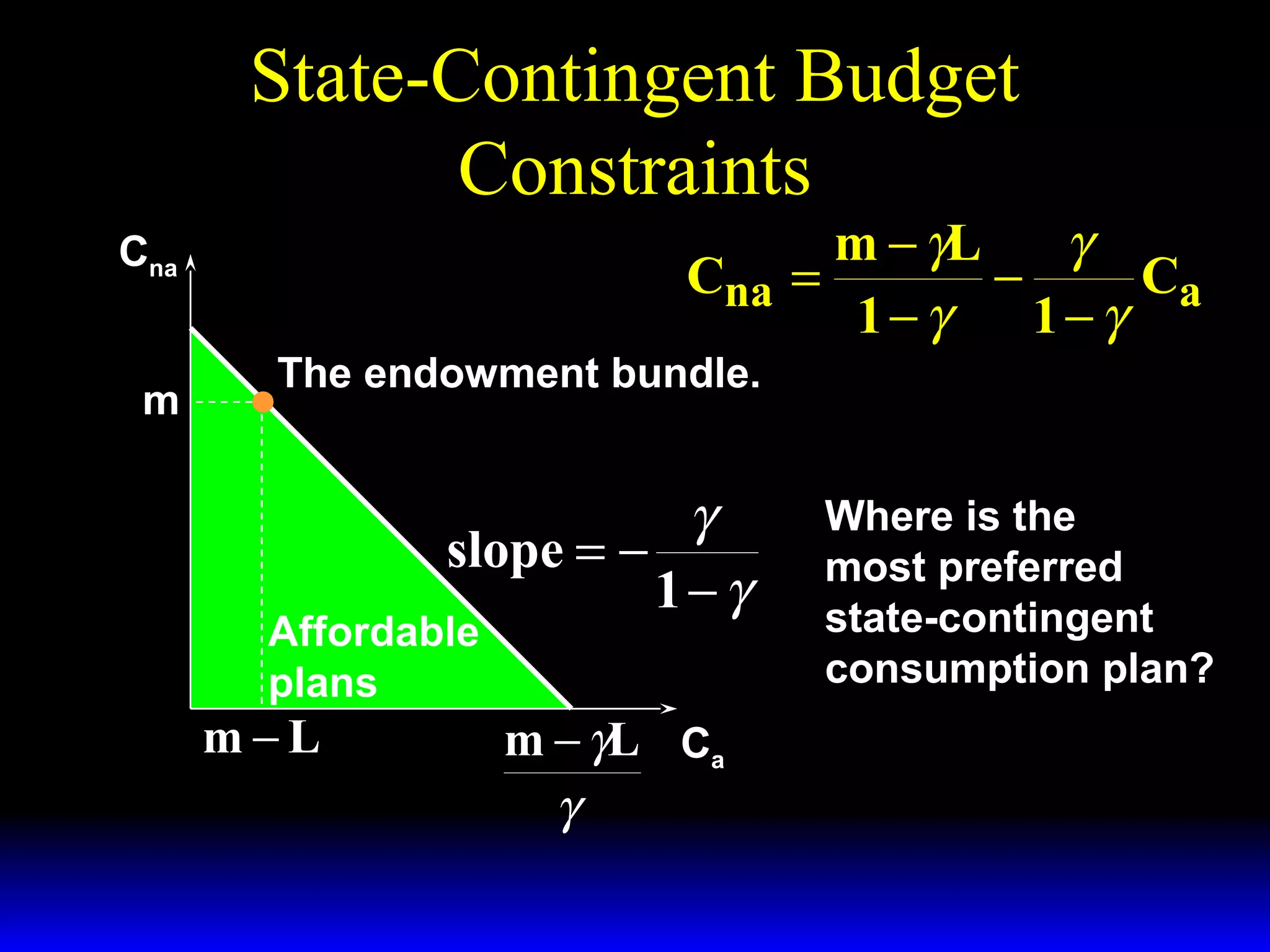
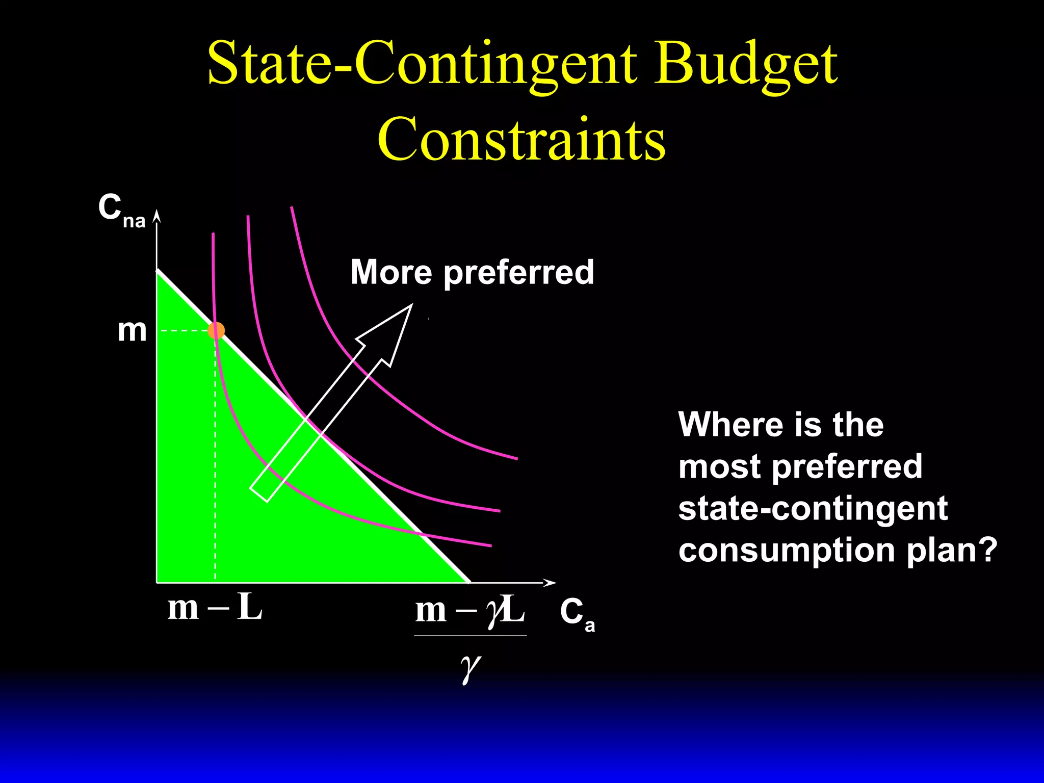
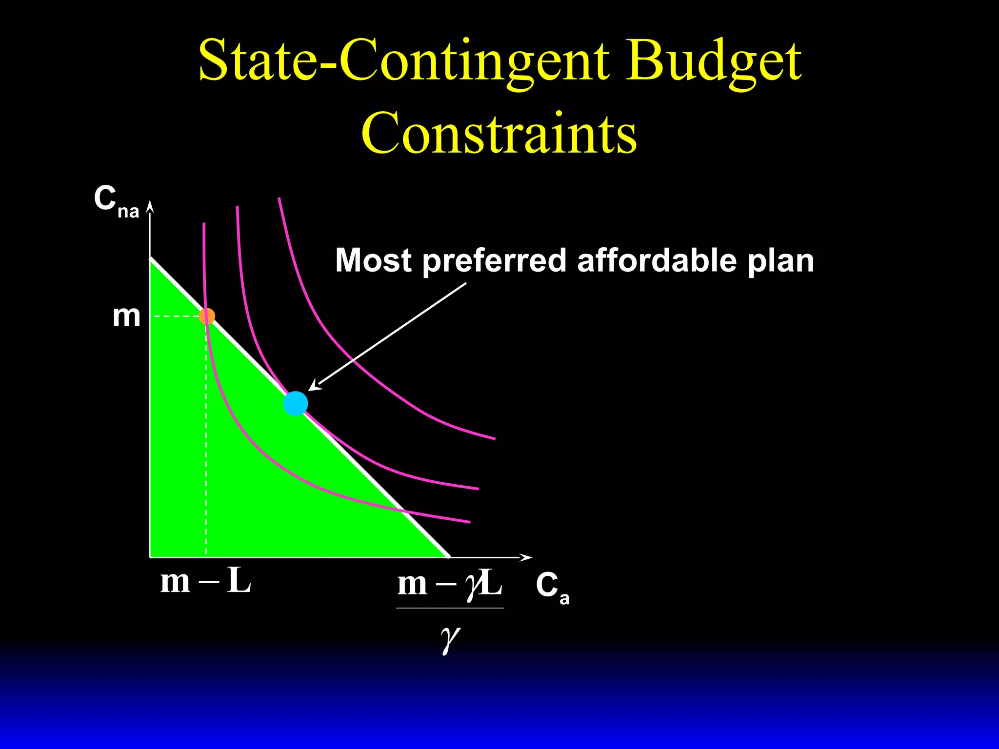
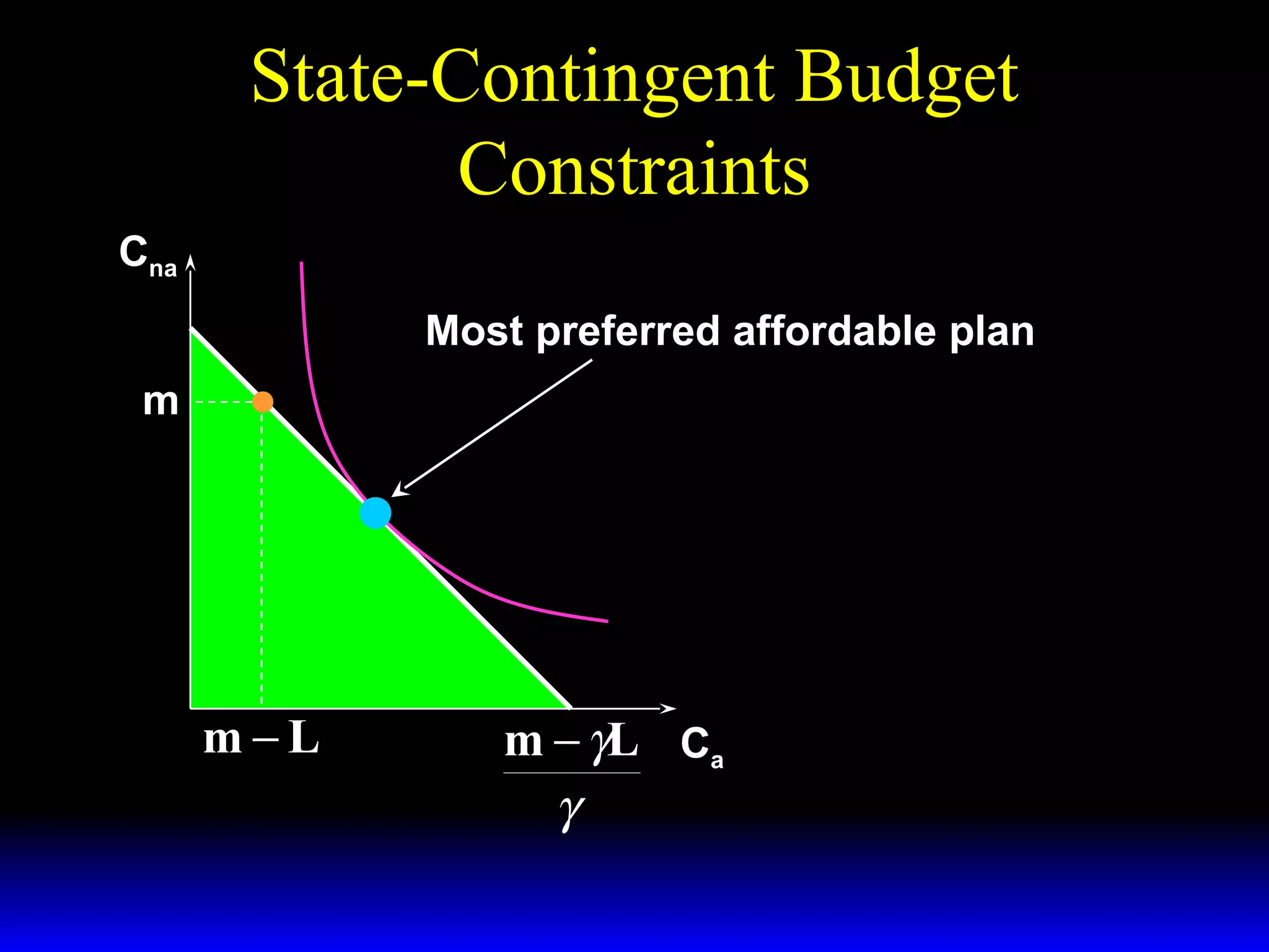
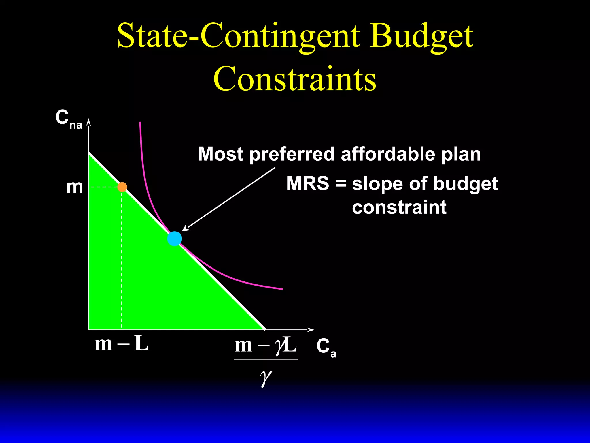
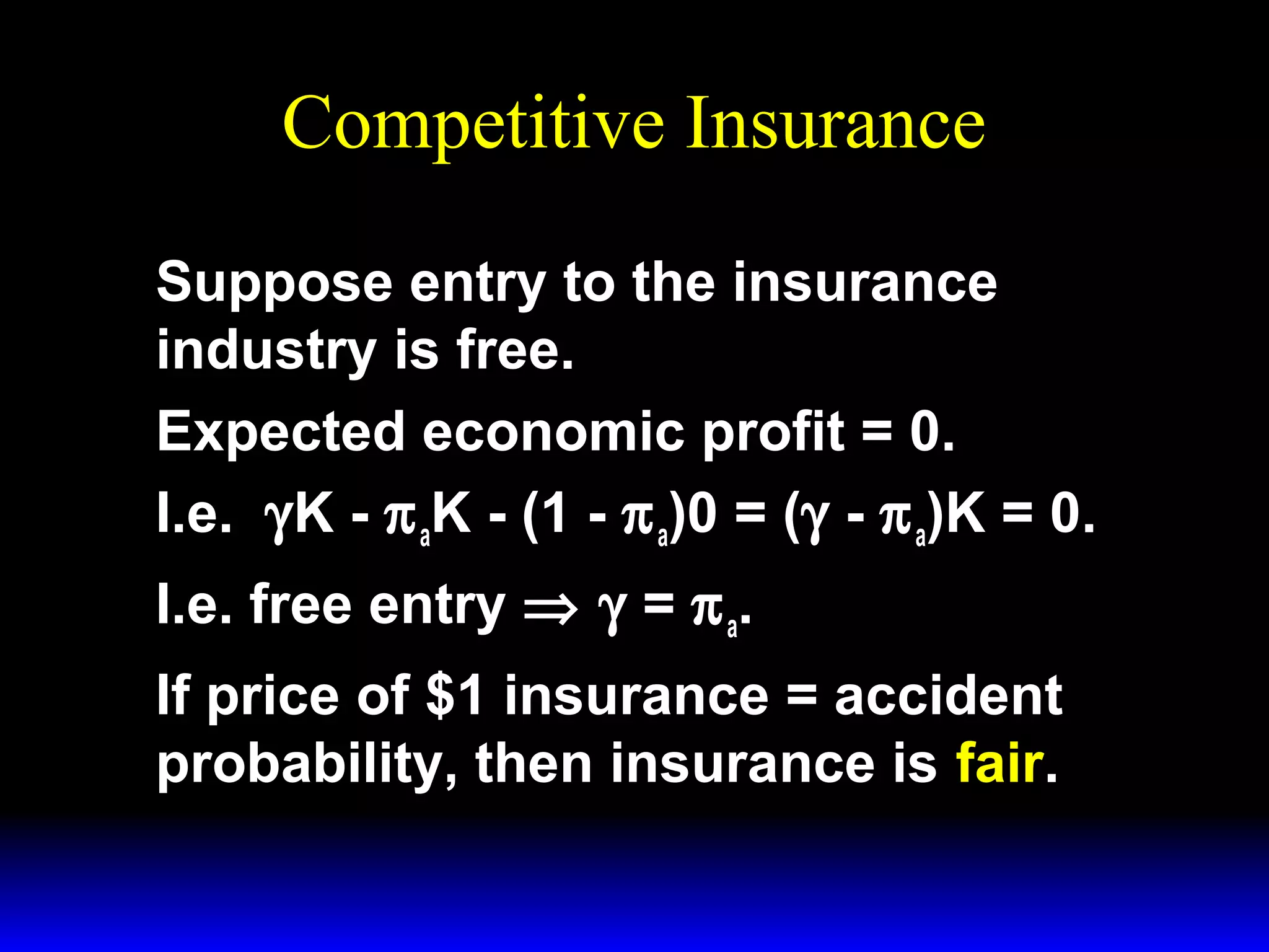
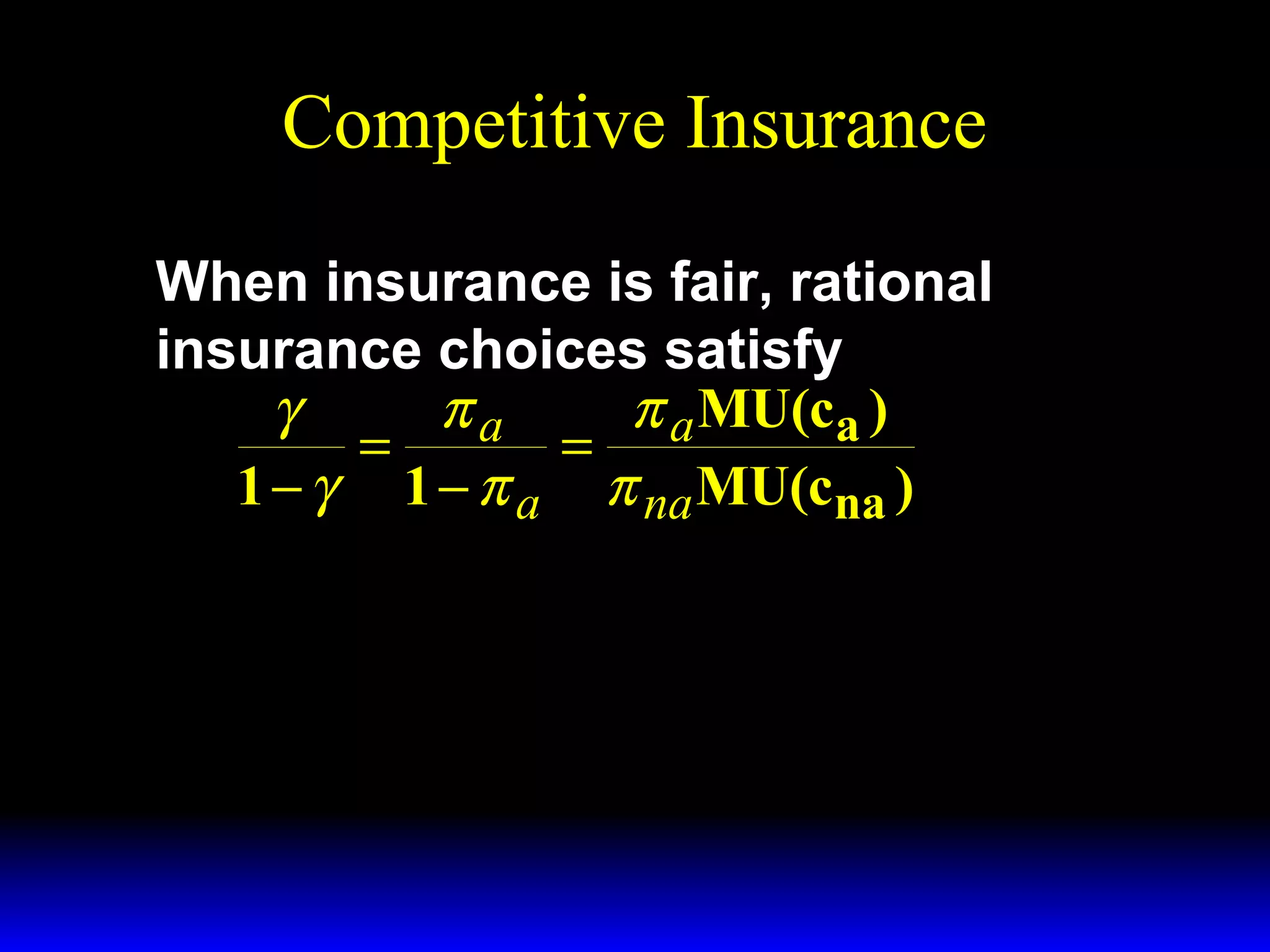
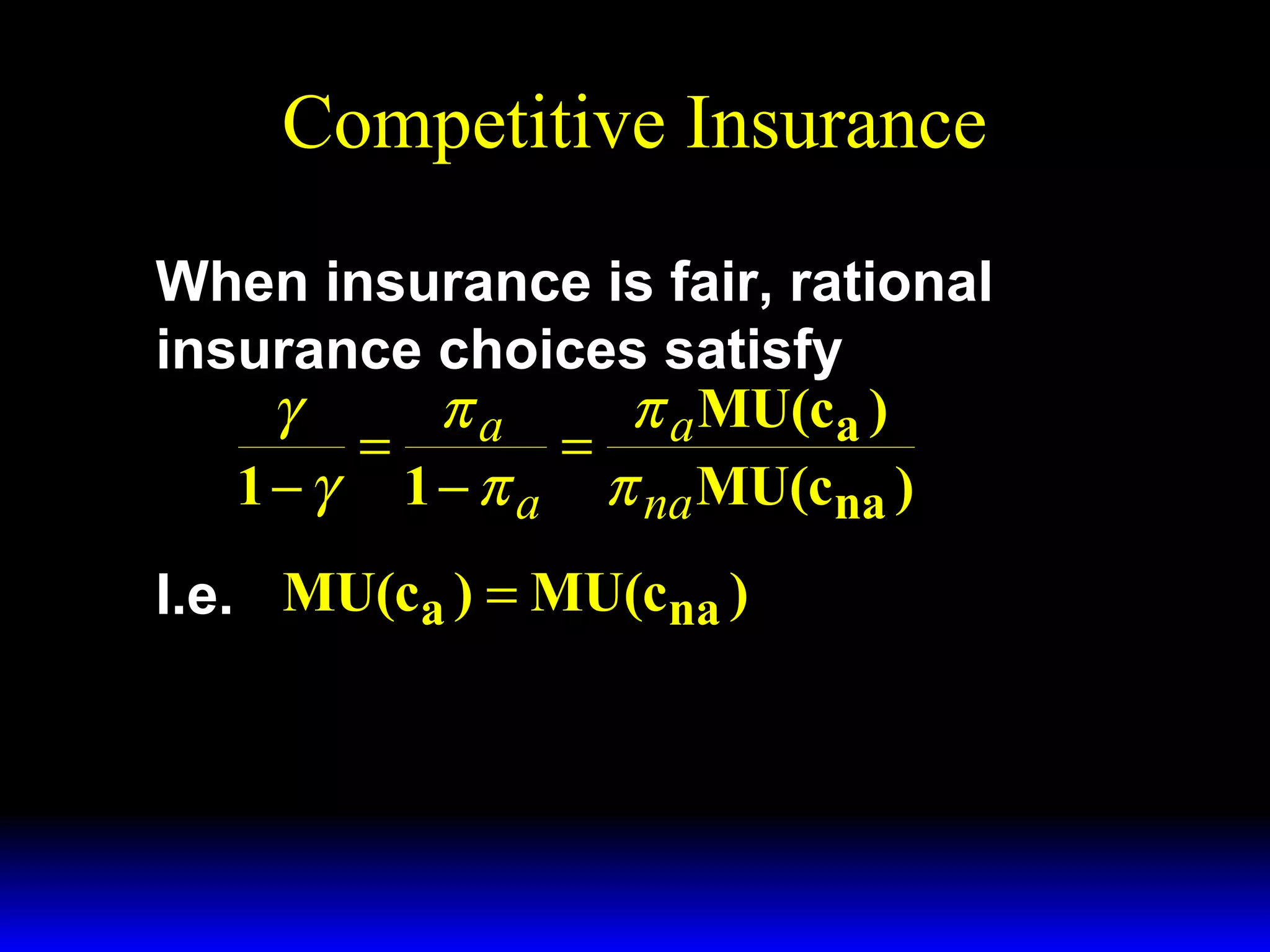
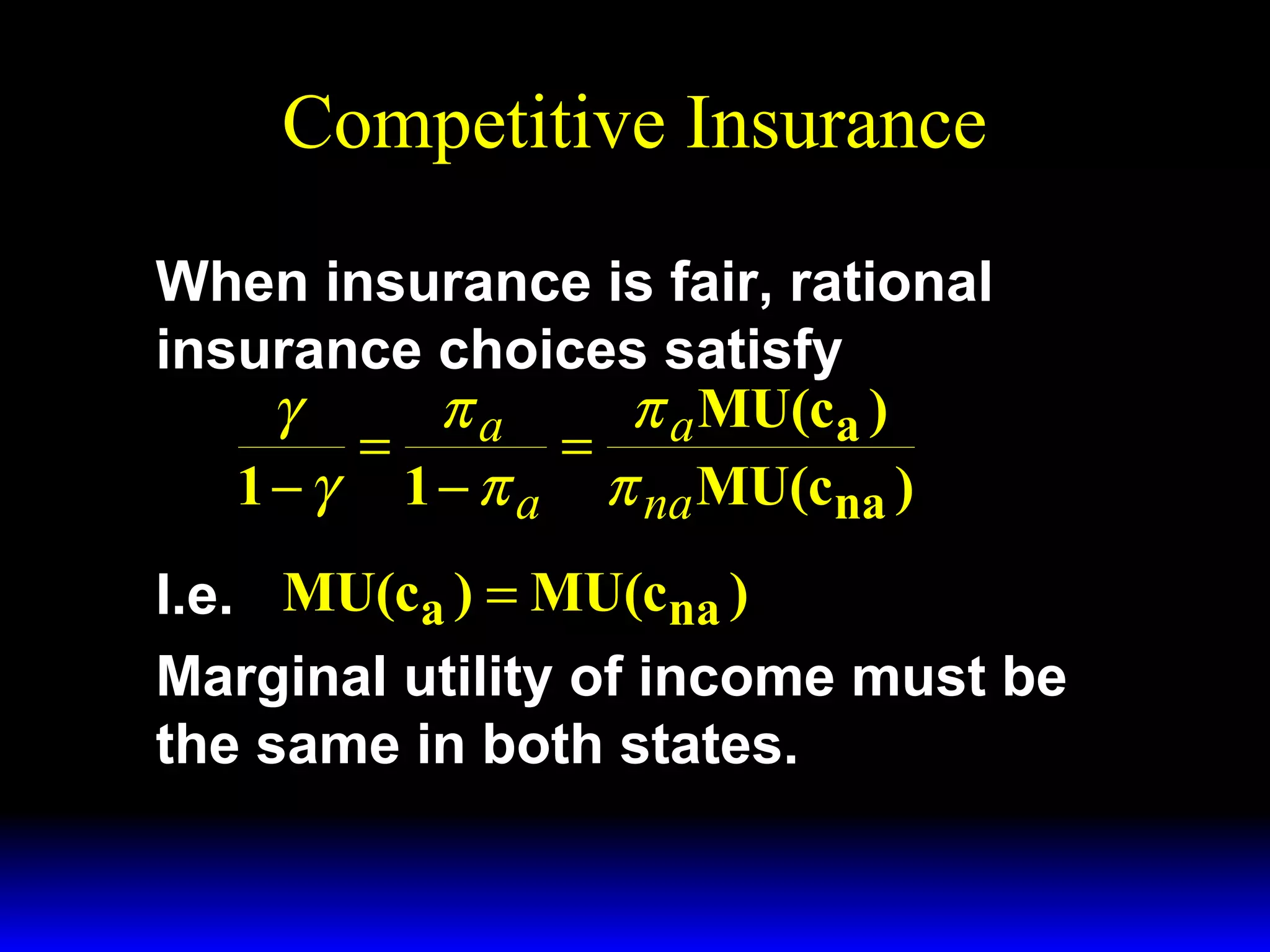
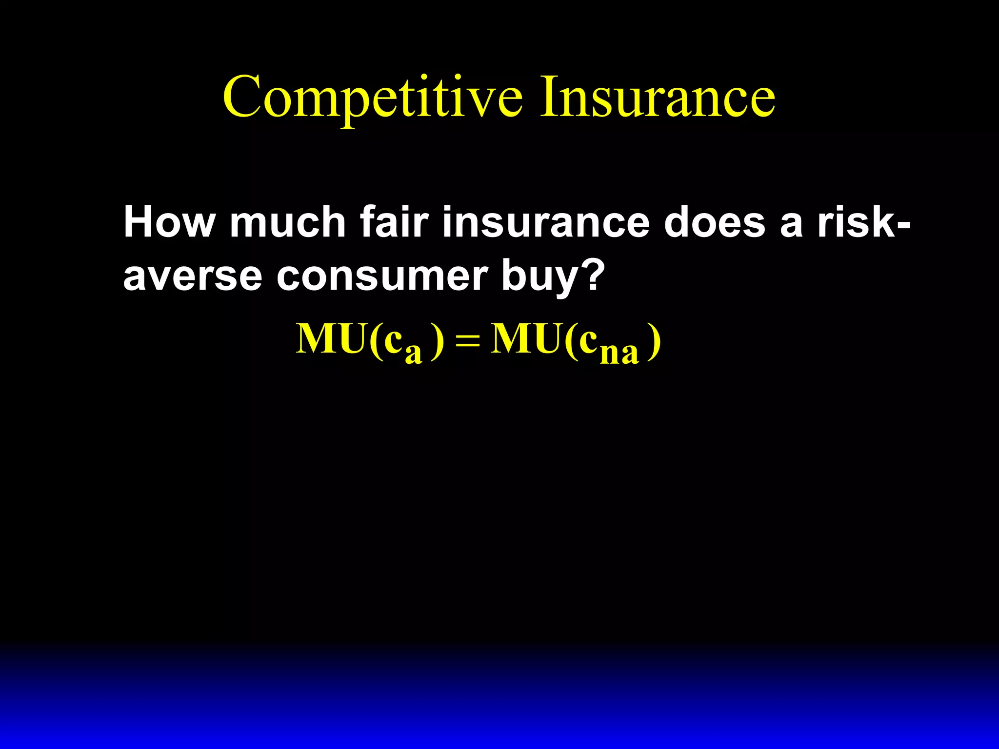
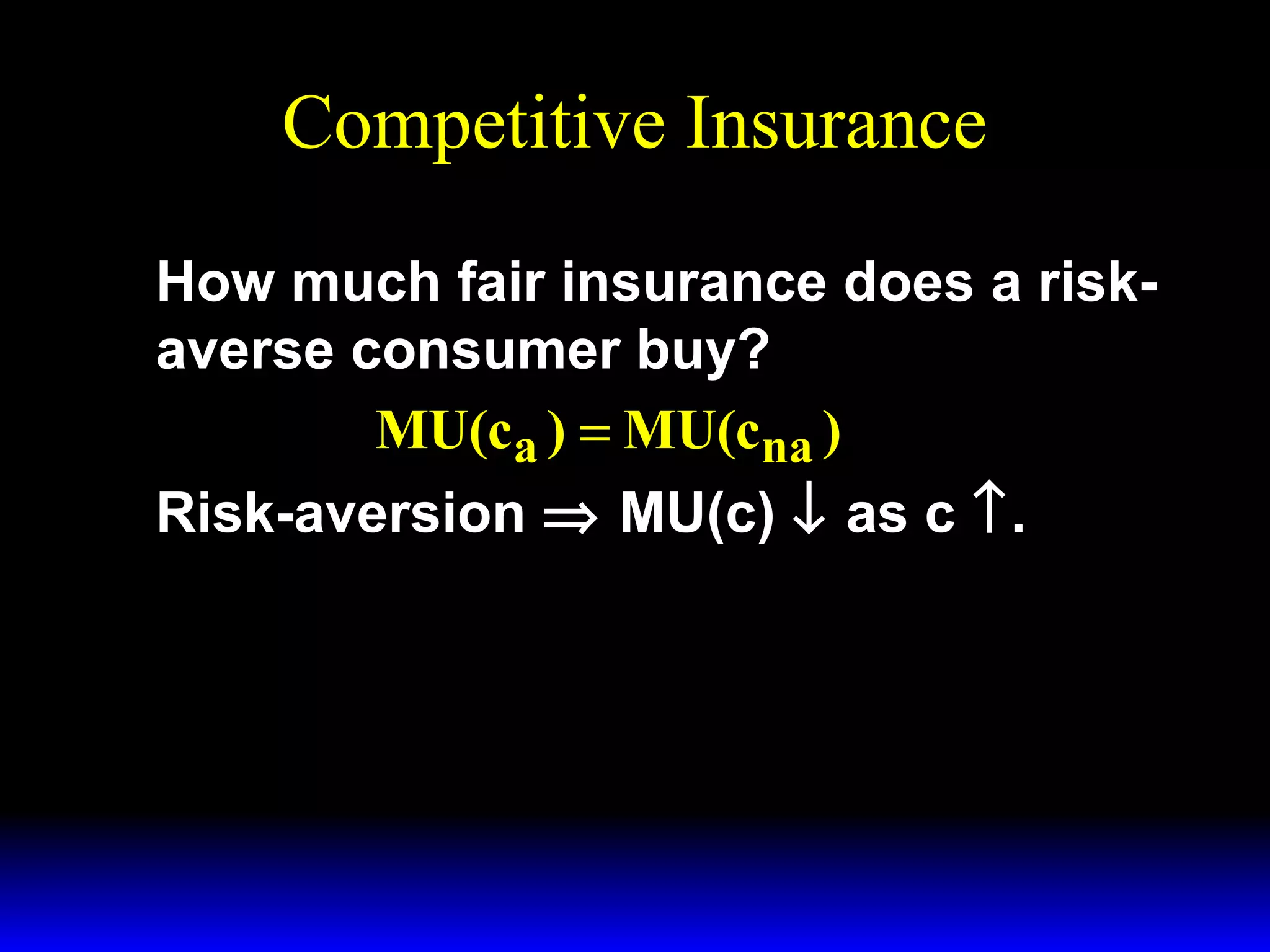
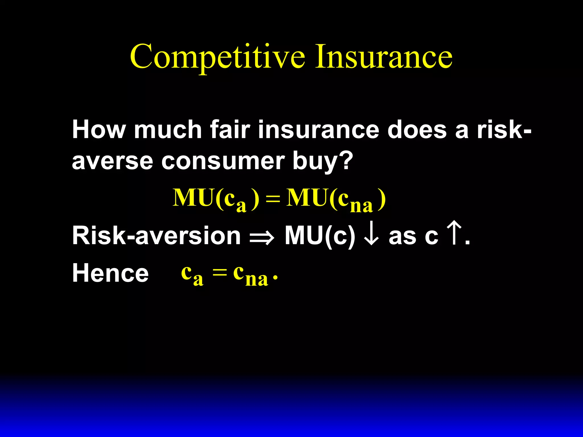
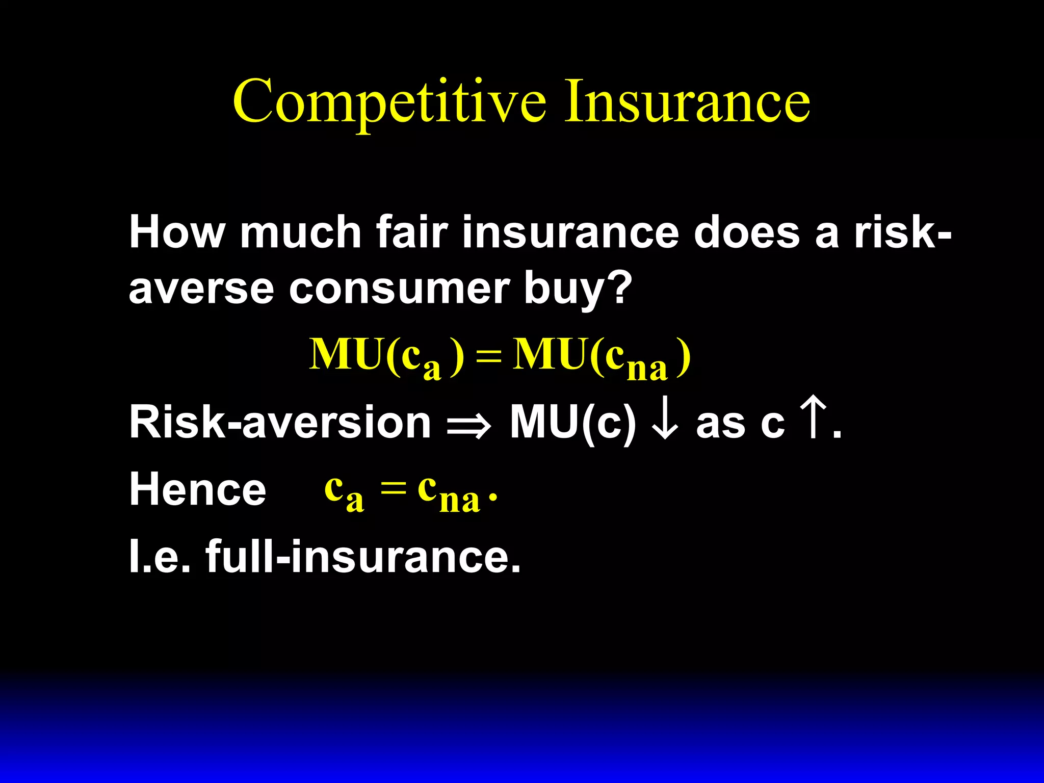
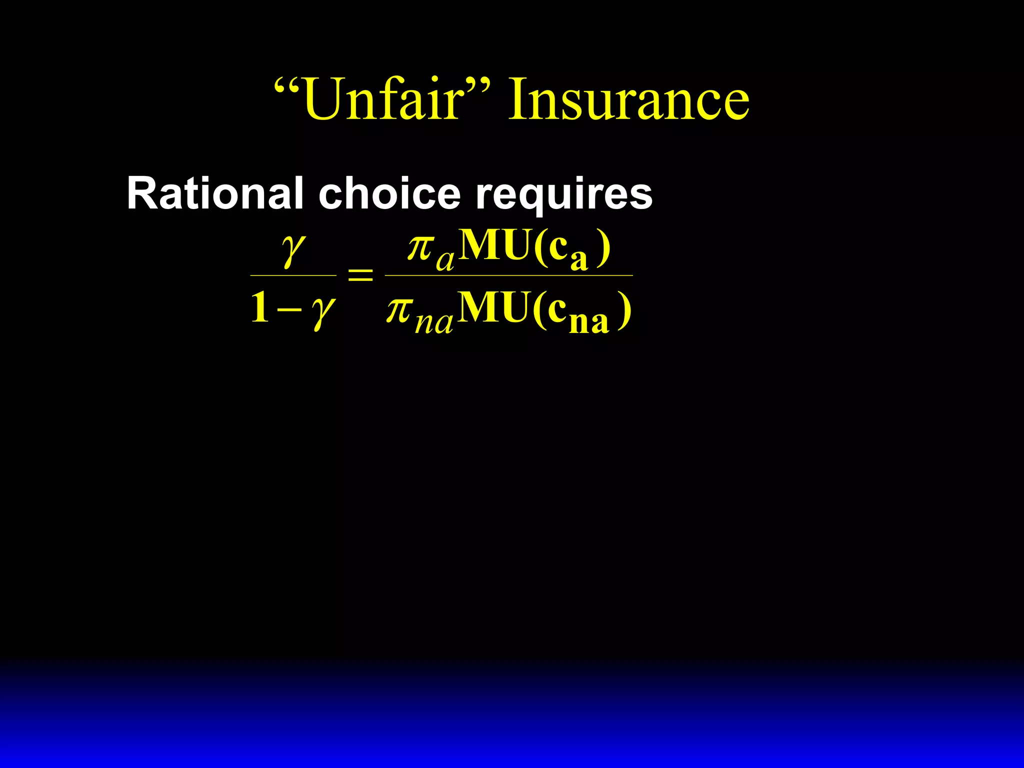
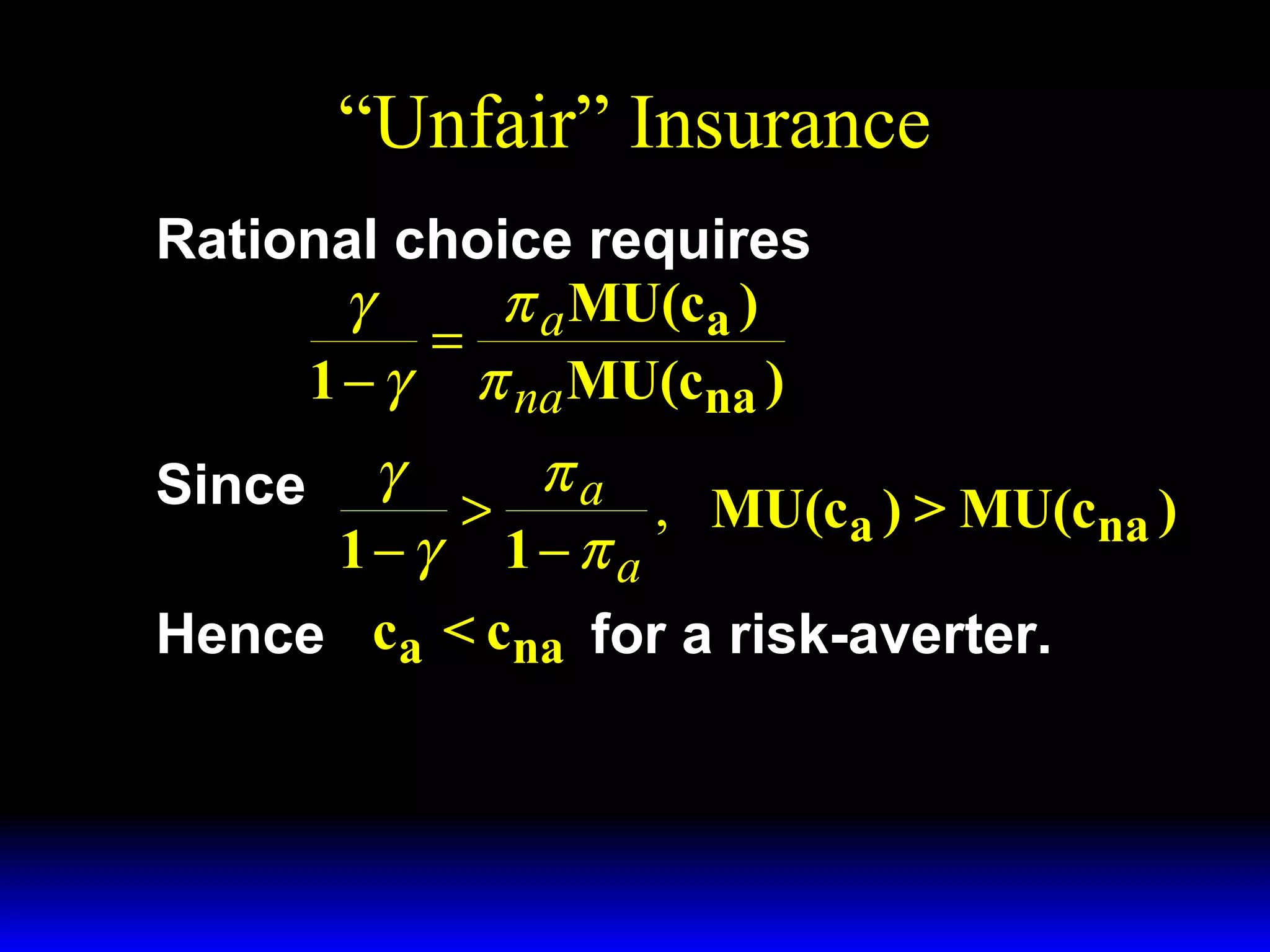
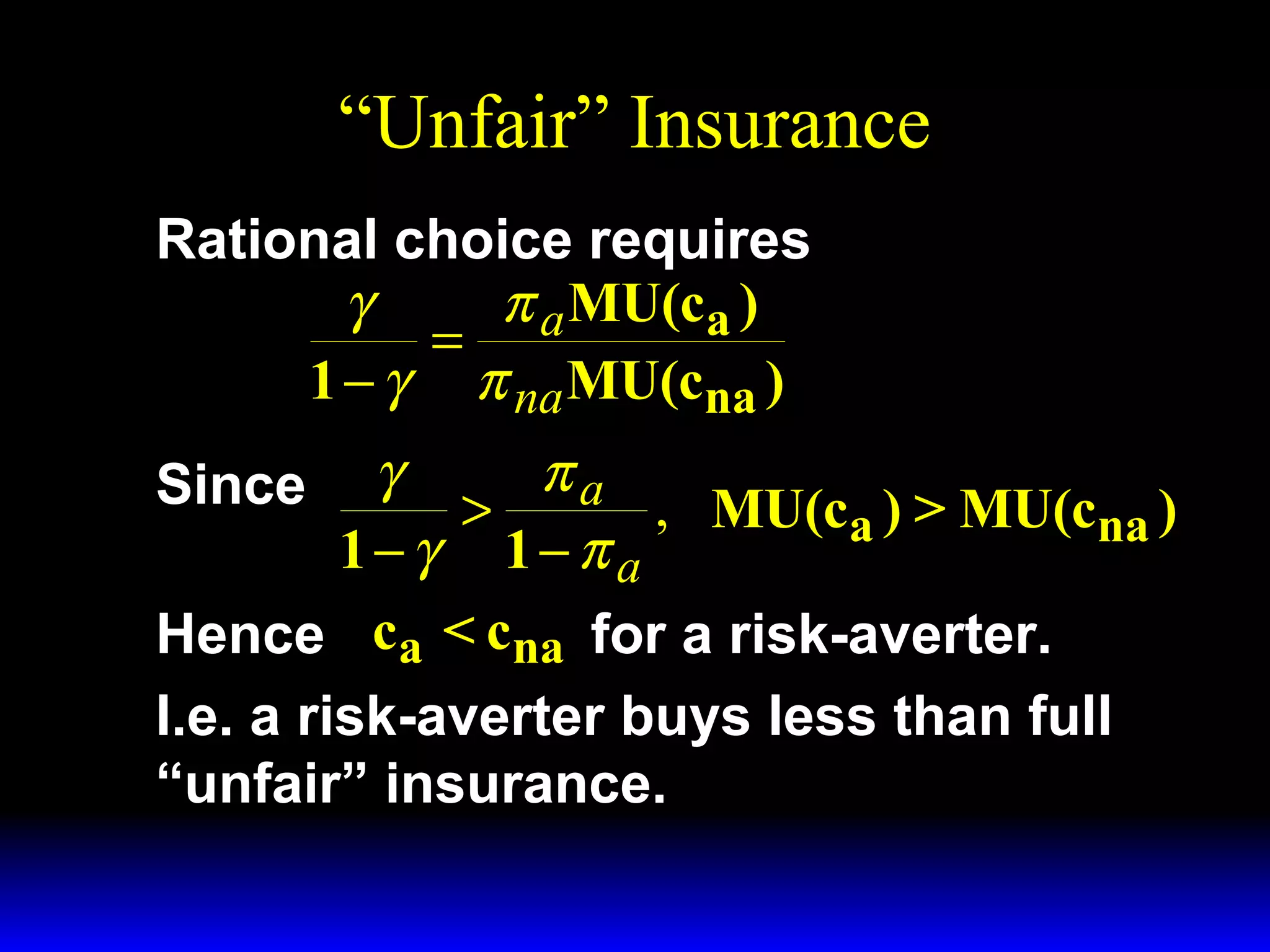
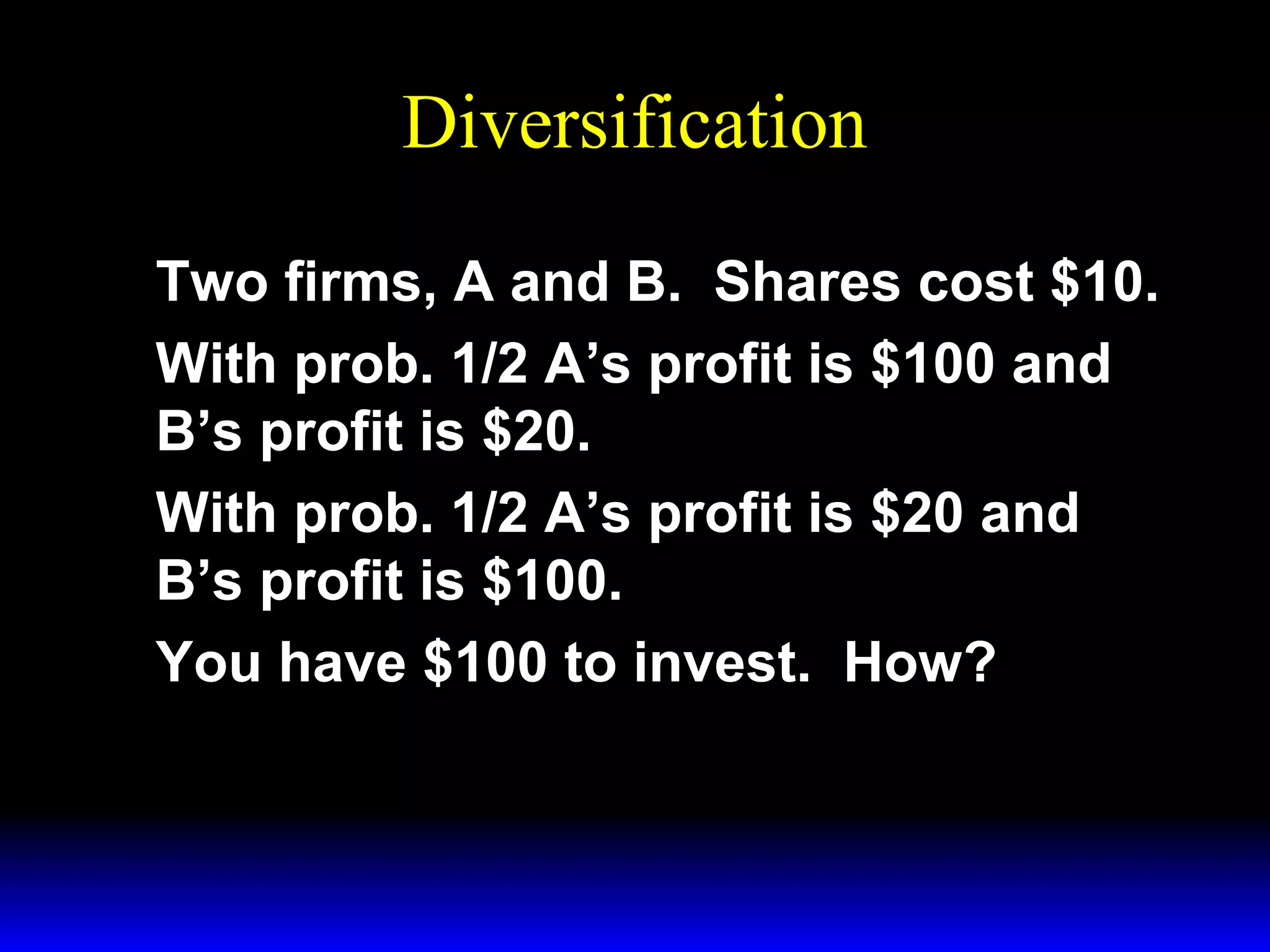
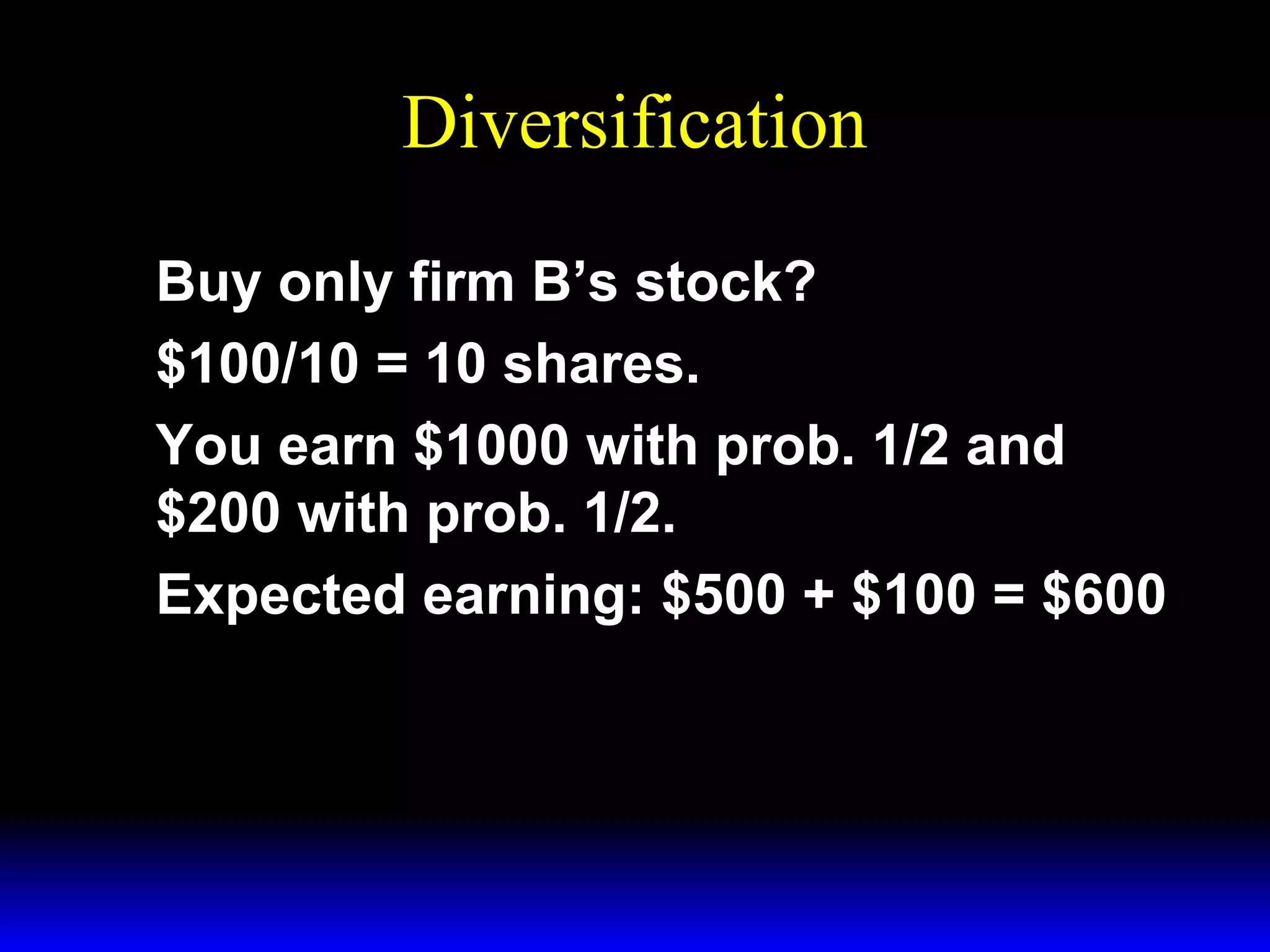
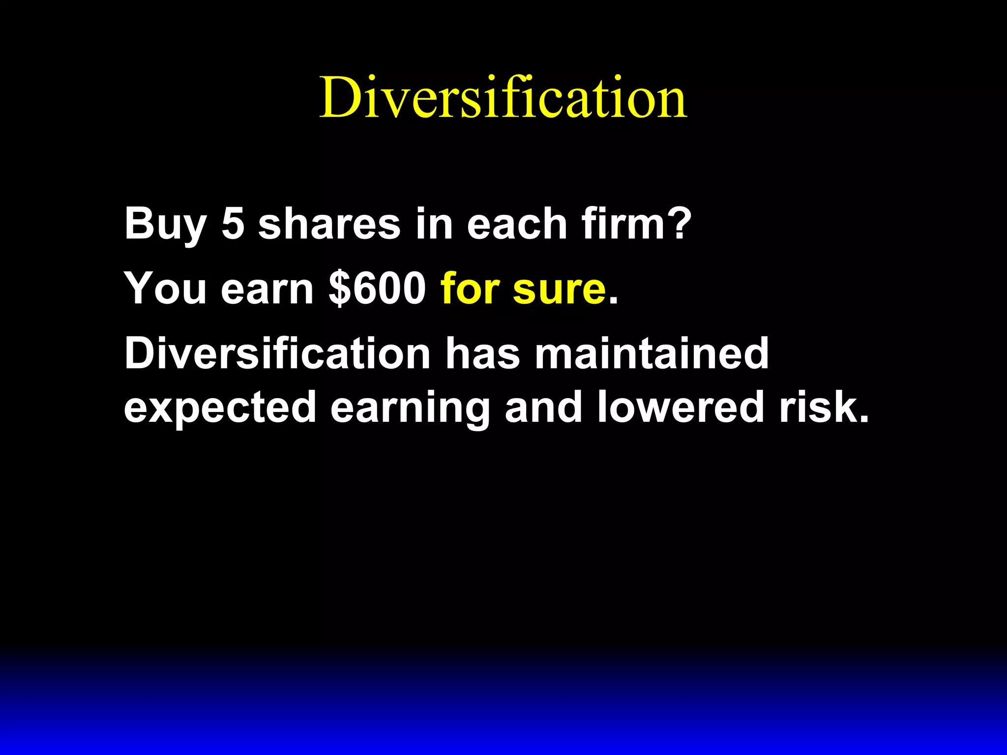
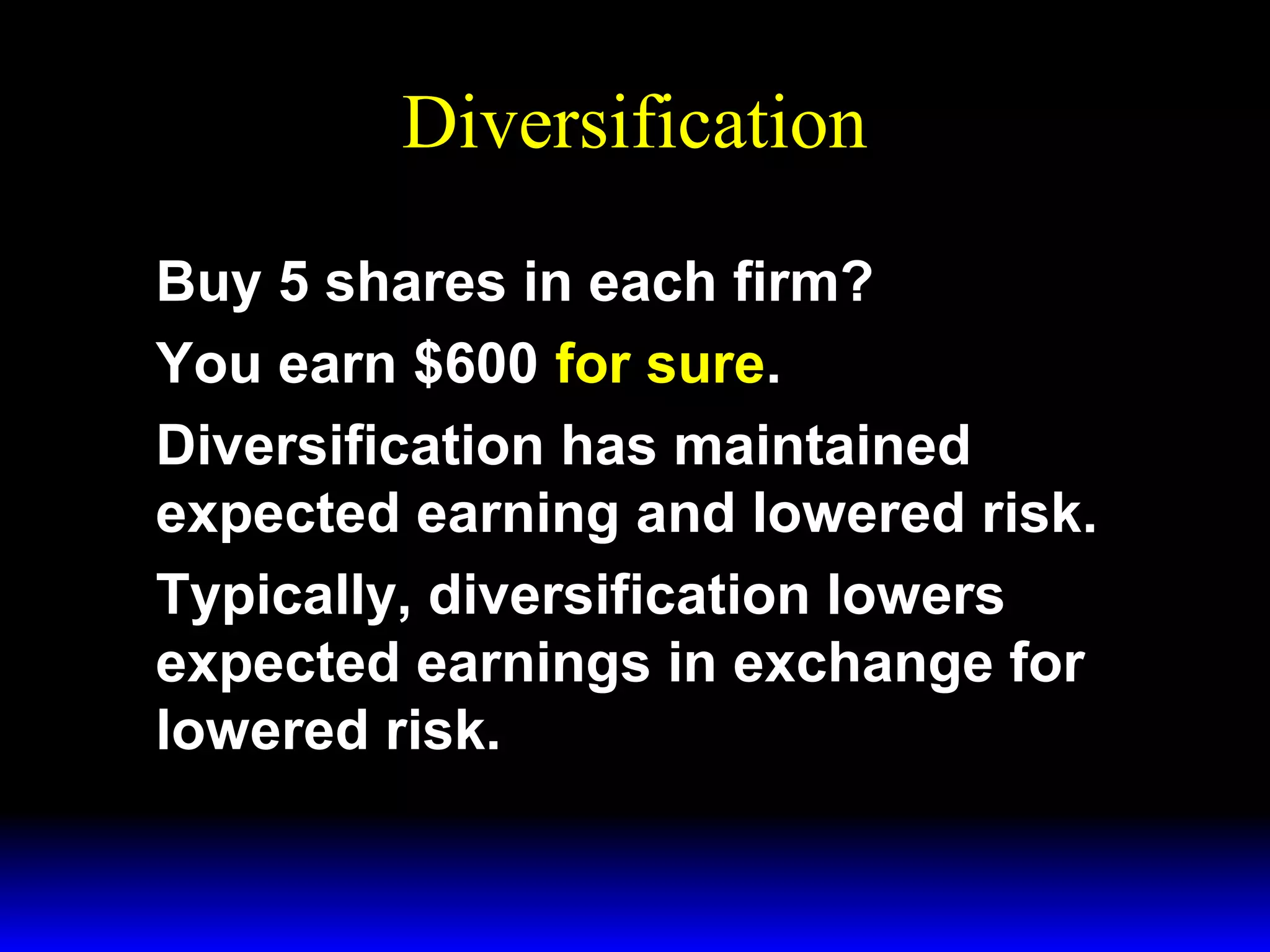
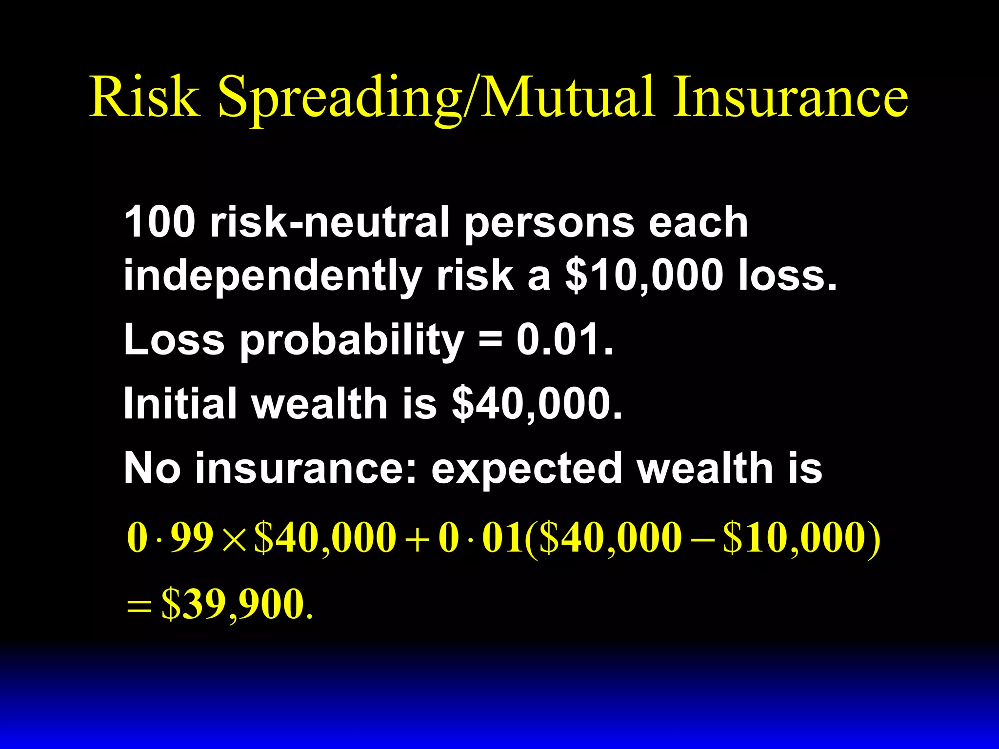
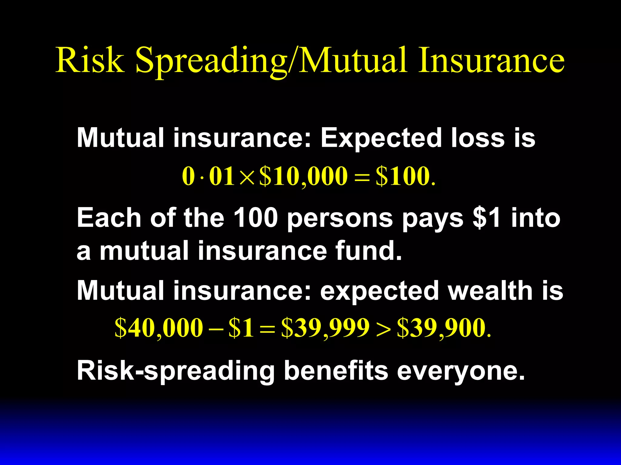
1. Chapter Twelve
Uncertainty

2. Uncertainty is Pervasive
What is uncertain in economic
systems?
– tomorrow’s prices
– future wealth
– future availability of commodities
– present and future actions of other
people.

3. Uncertainty is Pervasive
What are rational responses to
uncertainty?
– buying insurance (health, life,
auto)
– a portfolio of contingent
consumption goods.

4. States of Nature
Possible states of Nature:
– “car accident” (a)
– “no car accident” (na).
Accident occurs with probability π a,
does not with probability π na ;
π a + π na = 1.
Accident causes a loss of $L.

5. Contingencies
A contract implemented only when a
particular state of Nature occurs is
state-contingent.
E.g. the insurer pays only if there is
an accident.

6. Contingencies
A state-contingent consumption plan
is implemented only when a
particular state of Nature occurs.
E.g. take a vacation only if there is
no accident.

7. State-Contingent Budget
Constraints
Each $1 of accident insurance costs
γ.
Consumer has $m of wealth.
Cna is consumption value in the noaccident state.
Ca is consumption value in the
accident state.

8. State-Contingent Budget
Constraints
Cna
Ca

9. State-Contingent Budget
Constraints
Cna
A state-contingent consumption
with $17 consumption value in the
accident state and $20 consumption
value in the no-accident state.
20
17
Ca

10. State-Contingent Budget
Constraints
Without insurance,
Ca = m - L
Cna = m.

11. State-Contingent Budget
Constraints
Cna
m
The endowment bundle.
m−L
Ca

12. State-Contingent Budget
Constraints
Buy $K of accident insurance.
Cna = m - γK.
Ca = m - L - γK + K = m - L + (1- γ)K.

13. State-Contingent Budget
Constraints
Buy $K of accident insurance.
Cna = m - γK.
Ca = m - L - γK + K = m - L + (1- γ)K.
So K = (Ca - m + L)/(1- γ)

14. State-Contingent Budget
Constraints
Buy $K of accident insurance.
Cna = m - γK.
Ca = m - L - γK + K = m - L + (1- γ)K.
So K = (Ca - m + L)/(1- γ)
And Cna = m - γ (Ca - m + L)/(1- γ)

15. State-Contingent Budget
Constraints
Buy $K of accident insurance.
Cna = m - γK.
Ca = m - L - γK + K = m - L + (1- γ)K.
So K = (Ca - m + L)/(1- γ)
And Cna = m - γ (Ca - m + L)/(1- γ)
m − γL
γ
I.e. Cna = 1 − γ − 1 − γ Ca

16. State-Contingent Budget
Constraints
m − γL
γ
Cna =
−
Ca
1−γ
1−γ
Cna
m
The endowment bundle.
m−L
m − γL Ca
γ

17. State-Contingent Budget
Constraints
m − γL
γ
Cna =
−
Ca
1−γ
1−γ
Cna
m
The endowment bundle.
γ
slope = −
1−γ
m−L
m − γL Ca
γ

18. State-Contingent Budget
Constraints
m − γL
γ
Cna =
−
Ca
1−γ
1−γ
Cna
m
The endowment bundle.
γ
slope = −
1−γ
m−L
m − γL Ca
γ
Where is the
most preferred
state-contingent
consumption plan?

19. Preferences Under Uncertainty
Think of a lottery.
Win $90 with probability 1/2 and win
$0 with probability 1/2.
U($90) = 12, U($0) = 2.
Expected utility is

20. Preferences Under Uncertainty
Think of a lottery.
Win $90 with probability 1/2 and win
$0 with probability 1/2.
U($90) = 12, U($0) = 2.
Expected utility is
1
1
EU = × U($90) + × U($0)
2
2
1
1
= × 12 + × 2 = 7.
2
2

21. Preferences Under Uncertainty
Think of a lottery.
Win $90 with probability 1/2 and win
$0 with probability 1/2.
Expected money value of the lottery
is
1
1
EM = × $90 + × $0 = $45.
2
2

22. Preferences Under Uncertainty
EU = 7 and EM = $45.
U($45) > 7 ⇒ $45 for sure is
preferred to the lottery ⇒ riskaversion.
U($45) < 7 ⇒ the lottery is preferred
to $45 for sure ⇒ risk-loving.
U($45) = 7 ⇒ the lottery is preferred
equally to $45 for sure ⇒ riskneutrality.

23. Preferences Under Uncertainty
12
EU=7
2
$0
$45
$90
Wealth

24. Preferences Under Uncertainty
U($45) > EU ⇒ risk-aversion.
12
U($45)
EU=7
2
$0
$45
$90
Wealth

25. Preferences Under Uncertainty
U($45) > EU ⇒ risk-aversion.
12
U($45)
MU declines as wealth
rises.
EU=7
2
$0
$45
$90
Wealth

26. Preferences Under Uncertainty
12
EU=7
2
$0
$45
$90
Wealth

27. Preferences Under Uncertainty
U($45) < EU ⇒ risk-loving.
12
EU=7
U($45)
2
$0
$45
$90
Wealth

28. Preferences Under Uncertainty
U($45) < EU ⇒ risk-loving.
12
MU rises as wealth
rises.
EU=7
U($45)
2
$0
$45
$90
Wealth

29. Preferences Under Uncertainty
12
EU=7
2
$0
$45
$90
Wealth

30. Preferences Under Uncertainty
U($45) = EU ⇒ risk-neutrality.
12
U($45)=
EU=7
2
$0
$45
$90
Wealth

31. Preferences Under Uncertainty
U($45) = EU ⇒ risk-neutrality.
12
MU constant as wealth
rises.
U($45)=
EU=7
2
$0
$45
$90
Wealth

32. Preferences Under Uncertainty
State-contingent consumption plans
that give equal expected utility are
equally preferred.

33. Preferences Under Uncertainty
Cna
Indifference curves
EU1 < EU2 < EU3
EU3
EU2
EU1
Ca

34. Preferences Under Uncertainty
What is the MRS of an indifference
curve?
Get consumption c1 with prob. π 1 and
c2 with prob. π 2 (π 1 + π 2 = 1).
EU = π 1U(c1) + π 2U(c2).
For constant EU, dEU = 0.

35. Preferences Under Uncertainty
EU = π 1U(c1 ) + π 2U(c 2 )

36. Preferences Under Uncertainty
EU = π 1U(c1 ) + π 2U(c 2 )
dEU = π 1MU(c1 )dc1 + π 2MU(c 2 )dc 2

37. Preferences Under Uncertainty
EU = π 1U(c1 ) + π 2U(c 2 )
dEU = π 1MU(c1 )dc1 + π 2MU(c 2 )dc 2
dEU = 0 ⇒ π 1MU(c1 )dc1 + π 2MU(c 2 )dc 2 = 0

38. Preferences Under Uncertainty
EU = π 1U(c1 ) + π 2U(c 2 )
dEU = π 1MU(c1 )dc1 + π 2MU(c 2 )dc 2
dEU = 0 ⇒ π 1MU(c1 )dc1 + π 2MU(c 2 )dc 2 = 0
⇒ π 1MU(c1 )dc1 = −π 2MU(c 2 )dc 2

39. Preferences Under Uncertainty
EU = π 1U(c1 ) + π 2U(c 2 )
dEU = π 1MU(c1 )dc1 + π 2MU(c 2 )dc 2
dEU = 0 ⇒ π 1MU(c1 )dc1 + π 2MU(c 2 )dc 2 = 0
⇒ π 1MU(c1 )dc1 = −π 2MU(c 2 )dc 2
dc 2
π 1MU(c1 )
⇒
=−
.
dc1
π 2MU(c 2 )

40. Preferences Under Uncertainty
Cna
Indifference curves
EU1 < EU2 < EU3
dcna
π a MU(ca )
=−
dca
π na MU(cna )
EU3
EU2
EU1
Ca

41. Choice Under Uncertainty
Q: How is a rational choice made
under uncertainty?
A: Choose the most preferred
affordable state-contingent
consumption plan.

42. State-Contingent Budget
Constraints
m − γL
γ
Cna =
−
Ca
1−γ
1−γ
Cna
m
The endowment bundle.
γ
slope = −
1−γ
m−L
m − γL Ca
γ
Where is the
most preferred
state-contingent
consumption plan?

43. State-Contingent Budget
Constraints
m − γL
γ
Cna =
−
Ca
1−γ
1−γ
Cna
m
The endowment bundle.
γ
slope = −
1−γ
Affordable
plans
m−L
m − γL Ca
γ
Where is the
most preferred
state-contingent
consumption plan?

44. State-Contingent Budget
Constraints
Cna
More preferred
m
Where is the
most preferred
state-contingent
consumption plan?
m−L
m − γL Ca
γ

45. State-Contingent Budget
Constraints
Cna
Most preferred affordable plan
m
m−L
m − γL Ca
γ

46. State-Contingent Budget
Constraints
Cna
Most preferred affordable plan
m
m−L
m − γL Ca
γ

47. State-Contingent Budget
Constraints
Cna
Most preferred affordable plan
MRS = slope of budget
constraint
m
m−L
m − γL Ca
γ

48. State-Contingent Budget
Constraints
Cna
Most preferred affordable plan
MRS = slope of budget
constraint; i.e.
m
γ
π a MU(ca )
=
1 − γ π na MU(cna )
m−L
m − γL Ca
γ

49. Competitive Insurance
Suppose entry to the insurance
industry is free.
Expected economic profit = 0.
I.e. γK - π aK - (1 - π a)0 = (γ - π a)K = 0.
I.e. free entry ⇒ γ = π a.
If price of $1 insurance = accident
probability, then insurance is fair.

50. Competitive Insurance
When insurance is fair, rational
insurance choices satisfy
γ
πa
π a MU(ca )
=
=
1 − γ 1 − π a π na MU(cna )

51. Competitive Insurance
When insurance is fair, rational
insurance choices satisfy
γ
πa
π a MU(ca )
=
=
1 − γ 1 − π a π na MU(cna )
I.e. MU(ca ) = MU(cna )

52. Competitive Insurance
When insurance is fair, rational
insurance choices satisfy
γ
πa
π a MU(ca )
=
=
1 − γ 1 − π a π na MU(cna )
I.e. MU(ca ) = MU(cna )
Marginal utility of income must be
the same in both states.

53. Competitive Insurance
How much fair insurance does a riskaverse consumer buy?
MU(ca ) = MU(cna )

54. Competitive Insurance
How much fair insurance does a riskaverse consumer buy?
MU(ca ) = MU(cna )
Risk-aversion ⇒ MU(c) ↓ as c ↑.

55. Competitive Insurance
How much fair insurance does a riskaverse consumer buy?
MU(ca ) = MU(cna )
Risk-aversion ⇒ MU(c) ↓ as c ↑.
Hence ca = cna .

56. Competitive Insurance
How much fair insurance does a riskaverse consumer buy?
MU(ca ) = MU(cna )
Risk-aversion ⇒ MU(c) ↓ as c ↑.
Hence ca = cna .
I.e. full-insurance.

57. “Unfair” Insurance
Suppose insurers make positive
expected economic profit.
I.e. γK - π aK - (1 - π a)0 = (γ - π a)K > 0.

58. “Unfair” Insurance
Suppose insurers make positive
expected economic profit.
I.e. γK - π aK - (1 - π a)0 = (γ - π a)K > 0.
Then ⇒ γ > π a ⇒ γ > π a .
1−γ 1−πa

59. “Unfair” Insurance
Rational choice requires
γ
π a MU(ca )
=
1 − γ π na MU(cna )

60. “Unfair” Insurance
Rational choice requires
γ
π a MU(ca )
=
1 − γ π na MU(cna )
Since
γ
πa
>
, MU(ca ) > MU(cna )
1−γ 1−πa

61. “Unfair” Insurance
Rational choice requires
γ
π a MU(ca )
=
1 − γ π na MU(cna )
γ
πa
>
, MU(ca ) > MU(cna )
1−γ 1−πa
Hence ca < cna for a risk-averter.
Since

62. “Unfair” Insurance
Rational choice requires
γ
π a MU(ca )
=
1 − γ π na MU(cna )
γ
πa
>
, MU(ca ) > MU(cna )
1−γ 1−πa
Hence ca < cna for a risk-averter.
I.e. a risk-averter buys less than full
“unfair” insurance.
Since

63. Uncertainty is Pervasive
What are rational responses to
uncertainty?
– buying insurance (health, life,
auto)
– a portfolio of contingent
consumption goods.

64. Uncertainty is Pervasive
What are rational responses to
uncertainty?
 – buying insurance (health, life,
auto)
– a portfolio of contingent
consumption goods.

65. Uncertainty is Pervasive
What are rational responses to
uncertainty?
 – buying insurance (health, life,
auto)
?
– a portfolio of contingent
consumption goods.

66. Diversification
Two firms, A and B. Shares cost $10.
With prob. 1/2 A’s profit is $100 and
B’s profit is $20.
With prob. 1/2 A’s profit is $20 and
B’s profit is $100.
You have $100 to invest. How?

67. Diversification
Buy only firm A’s stock?
$100/10 = 10 shares.
You earn $1000 with prob. 1/2 and
$200 with prob. 1/2.
Expected earning: $500 + $100 = $600

68. Diversification
Buy only firm B’s stock?
$100/10 = 10 shares.
You earn $1000 with prob. 1/2 and
$200 with prob. 1/2.
Expected earning: $500 + $100 = $600

69. Diversification
Buy 5 shares in each firm?
You earn $600 for sure.
Diversification has maintained
expected earning and lowered risk.

70. Diversification
Buy 5 shares in each firm?
You earn $600 for sure.
Diversification has maintained
expected earning and lowered risk.
Typically, diversification lowers
expected earnings in exchange for
lowered risk.

71. Risk Spreading/Mutual Insurance
100 risk-neutral persons each
independently risk a $10,000 loss.
Loss probability = 0.01.
Initial wealth is $40,000.
No insurance: expected wealth is
0 ⋅ 99 × $40,000 + 0 ⋅ 01($40,000 − $10,000)
= $39,900.

72. Risk Spreading/Mutual Insurance
Mutual insurance: Expected loss is
0 ⋅ 01 × $10,000 = $100.
Each of the 100 persons pays $1 into
a mutual insurance fund.
Mutual insurance: expected wealth is
$40,000 − $1 = $39,999 > $39,900.
Risk-spreading benefits everyone.