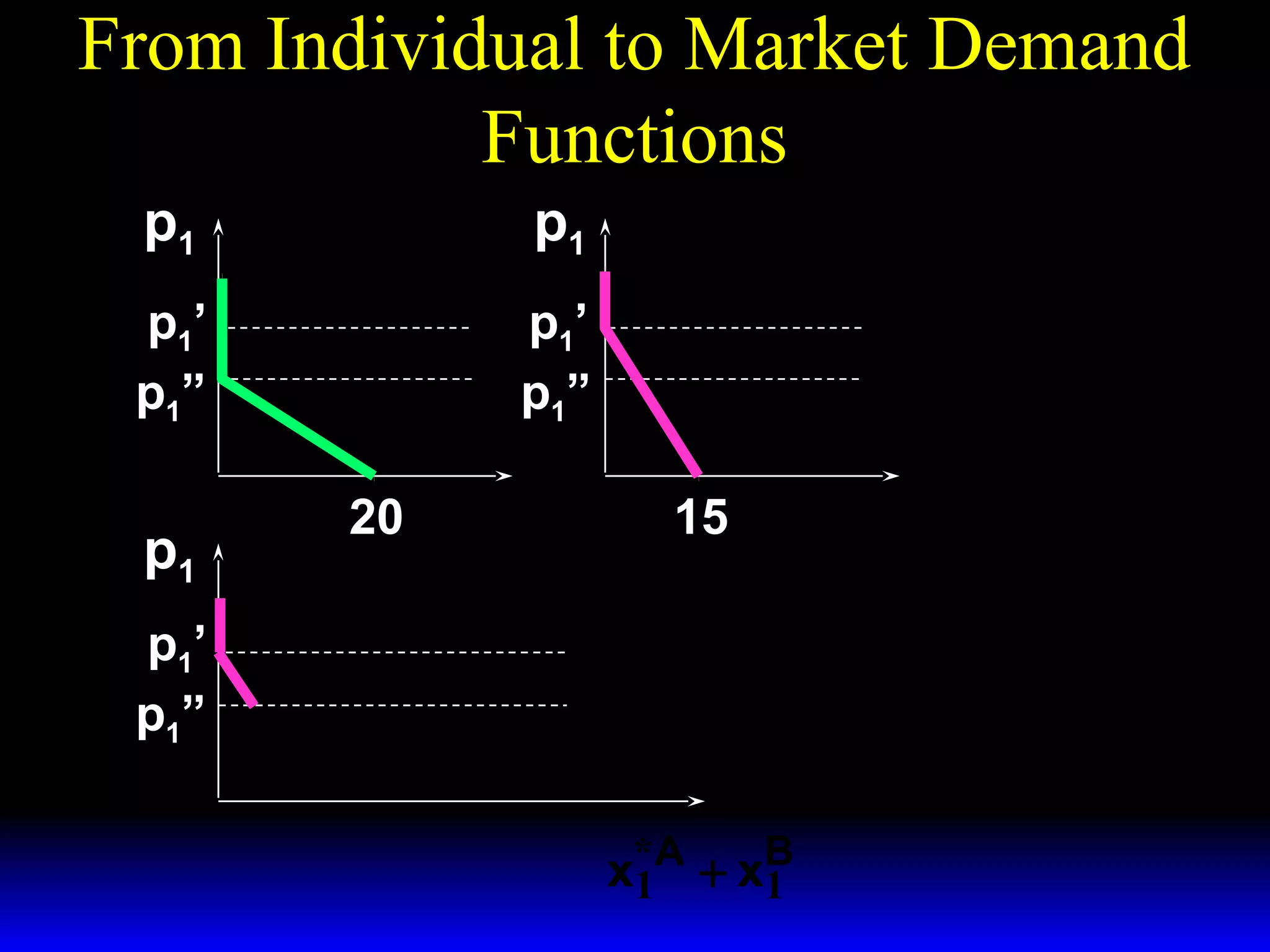
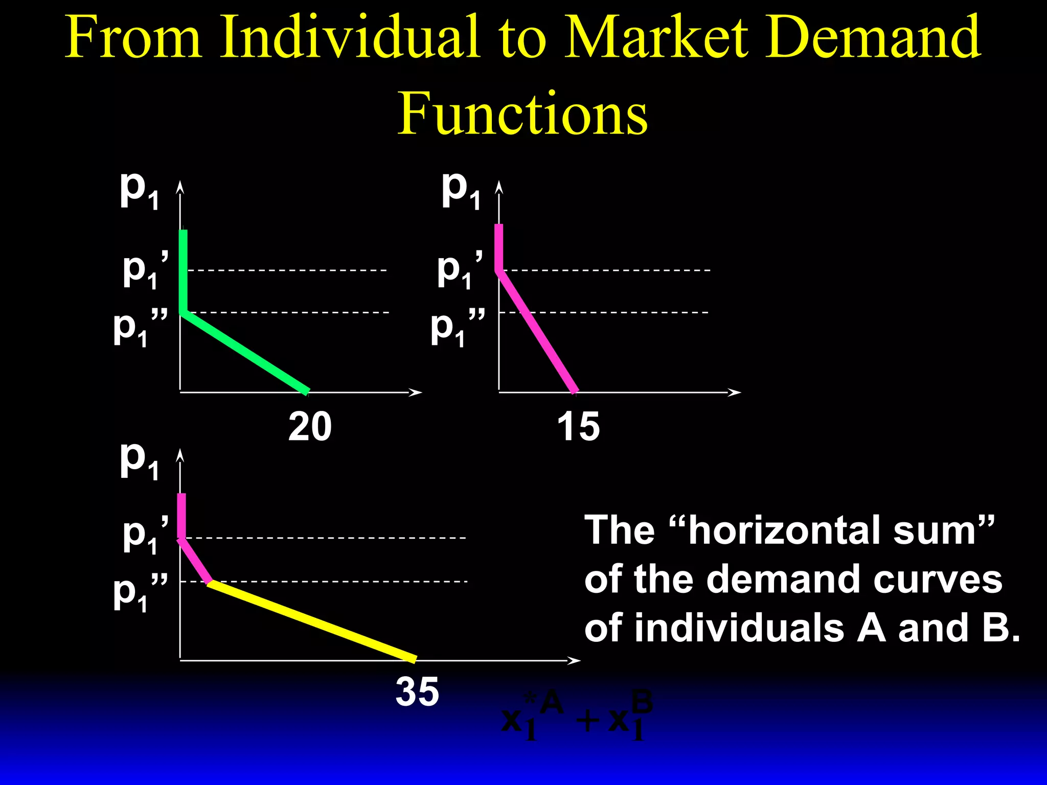
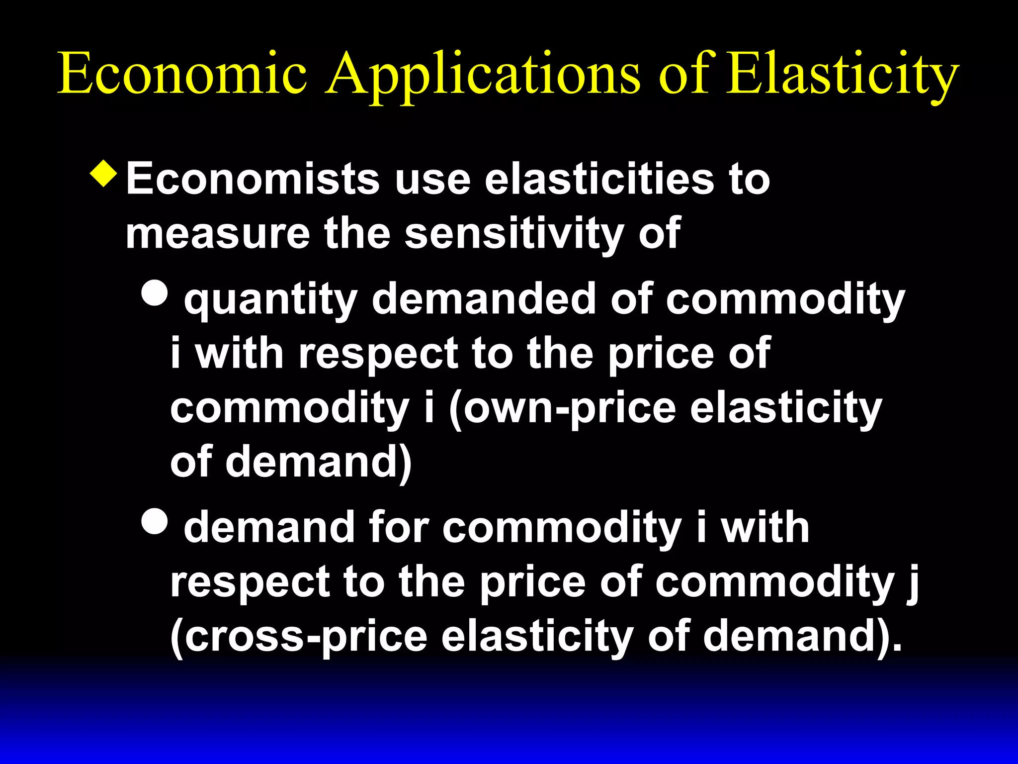
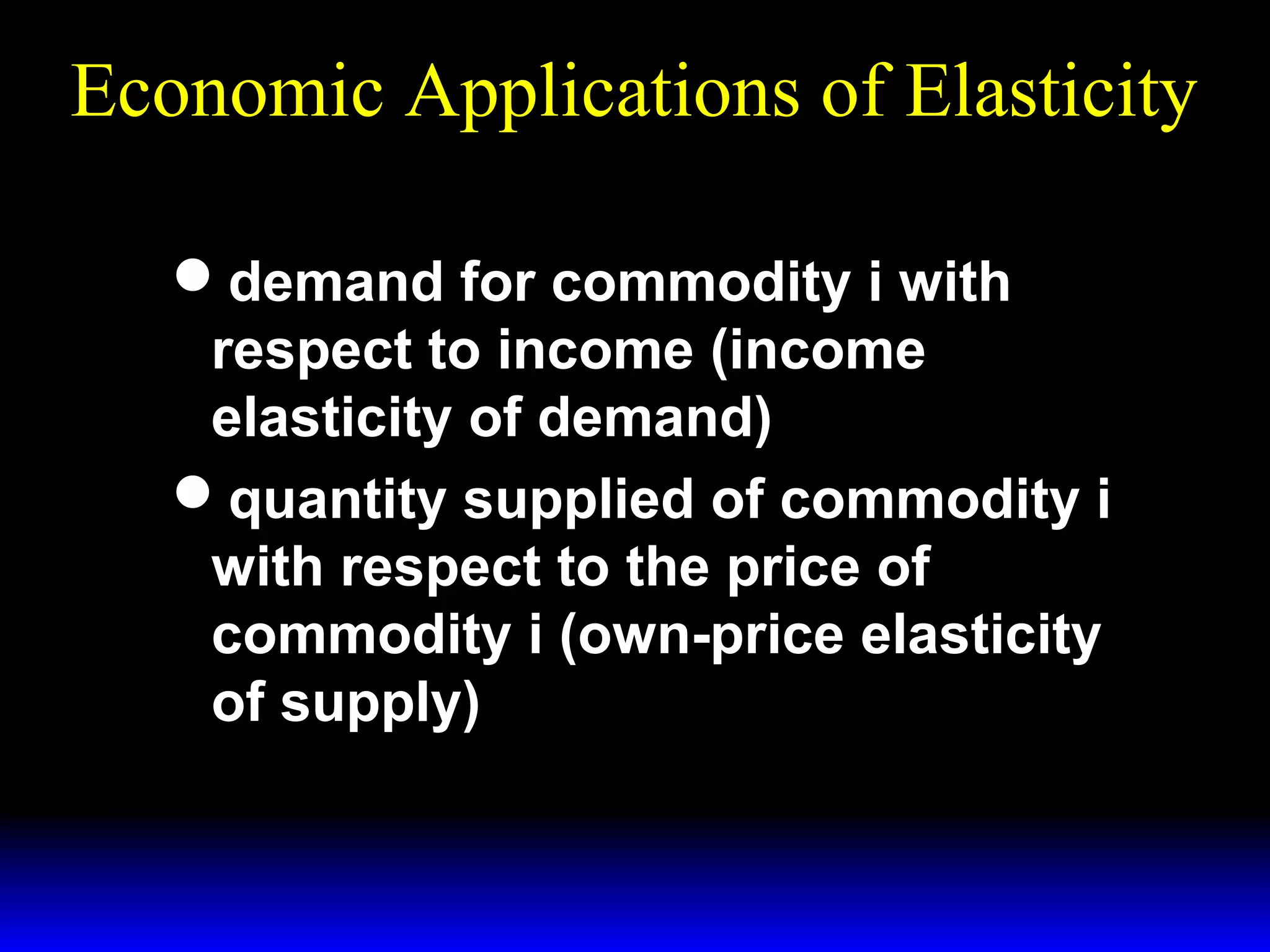
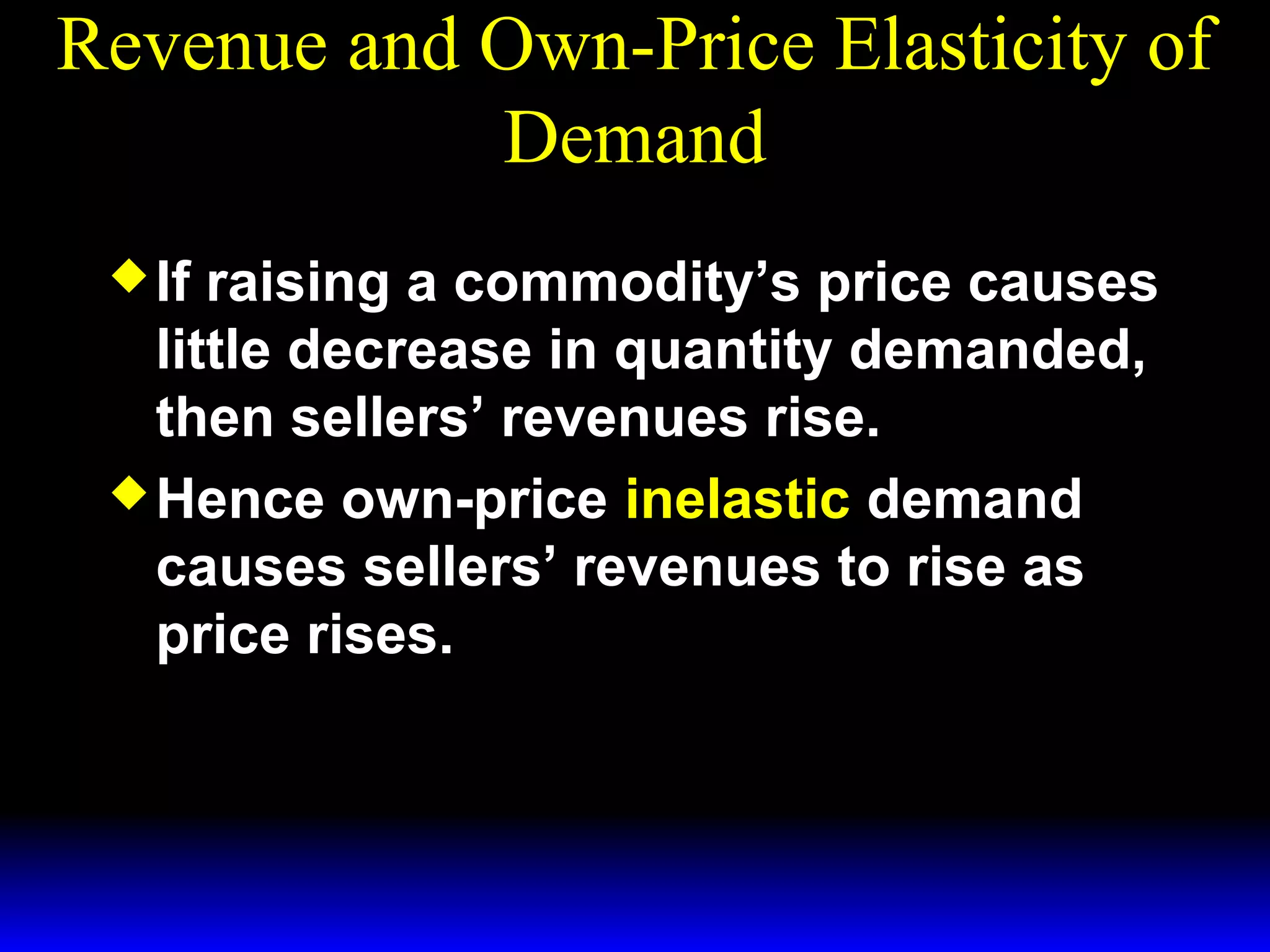
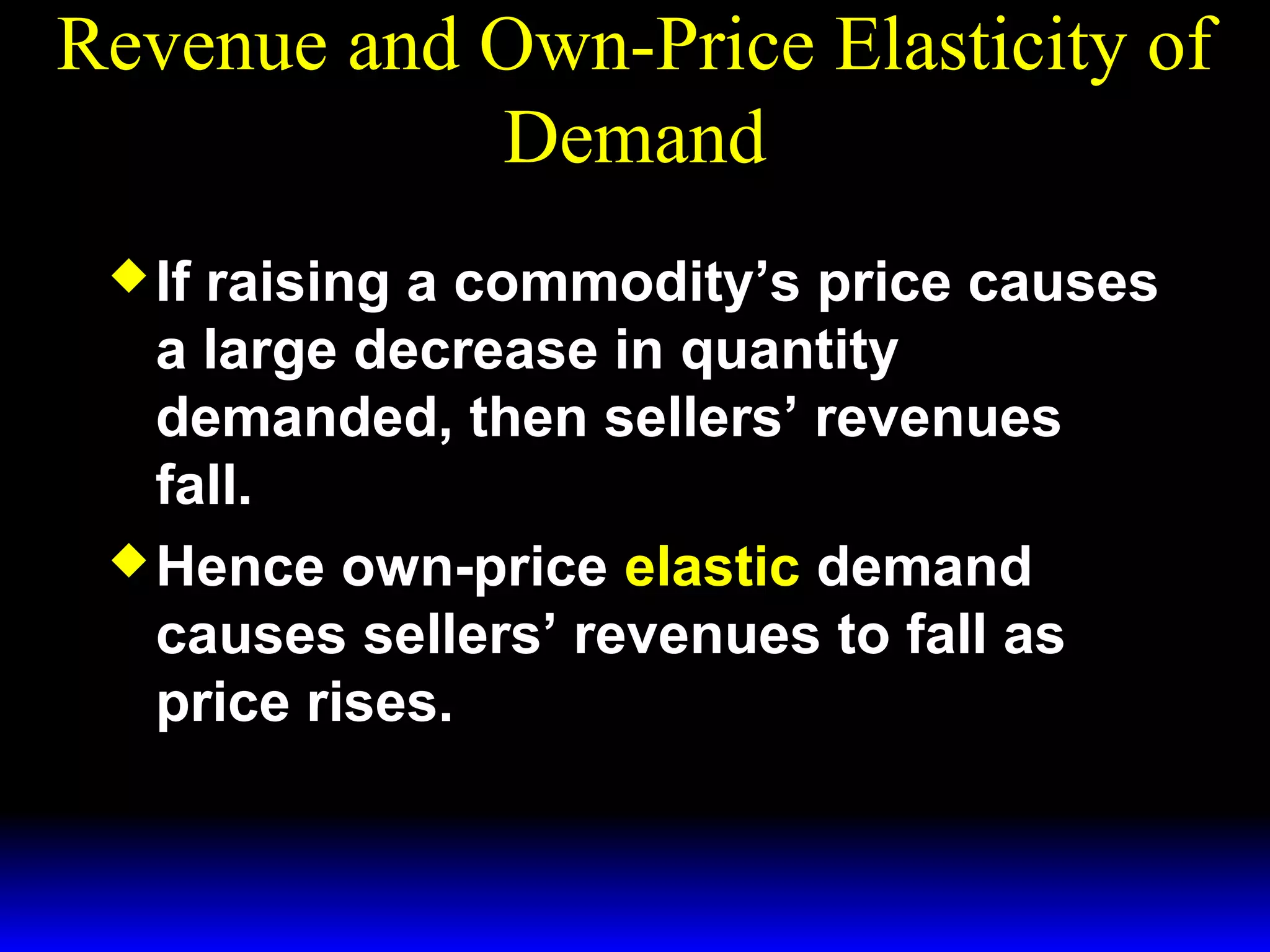
This document discusses the concept of market demand and how it relates to individual consumer demand. It explains that the market demand curve is the horizontal sum of individual demand curves. It then discusses the concept of elasticity, including own-price elasticity of demand and how elasticity measures the sensitivity of one variable to changes in another. It provides examples of how own-price elasticity can be calculated using demand curves and formulas. It also discusses how the elasticity measurement relates to whether raising price will increase or decrease seller revenue.

1. Chapter Fifteen
Market Demand

2. From Individual to Market Demand
Functions
 Think
of an economy containing n
consumers, denoted by i = 1, … ,n.
 Consumer i’s ordinary demand
function for commodity j is
x*i (p1 , p 2 , mi )
j

3. From Individual to Market Demand
Functions
 When
all consumers are price-takers,
the market demand function for
commodity j is
n *i
X j ( p1 , p 2 , m ,, m ) = ∑ x j (p1 , p 2 , mi ).
i= 1
1
 If
n
all consumers are identical then
X j ( p1 , p 2 , M) = n × x* ( p1 , p 2 , m)
j
where M = nm.

4. From Individual to Market Demand
Functions
 The
market demand curve is the
“horizontal sum” of the individual
consumers’ demand curves.
 E.g. suppose there are only two
consumers; i = A,B.

5. From Individual to Market Demand
Functions
p1
p1
p1’
p1”
p1’
p1”
20 x*A
1
15
x*B
1

6. From Individual to Market Demand
Functions
p1
p1
p1’
p1”
p1’
p1”
p1
20 x*A
1
15
p1’
x*A + xB
1
1
x*B
1

7. From Individual to Market Demand
Functions
p1
p1
p1’
p1”
p1’
p1”
p1
20 x*A
1
15
p1’
p1”
x*A + xB
1
1
x*B
1

8. From Individual to Market Demand
Functions
p1
p1
p1’
p1”
p1’
p1”
p1
20 x*A
1
15
x*B
1
The “horizontal sum”
of the demand curves
of individuals A and B.
p1’
p1”
35
x*A + xB
1
1

9. Elasticities
 Elasticity
measures the “sensitivity”
of one variable with respect to
another.
 The elasticity of variable X with
respect to variable Y is
% ∆x
ε x,y =
.
% ∆y

10. Economic Applications of Elasticity
 Economists
use elasticities to
measure the sensitivity of
quantity demanded of commodity
i with respect to the price of
commodity i (own-price elasticity
of demand)
demand for commodity i with
respect to the price of commodity j
(cross-price elasticity of demand).

11. Economic Applications of Elasticity
demand for commodity i with
respect to income (income
elasticity of demand)
quantity supplied of commodity i
with respect to the price of
commodity i (own-price elasticity
of supply)

12. Economic Applications of Elasticity
quantity supplied of commodity i
with respect to the wage rate
(elasticity of supply with respect to
the price of labor)
and many, many others.

13. Own-Price Elasticity of Demand
 Q:
Why not use a demand curve’s
slope to measure the sensitivity of
quantity demanded to a change in a
commodity’s own price?

14. Own-Price Elasticity of Demand
p1
10
slope
=-2
5
p1
10
X1*
slope
= - 0.2
50 X *
1
In which case is the quantity demanded
X1* more sensitive to changes to p1?

15. Own-Price Elasticity of Demand
p1
10
slope
=-2
5
p1
10
X1*
slope
= - 0.2
50 X *
1
In which case is the quantity demanded
X1* more sensitive to changes to p1?

16. Own-Price Elasticity of Demand
p1
10
10-packs
slope
=-2
5
p1
10
X1*
Single Units
slope
= - 0.2
50 X *
1
In which case is the quantity demanded
X1* more sensitive to changes to p1?

17. Own-Price Elasticity of Demand
p1
10
10-packs
slope
=-2
5
p1
10
X1*
Single Units
slope
= - 0.2
50 X *
1
In which case is the quantity demanded
X1* more sensitive to changes to p1?
It is the same in both cases.

18. Own-Price Elasticity of Demand
 Q:
Why not just use the slope of a
demand curve to measure the
sensitivity of quantity demanded to a
change in a commodity’s own price?
 A: Because the value of sensitivity
then depends upon the (arbitrary)
units of measurement used for
quantity demanded.

19. Own-Price Elasticity of Demand
*
% ∆ x1
ε *
=
x1 ,p1 % ∆p
1
is a ratio of percentages and so has no
units of measurement.
Hence own-price elasticity of demand is
a sensitivity measure that is independent
of units of measurement.

20. Arc and Point Elasticities
 An
“average” own-price elasticity of
demand for commodity i over an
interval of values for pi is an arcelasticity, usually computed by a
mid-point formula.
 Elasticity computed for a single
value of pi is a point elasticity.

21. Arc Own-Price Elasticity
pi
pi’+h
p i’
pi’-h
What is the “average” own-price
elasticity of demand for prices
in an interval centered on pi’?
X i*

22. Arc Own-Price Elasticity
pi
pi’+h
p i’
pi’-h
What is the “average” own-price
elasticity of demand for prices
in an interval centered on pi’?
Xi"
Xi '"
X i*

23. Arc Own-Price Elasticity
pi
pi’+h
p i’
pi’-h
What is the “average” own-price
elasticity of demand for prices
in an interval centered on pi’?
% ∆X*
i
ε * =
Xi ,pi
% ∆pi
Xi"
Xi '"
X i*

24. Arc Own-Price Elasticity
pi
pi’+h
p i’
pi’-h
What is the “average” own-price
elasticity of demand for prices
in an interval centered on pi’?
% ∆X*
i
ε * =
Xi ,pi
% ∆pi
Xi"
2h
% ∆pi = 100 ×
pi '
Xi '"
X i*

25. Arc Own-Price Elasticity
pi
pi’+h
p i’
pi’-h
What is the “average” own-price
elasticity of demand for prices
in an interval centered on pi’?
% ∆X*
i
ε * =
Xi ,pi
% ∆pi
Xi"
2h
% ∆pi = 100 ×
pi '
Xi '"
X i*
% ∆X* = 100 ×
i
( Xi"− Xi '")
( Xi"+ Xi '") / 2

26. Arc Own-Price Elasticity
*
% ∆Xi
ε * =
Xi ,pi
% ∆pi
2h
% ∆pi = 100 ×
pi '
% ∆X* = 100 ×
i
( Xi"− Xi '")
( Xi"+ Xi '") / 2

27. Arc Own-Price Elasticity
*
% ∆Xi
ε * =
Xi ,pi
% ∆pi
2h
% ∆pi = 100 ×
pi '
% ∆X* = 100 ×
i
( Xi"− Xi '")
( Xi"+ Xi '") / 2
So
%∆X*
pi '
( Xi "− Xi '" )
i =
ε X* ,p =
×
.
i i
%∆pi ( Xi "+ Xi '" ) / 2
2h
is the arc own-price elasticity of demand.

28. Point Own-Price Elasticity
What is the own-price elasticity
of demand in a very small interval
of prices centered on pi’?
pi
pi’+h
p i’
pi’-h
Xi"
Xi '"
X i*
%∆X*
pi '
( Xi "− Xi '" )
i =
ε X* ,p =
×
.
i i
%∆pi ( Xi "+ Xi '" ) / 2
2h

29. Point Own-Price Elasticity
What is the own-price elasticity
of demand in a very small interval
of prices centered on pi’?
As h → 0,
pi
pi’+h
p i’
pi’-h
Xi"
Xi '"
X i*
%∆X*
pi '
( Xi "− Xi '" )
i =
ε X* ,p =
×
.
i i
%∆pi ( Xi "+ Xi '" ) / 2
2h

30. Point Own-Price Elasticity
pi
pi’+h
p i’
pi’-h
What is the own-price elasticity
of demand in a very small interval
of prices centered on pi’?
As h → 0,
Xi" Xi '"
X i*
%∆X*
pi '
( Xi "− Xi '" )
i =
ε X* ,p =
×
.
i i
%∆pi ( Xi "+ Xi '" ) / 2
2h

31. Point Own-Price Elasticity
pi
pi’+h
p i’
pi’-h
What is the own-price elasticity
of demand in a very small interval
of prices centered on pi’?
As h → 0,
Xi '
X i*
%∆X*
pi '
( Xi "− Xi '" )
i =
ε X* ,p =
×
.
i i
%∆pi ( Xi "+ Xi '" ) / 2
2h

32. Point Own-Price Elasticity
pi
p i’
What is the own-price elasticity
of demand in a very small interval
of prices centered on pi’?
As h → 0,
pi ' dX*
i
ε * →
×
Xi ,pi
Xi ' dpi
Xi '
X i*
%∆X*
pi '
( Xi "− Xi '" )
i =
ε X* ,p =
×
.
i i
%∆pi ( Xi "+ Xi '" ) / 2
2h

33. Point Own-Price Elasticity
pi
p i’
What is the own-price elasticity
of demand in a very small interval
of prices centered on pi’?
*
pi ' dXi
ε * =
×
Xi ,pi
Xi ' dpi
is the elasticity at the
point ( Xi ', pi ' ).
Xi '
X i*

34. Point Own-Price Elasticity
dX*
i
ε * =
×
Xi ,pi
X* dpi
i
pi
E.g. Suppose pi = a - bXi.
Then Xi = (a-pi)/b and
*
dXi
1
= − . Therefore,
dpi
b
pi
 − 1  = − pi .
εX* ,p =
×

i
i
( a − pi ) / b  b
a − pi

35. Point Own-Price Elasticity
pi
pi = a - bXi*
a
a/b
Xi*

36. Point Own-Price Elasticity
pi
pi = a - bXi*
pi
εX* ,p = −
i
i
a − pi
a
a/b
Xi*

37. Point Own-Price Elasticity
pi
a
pi = a - bXi*
pi
εX* ,p = −
i
i
a − pi
p = 0 ⇒ε = 0
a/b
Xi*

38. Point Own-Price Elasticity
pi
a
pi
εX* ,p = −
i
i
a − pi
pi = a - bXi*
p = 0 ⇒ε = 0
ε =0
a/b
Xi*

39. Point Own-Price Elasticity
pi
a
pi
εX* ,p = −
i
i
a − pi
pi = a - bXi*
a
a/2
p = ⇒ε = −
= −1
2
a −a / 2
ε =0
a/b
Xi*

40. Point Own-Price Elasticity
pi
a
a/2
pi
εX* ,p = −
i
i
a − pi
pi = a - bXi*
a
a/2
p = ⇒ε = −
= −1
2
a −a / 2
ε = −1
ε =0
a/2b
a/b
Xi*

41. Point Own-Price Elasticity
pi
a
a/2
pi
εX* ,p = −
i
i
a − pi
pi = a - bXi*
a
p = a ⇒ε = −
= −∞
a −a
ε = −1
ε =0
a/2b
a/b
Xi*

42. Point Own-Price Elasticity
pi = a - bXi*
pi
a ε = −∞
a/2
pi
εX* ,p = −
i
i
a − pi
a
p = a ⇒ε = −
= −∞
a −a
ε = −1
ε =0
a/2b
a/b
Xi*

43. Point Own-Price Elasticity
pi
pi
εX* ,p = −
i
i
a − pi
pi = a - bXi*
a ε = −∞
own-price elastic
a/2
ε = −1
own-price inelastic
ε =0
a/2b
a/b
Xi*

44. Point Own-Price Elasticity
pi
pi
εX* ,p = −
i
i
a − pi
pi = a - bXi*
a ε = −∞
own-price elastic
a/2
ε = −1 (own-price unit elastic)
own-price inelastic
ε =0
a/2b
a/b
Xi*

45. Point Own-Price Elasticity
dX*
i
ε * =
×
Xi ,pi
X* dpi
i
pi
E.g.
so
X* = kpia .
i
Then
dX*
i = apa −1
i
dpi
a
pi
pi
a −1
εX* ,p = a × kapi
=a
= a.
a
i
i
kpi
pi

46. Point Own-Price Elasticity
pi
k
*
a
−2
Xi = kpi = kpi =
2
pi
ε = −2 everywhere along
the demand curve.
X i*

47. Revenue and Own-Price Elasticity of
Demand
 If
raising a commodity’s price causes
little decrease in quantity demanded,
then sellers’ revenues rise.
 Hence own-price inelastic demand
causes sellers’ revenues to rise as
price rises.

48. Revenue and Own-Price Elasticity of
Demand
 If
raising a commodity’s price causes
a large decrease in quantity
demanded, then sellers’ revenues
fall.
 Hence own-price elastic demand
causes sellers’ revenues to fall as
price rises.

49. Revenue and Own-Price Elasticity of
Demand
R( p ) = p × X* (p ).
Sellers’ revenue is

50. Revenue and Own-Price Elasticity of
Demand
R( p ) = p × X* (p ).
Sellers’ revenue is
dR
dX*
So
= X* (p ) + p
dp
dp

51. Revenue and Own-Price Elasticity of
Demand
R( p ) = p × X* (p ).
Sellers’ revenue is
dR
dX*
So
= X* (p ) + p
dp
dp
*

p dX
*
= X (p )1 +

*
 X (p ) dp 



52. Revenue and Own-Price Elasticity of
Demand
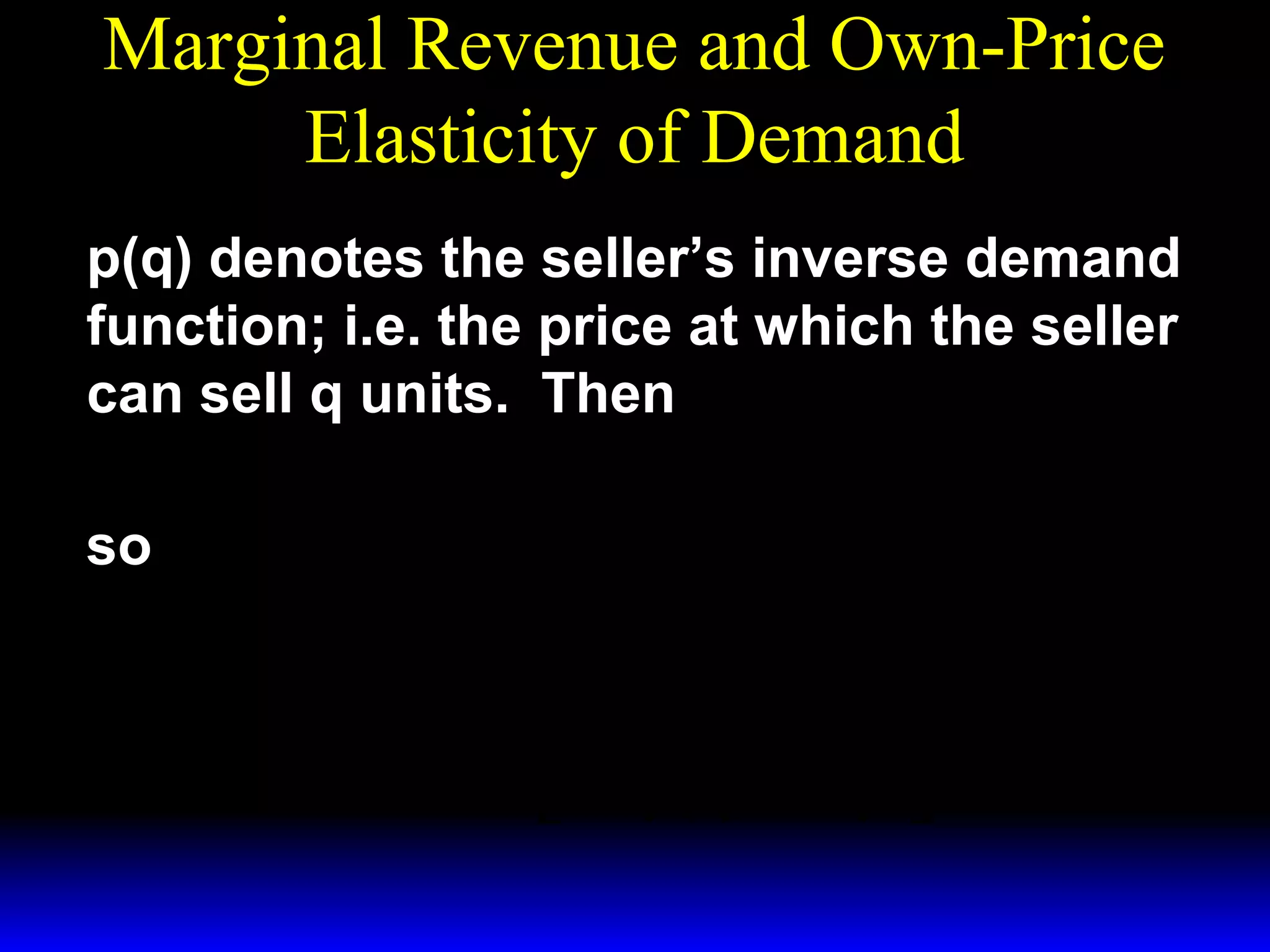
R( p ) = p × X* (p ).
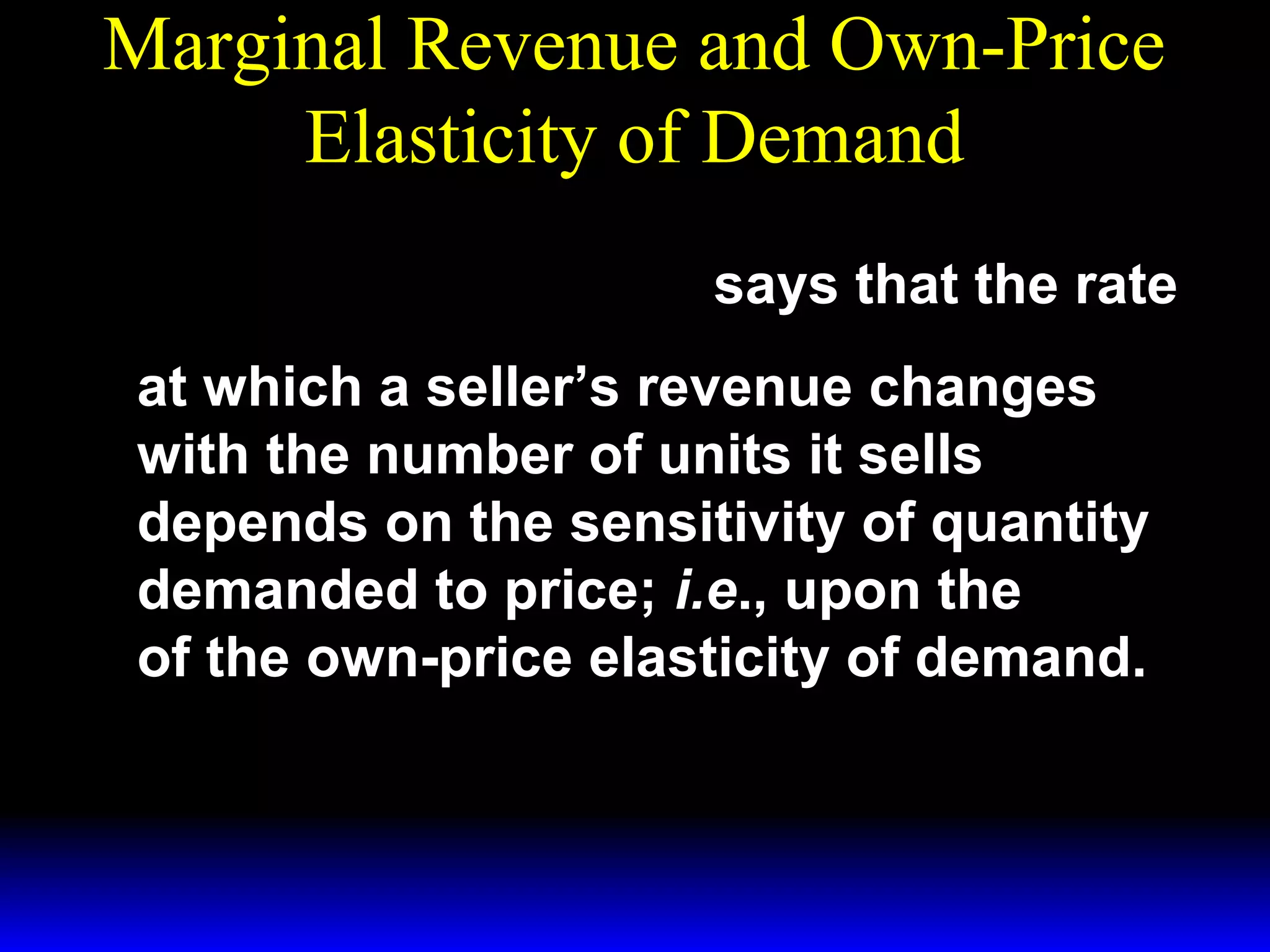
Sellers’ revenue is
dR
dX*
So
= X* (p ) + p
dp
dp
*

p dX
*
= X (p )1 +

*
 X (p ) dp 


= X* (p )[ 1 + ε ] .

53. Revenue and Own-Price Elasticity of
Demand
dR
= X* (p )[ 1 + ε ]
dp

54. Revenue and Own-Price Elasticity of
Demand
dR
= X* (p )[ 1 + ε ]
dp
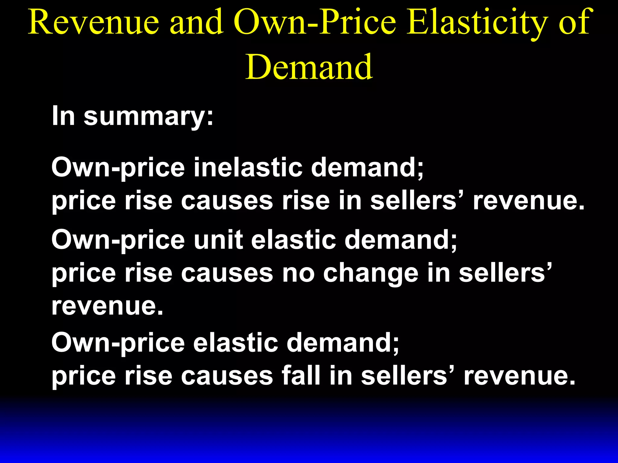
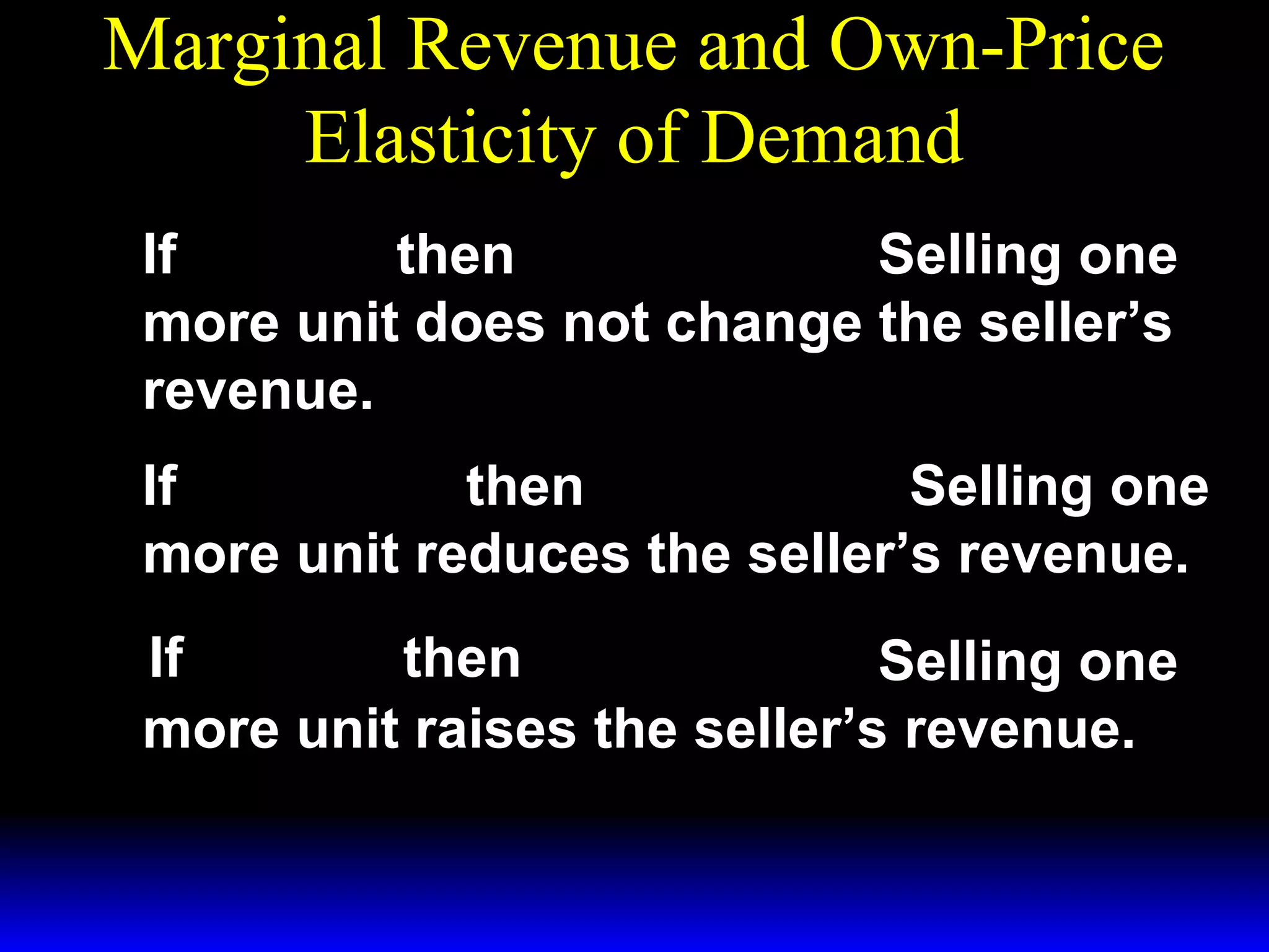
so if ε = −1
then
dR
=0
dp
and a change to price does not alter
sellers’ revenue.

55. Revenue and Own-Price Elasticity of
Demand
dR
= X* (p )[ 1 + ε ]
dp
dR
>0
but if − 1 < ε ≤ 0 then
dp
and a price increase raises sellers’
revenue.

56. Revenue and Own-Price Elasticity of
Demand
dR
= X* (p )[ 1 + ε ]
dp
And if
ε < −1
dR
<0
then
dp
and a price increase reduces sellers’
revenue.

57. Revenue and Own-Price Elasticity of
Demand
In summary:
Own-price inelastic demand; − 1 < ε ≤ 0
price rise causes rise in sellers’ revenue.
Own-price unit elastic demand; ε = −1
price rise causes no change in sellers’
revenue.
Own-price elastic demand; ε < −1
price rise causes fall in sellers’ revenue.

58. Marginal Revenue and Own-Price
Elasticity of Demand
A
seller’s marginal revenue is the rate
at which revenue changes with the
number of units sold by the seller.
dR( q)
MR( q) =
.
dq

59. Marginal Revenue and Own-Price
Elasticity of Demand
p(q) denotes the seller’s inverse demand
function; i.e. the price at which the seller
can sell q units. Then
R ( q) = p( q) × q
so
dR( q) dp( q)
MR( q) =
=
q + p( q)
dq
dq
q dp( q) 

= p( q) 1 +
.
 p( q) dq 

60. Marginal Revenue and Own-Price
Elasticity of Demand
q dp( q) 

MR( q) = p( q) 1 +
.
 p( q) dq 
and
so
dq p
ε=
×
dp q
1 + 1  .
MR( q) = p( q) 
ε



61. Marginal Revenue and Own-Price
Elasticity of Demand
1 + 1 
MR( q) = p( q) 
ε


says that the rate
at which a seller’s revenue changes
with the number of units it sells
depends on the sensitivity of quantity
demanded to price; i.e., upon the
of the own-price elasticity of demand.

62. Marginal Revenue and Own-Price
Elasticity of Demand
1 + 1
MR(q) = p(q)
 ε

If ε = −1
then MR( q) = 0.
If − 1 < ε ≤ 0 then MR( q) < 0.
If ε < −1
then MR( q) > 0.

63. Marginal Revenue and Own-Price
Elasticity of Demand
If ε = −1 then MR( q) = 0. Selling one
more unit does not change the seller’s
revenue.
If − 1 < ε ≤ 0 then MR( q) < 0. Selling one
more unit reduces the seller’s revenue.
If ε < −1 then MR( q) > 0. Selling one
more unit raises the seller’s revenue.

64. Marginal Revenue and Own-Price
Elasticity of Demand
An example with linear inverse demand.
p( q) = a − bq.
Then R( q) = p( q)q = ( a − bq)q
and
MR( q) = a − 2bq.

65. Marginal Revenue and Own-Price
Elasticity of Demand
p
a
p( q) = a − bq
a/2b
a/b
q
MR( q) = a − 2bq

66. Marginal Revenue and Own-Price
p
Elasticity of Demand
a
MR( q) = a − 2bq
p( q) = a − bq
$
a/2b
a/b
q
a/b
q
R(q)
a/2b