Ch 04.ppt

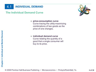
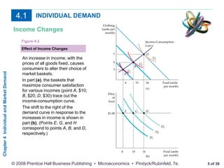
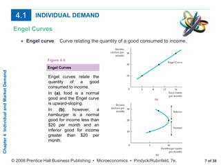
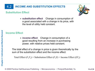
2 of 35
© 2008 Prentice Hall Business Publishing • Microeconomics • Robert S. Pindyck, 8e.
Chapter 4
Individual and Market Demand

Chapter
4
Individual
and
Market
Demand
2 of 38
© 2008 Prentice Hall Business Publishing • Microeconomics • Pindyck/Rubinfeld, 7e.
CHAPTER 4 OUTLINE
4.1 Individual Demand
4.2 Income and Substitution Effects
4.3 Market Demand
4.4 Consumer Surplus

Chapter
4
Individual
and
Market
Demand
3 of 38
INDIVIDUAL DEMAND
4.1
Price Changes
Effect of Price Changes
A reduction in the price of food,
with income and the price of
clothing fixed, causes this
consumer to choose a different
market basket.
In (a), the baskets that
maximize utility for various
prices of food (point A, $2; B,
$1; D, $0.50) trace out the
price-consumption curve.
Part (b) gives the demand
curve, which relates the price of
food to the quantity demanded.
(Points E, G, and H correspond
to points A, B, and D,
respectively).
Figure 4.1

Chapter
4
Individual
and
Market
Demand
4 of 38
INDIVIDUAL DEMAND
4.1
The Individual Demand Curve
● price-consumption curve
Curve tracing the utility-maximizing
combinations of two goods as the
price of one changes.
● individual demand curve
Curve relating the quantity of a
good that a single consumer will
buy to its price.

Chapter
4
Individual
and
Market
Demand
5 of 38
INDIVIDUAL DEMAND
4.1
Income Changes
Effect of Income Changes
An increase in income, with the
prices of all goods fixed, causes
consumers to alter their choice of
market baskets.
In part (a), the baskets that
maximize consumer satisfaction
for various incomes (point A, $10;
B, $20; D, $30) trace out the
income-consumption curve.
The shift to the right of the
demand curve in response to the
increases in income is shown in
part (b). (Points E, G, and H
correspond to points A, B, and D,
respectively.)
Figure 4.2

Chapter
4
Individual
and
Market
Demand
6 of 38
INDIVIDUAL DEMAND
4.1
Normal versus Inferior Goods
An Inferior Good
An increase in a person’s
income can lead to less
consumption of one of the
two goods being
purchased.
Here, hamburger, though
a normal good between A
and B, becomes an
inferior good when the
income-consumption
curve bends backward
between B and C.
Figure 4.3

Chapter
4
Individual
and
Market
Demand
7 of 38
INDIVIDUAL DEMAND
4.1
Engel Curves
Engel Curves
Engel curves relate the
quantity of a good
consumed to income.
In (a), food is a normal
good and the Engel curve
is upward-sloping.
In (b), however, a
hamburger is a normal
good for income less than
$20 per month and an
inferior good for income
greater than $20 per
month.
Figure 4.4
● Engel curve Curve relating the quantity of a good consumed to income.

Chapter
4
Individual
and
Market
Demand
8 of 38
INDIVIDUAL DEMAND
4.1
If the market price were held constant,
we would expect to see an increase in
the quantity demanded as a result of
consumers’ higher incomes. Because
this increase would occur no matter
what the market price, the result
would be a shift to the right of the
entire demand curve.

Chapter
4
Individual
and
Market
Demand
9 of 38
INDIVIDUAL DEMAND
4.1
TABLE 4.1 Annual U.S. Household Consumer Expenditures
INCOME GROUP (2005$)
Expenditures Less than 10,000- 20,000- 30,000- 40,000- 50,000 70,000
($) on: $10,000 19,999 29,999 39,999 49,999 69,999 and above
Entertainment 844 947 1191 1677 1933 2402 4542
Owned Dwelling 4272 4716 5701 6776 7771 8972 14763
Rented Dwelling 2672 2779 2980 2977 2818 2255 1379
Heath Care 1108 1874 2241 2361 2778 2746 3812
Food 2901 3242 3942 4552 5234 6570 9247
Clothing 861 884 1106 1472 1450 1961 3245
Source: U.S. Department of Labor, Bureau of Labor Statistics, “Consumer Expenditure Survey, Annual Report 2005.”

Chapter
4
Individual
and
Market
Demand
10 of 38
INDIVIDUAL DEMAND
4.1
Engel Curves for U.S.
Consumers
Average per-household
expenditures on rented
dwellings, health care,
and entertainment are
plotted as functions of
annual income.
Health care and
entertainment are normal
goods, as expenditures
increase with income.
Rental housing, however,
is an inferior good for
incomes above $35,000.
Figure 4.5

Chapter
4
Individual
and
Market
Demand
11 of 38
INDIVIDUAL DEMAND
4.1
Substitutes and Complements
Recall that:
Two goods are substitutes if an increase in the price of one
leads to an increase in the quantity demanded of the other.
Two goods are complements if an increase in the price of one
good leads to a decrease in the quantity demanded of the
other.
Two goods are independent if a change in the price of one
good has no effect on the quantity demanded of the other.

Chapter
4
Individual
and
Market
Demand
12 of 38
INCOME AND SUBSTITUTION EFFECTS
4.2
A fall in the price of a good has two effects:
1. Consumers will tend to buy more of the good that has
become cheaper and less of those goods that are now
relatively more expensive.
2. Because one of the goods is now cheaper, consumers
enjoy an increase in real purchasing power.

Chapter
4
Individual
and
Market
Demand
13 of 38
4.2
Income and Substitution Effects:
Normal Good
A decrease in the price of food
has both an income effect and a
substitution effect.
The consumer is initially at A, on
budget line RS.
When the price of food falls,
consumption increases by F1F2 as
the consumer moves to B.
The substitution effect F1E
(associated with a move from A to
D) changes the relative prices of
food and clothing but keeps real
income (satisfaction) constant.
The income effect EF2
(associated with a move from D to
B) keeps relative prices constant
but increases purchasing power.
Food is a normal good because
the income effect EF2 is positive.
Figure 4.6

Chapter
4
Individual
and
Market
Demand
14 of 38
4.2
Substitution Effect
● substitution effect Change in consumption of
a good associated with a change in its price, with
the level of utility held constant.
Income Effect
● income effect Change in consumption of a
good resulting from an increase in purchasing
power, with relative prices held constant.
Total Effect (F1F2) = Substitution Effect (F1E) + Income Effect (EF2)
The total effect of a change in price is given theoretically by the
sum of the substitution effect and the income effect:

Chapter
4
Individual
and
Market
Demand
15 of 38
4.2
Income and Substitution Effects:
Inferior Good
The consumer is initially at A on
budget line RS.
With a decrease in the price of food,
the consumer moves to B.
The resulting change in food
purchased can be broken down into a
substitution effect, F1E (associated
with a move from A to D), and an
income effect, EF2 (associated with a
move from D to B).
In this case, food is an inferior good
because the income effect is negative.
However, because the substitution
effect exceeds the income effect, the
decrease in the price of food leads to
an increase in the quantity of food
demanded.
Figure 4.7
Income Effect

Chapter
4
Individual
and
Market
Demand
16 of 38
4.2
Upward-Sloping Demand Curve: The
Giffen Good
When food is an inferior good, and
when the income effect is large
enough to dominate the
substitution effect, the demand
curve will be upward-sloping.
The consumer is initially at point
A, but, after the price of food falls,
moves to B and consumes less
food.
Because the income effect EF2 is
larger than the substitution effect
F1E, the decrease in the price of
food leads to a lower quantity of
food demanded.
Figure 4.8
A Special Case: The Giffen Good
● Giffen good Good whose demand curve slopes upward
because the (negative) income effect is larger than the
substitution effect.

Chapter
4
Individual
and
Market
Demand
17 of 38
4.2
Effect of a Gasoline Tax with a Rebate
Figure 4.9
A gasoline tax is imposed when
the consumer is initially buying
1200 gallons of gasoline at point
C.
After the tax takes effect, the
budget line shifts from AB to AD
and the consumer maximizes his
preferences by choosing E, with a
gasoline consumption of 900
gallons.
However, when the proceeds of
the tax are rebated to the
consumer, his consumption
increases somewhat, to 913.5
gallons at H.
Despite the rebate program, the
consumer’s gasoline consumption
has fallen, as has his level of
satisfaction.

Chapter
4
Individual
and
Market
Demand
18 of 38
MARKET DEMAND
4.3
● market demand curve Curve relating
the quantity of a good that all consumers
in a market will buy to its price.
From Individual to Market Demand
TABLE 4.2 Determining the Market Demand Curve
(1) (2) (3) (4) (5)
Price Individual A Individual B Individual C Market
($) (Units) (Units) (Units) (Units)
1 6 10 16 32
2 4 8 13 25
3 2 6 10 18
4 0 4 7 11
5 0 2 4 6

Chapter
4
Individual
and
Market
Demand
19 of 38
MARKET DEMAND
4.3
Summing to Obtain a Market Demand
Curve
The market demand curve is
obtained by summing our three
consumers’ demand curves DA,
DB, and DC.
At each price, the quantity of
coffee demanded by the market is
the sum of the quantities
demanded by each consumer.
At a price of $4, for example, the
quantity demanded by the market
(11 units) is the sum of the
quantity demanded by A (no
units), B (4 units), and C (7 units).
Figure 4.10

Chapter
4
Individual
and
Market
Demand
20 of 38
MARKET DEMAND
4.3
The aggregation of individual demands into market becomes
important in practice when market demands are built up from the
demands of different demographic groups or from consumers located
in different areas.
For example, we might obtain information about the demand for
home computers by adding independently obtained information about
the demands of the following groups:
• Households with children
• Households without children
• Single individuals
Two points should be noted:
1. The market demand curve will shift to the right as more
consumers enter the market.
2. Factors that influence the demands of many consumers will also
affect market demand.

Chapter
4
Individual
and
Market
Demand
21 of 38
MARKET DEMAND
4.3
Elasticity of Demand
Denoting the quantity of a good by Q and its price by P, the price
elasticity of demand is
(4.1)
Inelastic Demand
When demand is inelastic, the quantity demanded is relatively
unresponsive to changes in price. As a result, total expenditure on the
product increases when the price increases.
Elastic Demand
When demand is elastic, total expenditure on the product decreases
as the price goes up.

Chapter
4
Individual
and
Market
Demand
22 of 38
MARKET DEMAND
4.3
Isoelastic Demand
● isoelastic demand curve Demand curve with a constant price
elasticity.
Unit-Elastic Demand Curve
When the price elasticity
of demand is −1.0 at
every price, the total
expenditure is constant
along the demand curve
D.
Figure 4.11

Chapter
4
Individual
and
Market
Demand
23 of 38
MARKET DEMAND
4.3
Isoelastic Demand
TABLE 4.3 Price Elasticity and Consumer Expenditures
Demand If Price Increases, If Price Decreases,
Expenditures Expenditures
Inelastic Increase Decrease
Unit elastic Are unchanged Are unchanged
Elastic Decrease Increase

Chapter
4
Individual
and
Market
Demand
24 of 38
4.3
Domestic demand for wheat is given by the equation
QDD = 1430 – 55P
where QDD is the number of bushels (in millions) demanded
domestically, and P is the price in dollars per bushel. Export demand
is given by
QDE = 1470 − 70P
where QDE is the number of bushels (in millions) demanded from
abroad.
To obtain the world demand for wheat, we set the left side of each
demand equation equal to the quantity of wheat. We
then add the right side of the equations, obtaining
QDD + QDE = (1430 − 55P) + (1470 − 70P) = 2900 − 125P
MARKET DEMAND

Chapter
4
Individual
and
Market
Demand
25 of 38
4.3 MARKET DEMAND
The Aggregate Demand for
Wheat
The total world demand
for wheat is the
horizontal sum of the
domestic demand AB
and the export demand
CD.
Even though each
individual demand curve
is linear, the market
demand curve is kinked,
reflecting the fact that
there is no export
demand when the price
of wheat is greater than
about $21 per bushel.
Figure 4.12

Chapter
4
Individual
and
Market
Demand
26 of 38
4.3 MARKET DEMAND
TABLE 4.4 Price and Income Elasticities of the Demand of Rooms
Group Price Elasticity Income Elasticity
Single individuals −0.10 0.21
Married, head of household −0.25 0.06
age less than 30, 1 child
Married, head age 30–39, −0.15 0.12
2 or more children
Married, head age 50 or −0.08 0.19
older, 1 child

Chapter
4
Individual
and
Market
Demand
27 of 38
4.4 CONSUMER SURPLUS
● consumer surplus Difference between what a consumer is willing to
pay for a good and the amount actually paid.
Consumer Surplus and Demand
Consumer Surplus
Consumer surplus is the
total benefit from the
consumption of a product,
less the total cost of
purchasing it.
Here, the consumer surplus
associated with six concert
tickets (purchased at $14
per ticket) is given by the
yellow-shaded area.
Figure 14.3

Chapter
4
Individual
and
Market
Demand
28 of 38
Consumer Surplus Generalized
For the market as a whole, consumer
surplus is measured by the area
under the demand curve and above
the line representing the purchase
price of the good.
Here, the consumer surplus is given
by the yellow-shaded triangle and is
equal to
1/2 × ($20 − $14) × 6500 = $19,500.
Figure 14.4
When added over many individuals, it measures the aggregate benefit that
consumers obtain from buying goods in a market.
When we combine consumer surplus with the aggregate profits that producers
obtain, we can evaluate both the costs and benefits of alternative market
structures and public policies.

Chapter
4
Individual
and
Market
Demand
29 of 38
To encourage cleaner air, Congress passed the
Clean Air Act in 1977 and has since amended it a
number of times.
Valuing Cleaner Air
Figure 14.5
The yellow-shaded triangle gives
the consumer surplus generated
when air pollution is reduced by 5
parts per 100 million of nitrogen
oxide at a cost of $1000 per part
reduced.
The surplus is created because
most consumers are willing to pay
more than $1000 for each unit
reduction of nitrogen oxide.

Ch 04.ppt

More Related Content

What's hot

Similar to Ch 04.ppt

Recently uploaded

Ch 04.ppt

Editor's Notes