Syllabus
1 Introduction toData Structure: Fundamentals of Data Structure, Operations of Data Structure: Traversing, Inserting and Deleting, Arrays as Data Structure,
Searching, Sorting Bubble, Insertion, Selection).
2 Stacks: Introduction and Definition, Representation, Operations on Stacks,
Applications of Stacks, Representation of Arithmetic Expressions: Infix, Postfix, Prefix.
3 Queues: Introduction and Definition, Representation, Operation on Queues, Types of Queues, Dequeue, Circular Queue, Priority Queue, Applications of
Queue.
4 Linked List: Definition of Linked List, Dynamic Memory Management,
Representation of Linked List, Operations on Linked List, Inserting, Removing, Searching, Sorting, Merging Nodes , Double Linked List
5 Trees : Definition of Tree, Binary Tree and their types, Representation of Binary Tree, Operations on Binary Tree, Binary Search Tree (BST), Traversal of Binary
Tree, Preorder Traversal, In-order Traversal, Post-order Traversal,
Introduction of Threaded Binary Tree, AVL Tree and B-Tree.
6 Graphs: Definition of Graph, Basic Concepts of Graph, Representation of Graph, Adjacency Matrix, Adjacency List, Graph Traversal:
Breadth First Search (BFS), Depth First Search (DFS)
3.
Reference Books
• DataStructures Using C 2E: Reema Thareja, Oxford Higher Education
• Data Structures Using C and C++ : Yedidyah Langsam, Moshe Augenstein,
Aaron Tenenbaum, PHI,2nd Ed.
• Magnifying Data Structures : Arpita Gopal, PHI Learning Pvt. Ltd
• The Ultimate C with Data Structures: R. Nageswara Rao, Dreamtech
publications
• Data Structure through C Y.P. Kanetkar, BPB,2nd Ed.
• Data Structures with C: Schaums Outlines Hubbard John
• Data Structures Using C and C++ (Tenenbaum) Tenenbaum, Pearson Pub.
• Fundamental of Data Structure in C Horowitz Sahani, Galgotia pub.
4.
• Introduction toData Structure
• Fundamentals of Data Structure
• Operations of Data Structure: Traversing, Inserting and Deleting
Arrays as Data Structure
• Searching
• Sorting Bubble, Insertion, Selection
5.
Understanding Data Structures
•Imagine you are the librarian of a large public library with
over 10,000 books.
• Your task is to organize these books efficiently.
• How would you organize this library so that you can quickly
find, add, remove, and categorize books?
6.
Understanding Data Structures
Formsmall groups for this activity. Each group will be assigned a different library task,
• Group 1: Managing a book return counter .
• Group 2: Organizing a checkout line.
• Group 3: Creating a digital catalog .
• Group 4: Recommending similar books based on connections.
Each group has to discuss and present how their assigned structure helps in managing the library efficiently.
7.
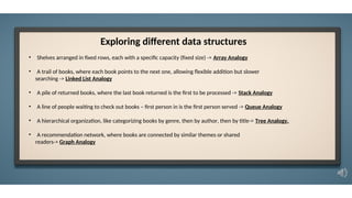
• Shelves arrangedin fixed rows, each with a specific capacity (fixed size) -> Array Analogy
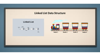
• A trail of books, where each book points to the next one, allowing flexible addition but slower
searching -> Linked List Analogy
• A pile of returned books, where the last book returned is the first to be processed -> Stack Analogy
• A line of people waiting to check out books – first person in is the first person served -> Queue Analogy
• A hierarchical organization, like categorizing books by genre, then by author, then by title-> Tree Analogy.
• A recommendation network, where books are connected by similar themes or shared
readers-> Graph Analogy
Exploring different data structures
8.
• Efficient DataManagement: Organizes data for quick access and modification.
• Optimized Performance: Reduces time complexity for operations like searching,
sorting, and traversal.
• Memory Efficiency: Minimizes the memory footprint by storing only what is necessary.
• Data Integrity: Maintains relationships between data elements effectively.
• Scalability: Handles large volumes of data without significant performance loss.
Why use Data Structures?
9.
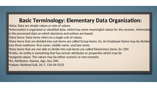
Basic Terminology: ElementaryData Organization:
•Data: Data are simply values or sets of values.
•Information is organized or classified data, which has some meaningful values for the receiver. Information
is the processed data on which decisions and actions are based.
•Data items: Data items refers to a single unit of values.
•Data items that are divided into sub-items are called Group items. Ex: An Employee Name may be divided
into three subitems- first name, middle name, and last name.
•Data items that are not able to divide into sub-items are called Elementary items. Ex: SSN
•Entity: An entity is something that has certain attributes or properties which may be
•assigned values. The values may be either numeric or non-numeric.
•Ex: Attributes- Names, Age, Sex, SSN
•Values- Rohland Gail, 34, F, 134-34-5533
11.
Arrays:
The simplest typeof data structure is a linear (or one dimensional) array. A list of a finite number n of similar
data referenced respectively by a set of n consecutive numbers, usually 1, 2, 3 . . . . . . . n. if A is chosen the name
for the array, then the elements of A are denoted by subscript notation a1, a2, a3..... an
by the bracket notation A [1], A [2], A [3] . . . . . . A [n]
12.
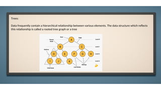
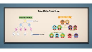
Trees:
Data frequently containa hierarchical relationship between various elements. The data structure which reflects
this relationship is called a rooted tree graph or a tree
13.
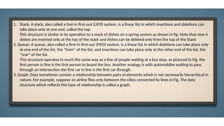
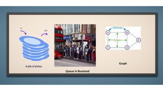
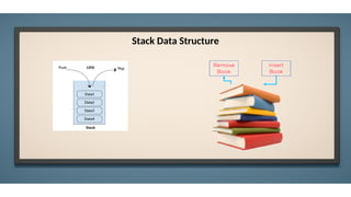
1. Stack: Astack, also called a fast-in first-out (LIFO) system, is a linear list in which insertions and deletions can
take place only at one end, called the top.
This structure is similar in its operation to a stack of dishes on a spring system as shown in fig. Note that new 4
dishes are inserted only at the top of the stack and dishes can be deleted only from the top of the Stack
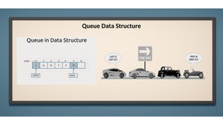
2. Queue: A queue, also called a first-in first-out (FIFO) system, is a linear list in which deletions can take place only
at one end of the list, the "from'' of the list, and insertions can take place only at the other end of the list, the
“rear” of the list.
This structure operates in much the same way as a line of people waiting at a bus stop, as pictured in Fig. the
first person in line is the first person to board the bus. Another analogy is with automobiles waiting to pass
through an intersection the first car in line is the first car through.
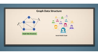
3. Graph: Data sometimes contain a relationship between pairs of elements which is not necessarily hierarchical in
nature. For example, suppose an airline flies only between the cities connected by lines in Fig. The data
structure which reflects this type of relationship is called a graph.
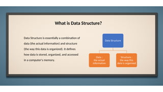
What is DataStructure?
Data Structure is essentially a combination of
data (the actual information) and structure
(the way this data is organized). It defines
how data is stored, organized, and accessed
in a computer's memory.
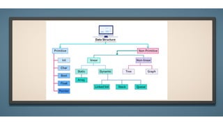
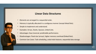
Linear Data Structures
•Elements are arranged in a sequential order.
• Memory is typically allocated in a contiguous manner (except linked lists).
• Simple to implement and understand.
• Examples: Arrays, Stacks, Queues, Linked Lists.
• Advantages: Easy traversal, predictable performance.
• Disadvantages: Fixed size (arrays), higher memory overhead (linked lists).
• Common Use Cases: Task scheduling, undo/redo features, sequential data storage.
18.
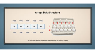
Arrays Data Structure
AnArray is a collection of elements, each identified by an index or a key.
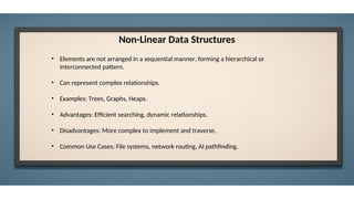
Non-Linear Data Structures
•Elements are not arranged in a sequential manner, forming a hierarchical or
interconnected pattern.
• Can represent complex relationships.
• Examples: Trees, Graphs, Heaps.
• Advantages: Efficient searching, dynamic relationships.
• Disadvantages: More complex to implement and traverse.
• Common Use Cases: File systems, network routing, AI pathfinding.
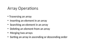
Array Operations
• Traversingan array
• Inserting an element in an array
• Searching an element in an array
• Deleting an element from an array
• Merging two arrays
• Sorting an array in ascending or descending order
26.
Traversing an array
#include<stdio.h>
#include <conio.h>
int main()
{
int i, n, arr[20];
clrscr();
printf("n Enter the number of elements in the array : ");
scanf("%d", &n);
for(i=0;i<n;i++)
{
printf("n arr[%d] = ", i);
scanf("%d",&arr[i]);
}
printf("n The array elements are ");
for(i=0;i<n;i++)
printf("t %d", arr[i]);
return 0;
}
27.
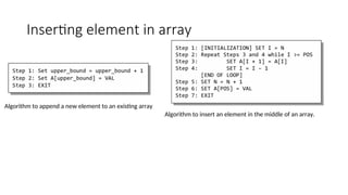
Inserting element inarray
Algorithm to append a new element to an existing array
Algorithm to insert an element in the middle of an array.
28.
int main()
{
int i,n, num, pos, arr[10];
clrscr();
printf("n Enter the number of
elements in the array : ");
scanf("%d", &n);
for(i=0;i<n;i++)
{
printf("n arr[%d] = ", i);
scanf("%d", &arr[i]);
}
printf("n Enter the number to be inserted : ");
scanf("%d", &num);
printf("n Enter the position at which the
number has to be added : ");
scanf("%d", &pos);
for(i=n–1;i>=pos;i––)
arr[i+1] = arr[i];
arr[pos] = num;
n = n+1;
printf("n The array after insertion of %d is : ",
num);
for(i=0;i<n;i++)
printf("n arr[%d] = %d", i, arr[i]);
getch();
return 0;
}
29.
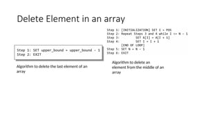
Delete Element inan array
Algorithm to delete the last element of an
array
Algorithm to delete an
element from the middle of an
array
30.
int main()
{
}
Output
int i,n, pos, arr[10];
clrscr();
printf("n Enter the number of elements in the array : ");
scanf("%d", &n);
for(i=0;i<n;i++)
{
printf("n arr[%d] = ", i);
scanf("%d", &arr[i]);
}
printf("nEnter the position from which the number
has to be deleted : ");
scanf("%d", &pos);
for(i=pos; i<n–1;i++)
arr[i] = arr[i+1];
n– –;
printf("n The array after deletion is : ");
for(i=0;i<n;i++)
printf("n arr[%d] = %d", i, arr[i]);
getch();
return 0;
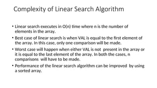
Complexity of LinearSearch Algorithm
• Linear search executes in O(n) time where n is the number of
elements in the array.
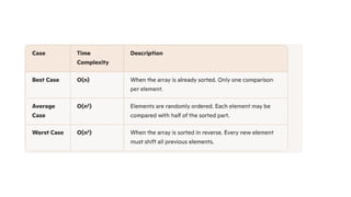
• Best case of linear search is when VAL is equal to the first element of
the array. In this case, only one comparison will be made.
• Worst case will happen when either VAL is not present in the array or
it is equal to the last element of the array. In both the cases, n
comparisons will have to be made.
• Performance of the linear search algorithm can be improved by using
a sorted array.
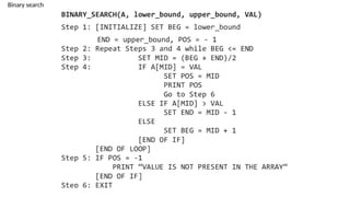
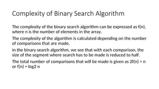
Complexity of BinarySearch Algorithm
The complexity of the binary search algorithm can be expressed as f(n),
where n is the number of elements in the array.
The complexity of the algorithm is calculated depending on the number
of comparisons that are made.
In the binary search algorithm, we see that with each comparison, the
size of the segment where search has to be made is reduced to half.
The total number of comparisons that will be made is given as 2f(n) > n
or f(n) = log2 n
35.
#include <stdio.h>
int main(){
int A[100], n, x, i = 1, found = 0;
printf("Enter number of elements (n):
");
scanf("%d", &n);
printf("Enter %d elements:n", n);
for (int j = 0; j < n; j++) {
scanf("%d", &A[j]);
}
printf("Enter value to search (x): ");
scanf("%d", &x);
while (i <= n) {
if (A[i - 1] == x) {
printf("Element %d found
at index %dn", x, i);
found = 1;
break;
}
i++;
}
if (!found) {
printf("Element %d not
foundn", x);
}
return 0;
}
36.
Sorting
BUBBLE_SORT(A, N)
Step 1:Repeat Step2 For I= 0to N-1
Step 2:
Repeat For J=0 to N-I
Step 3:
IF A[J]>A[J + 1]
SWAP A[J] and A[J+1]
[END OF INNER LOOP]
[END OF OUTER LOOP]
Step 4: EXIT
37.
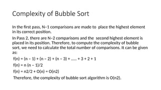
Complexity of BubbleSort
In the first pass, N–1 comparisons are made to place the highest element
in its correct position.
In Pass 2, there are N–2 comparisons and the second highest element is
placed in its position. Therefore, to compute the complexity of bubble
sort, we need to calculate the total number of comparisons. It can be given
as:
f(n) = (n – 1) + (n – 2) + (n – 3) + ..... + 3 + 2 + 1
f(n) = n (n – 1)/2
f(n) = n2/2 + O(n) = O(n2)
Therefore, the complexity of bubble sort algorithm is O(n2).
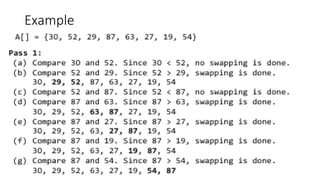
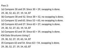
Pass 2:
(a) Compare30 and 29. Since 30 > 29, swapping is done.
29, 30, 52, 63, 27, 19, 54, 87
(b) Compare 30 and 52. Since 30 < 52, no swapping is done.
(c) Compare 52 and 63. Since 52 < 63, no swapping is done.
(d) Compare 63 and 27. Since 63 > 27, swapping is done.
29, 30, 52, 27, 63, 19, 54, 87
(e) Compare 63 and 19. Since 63 > 19, swapping is done.
436 Data Structures Using C
29, 30, 52, 27, 19, 63, 54, 87
(f) Compare 63 and 54. Since 63 > 54, swapping is done.
29, 30, 52, 27, 19, 54, 63, 87
40.
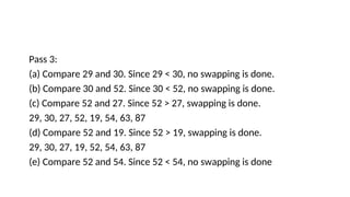
Pass 3:
(a) Compare29 and 30. Since 29 < 30, no swapping is done.
(b) Compare 30 and 52. Since 30 < 52, no swapping is done.
(c) Compare 52 and 27. Since 52 > 27, swapping is done.
29, 30, 27, 52, 19, 54, 63, 87
(d) Compare 52 and 19. Since 52 > 19, swapping is done.
29, 30, 27, 19, 52, 54, 63, 87
(e) Compare 52 and 54. Since 52 < 54, no swapping is done
41.
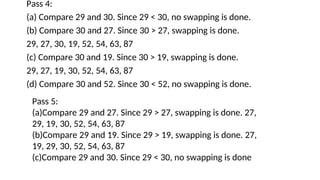
Pass 4:
(a) Compare29 and 30. Since 29 < 30, no swapping is done.
(b) Compare 30 and 27. Since 30 > 27, swapping is done.
29, 27, 30, 19, 52, 54, 63, 87
(c) Compare 30 and 19. Since 30 > 19, swapping is done.
29, 27, 19, 30, 52, 54, 63, 87
(d) Compare 30 and 52. Since 30 < 52, no swapping is done.
Pass 5:
(a)Compare 29 and 27. Since 29 > 27, swapping is done. 27,
29, 19, 30, 52, 54, 63, 87
(b)Compare 29 and 19. Since 29 > 19, swapping is done. 27,
19, 29, 30, 52, 54, 63, 87
(c)Compare 29 and 30. Since 29 < 30, no swapping is done
42.
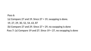
Pass 6:
(a) Compare27 and 19. Since 27 > 19, swapping is done.
19, 27, 29, 30, 52, 54, 63, 87
(b) Compare 27 and 29. Since 27 < 29, no swapping is done
Pass 7: (a) Compare 19 and 27. Since 19 < 27, no swapping is done
44.
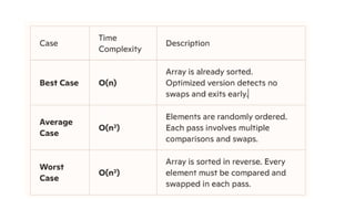
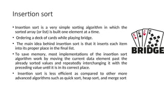
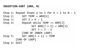
Insertion sort
• Insertionsort is a very simple sorting algorithm in which the
sorted array (or list) is built one element at a time.
• Ordering a deck of cards while playing bridge.
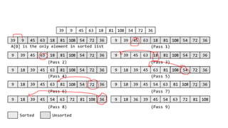
• The main idea behind insertion sort is that it inserts each item
into its proper place in the final list.
• To save memory, most implementations of the insertion sort
algorithm work by moving the current data element past the
already sorted values and repeatedly interchanging it with the
preceding value until it is in its correct place.
• Insertion sort is less efficient as compared to other more
advanced algorithms such as quick sort, heap sort, and merge sort
48.
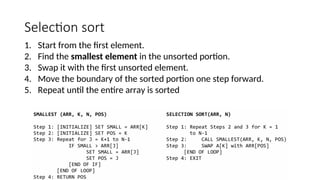
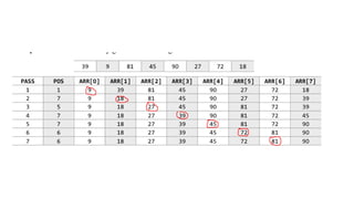
Selection sort
1. Startfrom the first element.
2. Find the smallest element in the unsorted portion.
3. Swap it with the first unsorted element.
4. Move the boundary of the sorted portion one step forward.
5. Repeat until the entire array is sorted
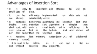
Advantages of InsertionSort
• It is easy to implement and efficient to use on
small sets of data.
• It can be efficiently implemented on data sets that
are already substantiallysorted.
• It performs betterthan algorithms like selection sort and
bubble sort. Insertion sort algorithm is simpler than
shell sort, with only a small trade off in efficiency. It is
over twice as fast as the bubble sort and almost 40
per cent faster than the selection sort.
• it requires less memory space (only O(1) of additional
memory space).
• it is said to be online, as it can sort a list as
and when it receives new elements.
53.
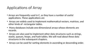
Applications of Array
•Arrays are frequently used in C, as they have a number of useful
applications. These applications are
• Arrays are widely used to implement mathematical vectors, matrices, and
other kinds of rectangular tables.
• Many databases include one-dimensional arrays whose elements are
records.
• Arrays are also used to implement other data structures such as strings,
stacks, queues, heaps, and hash tables. We will read about these data
structures in the subsequent chapters.
• Arrays can be used for sorting elements in ascending or descending order.
54.
#include <stdio.h>
int main(){
int arr[] = {7, 2, 9, 6, 4};
int length = sizeof(arr) / sizeof(arr[0]); // Calculate array length
printf("Array elements:n");
for (int i = 0; i < length; i++) {
printf("Element at index %d: %dn", i, arr[i]);
}
return 0;
}
Editor's Notes
#5 Activity: Data Structures
Imagine you are the librarian of a large public library with over 10,000 books. Your task is to organize these books efficiently.
How would you organize this library so that you can quickly find, add, remove, and categorize books?
Responses: Alphabetical order, by genre, by author, digital catalog, etc.
Expected Responses: Alphabetical order, by genre, by author, digital catalog, etc.
#6 Class Activity
Form small groups for this activity. Each group will be assigned a different library task,
Group 1: Managing a book return counter .
Group 2: Organizing a checkout line.
Group 3: Creating a digital catalog .
Group 4: Recommending similar books based on connections.
Each group has to discuss and present how their assigned data structure helps in managing the library efficiently.
#7 Let’s understand what different data structures can be used for Library Management
When managing a library, we need ways to store, access, and organize information efficiently. Data structures help us do just that! Let’s explore different types of data structures using real-life library examples:
Array – Shelves with Fixed Rows(You can easily access a book if you know its exact position (like the 3rd book on the 2nd shelf).
Linked List – A Trail of Books(Picture a trail of books, where each book has a note pointing to the next one.
You can keep adding books without worrying about shelf size)
Stack – A Pile of Returned Books(Books are stacked on top of each other.)
Queue – Line at the Checkout Counter
Imagine people waiting in line to check out books.
The first person in line is the first to be served.
Tree – Categorizing Books Hierarchically
Books are categorized by Genre → Author → Title.
This structure allows us to search quickly and stay organized.
Graph – Book Recommendation Network
Imagine a web where books are linked if they share a genre, theme, or are read by the same people.
#8 We use Data Structures because
It is efficient in Data Management- Organizes data for quick access and modification.
It optimize performance -Reduces time complexity for operations like searching, sorting, and traversal.
It manage Memory Efficiently: Minimizes the memory footprint by storing only what is necessary.
It uses data Integrity- Maintains relationships between data elements effectively.
It is Scalable - Handles large volumes of data without significant performance loss.
#15 Understanding the Components:
Data: The raw values or elements you want to store (e.g., numbers, characters, records).
Structure: The logical or physical arrangement of this data to make it usable and efficient for computation.
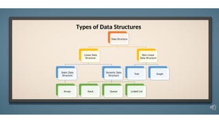
#16 The above diagram shows the types of data structures.
#17 Linear Data Structures were
Elements are arranged in a sequential order.
Memory is typically allocated in a contiguous manner (except linked lists).
Simple to implement and understand.
Examples: Arrays, Stacks, Queues, Linked Lists.
Advantages: Easy traversal, predictable performance.
Disadvantages: Fixed size (arrays), higher memory overhead (linked lists).
Common Use Cases: Task scheduling, undo/redo features, sequential data storage.
#18 An Array is a collection of elements, each identified by an index or a key. It is a fixed-size, sequential data structure that stores elements of the same data type in contiguous memory locations.
#19 A Stack is a linear data structure that follows the Last In, First Out (LIFO) principle, meaning the last element added is the first one to be removed. It works like a stack of plates, where you add and remove from the top.. It works like a stack of plates, where you add and remove from the top.
#20 A Queue is a linear data structure that follows the First In, First Out (FIFO) principle, meaning the first element added is the first one to be removed. It is like a real-world queue, such as a line of people waiting for a ticket, where the first person to join the line is the first to be served.
#21 Think of a linked list like a train, where each carriage is connected to the next by a coupling, forming a continuous chain that moves together as the train advances.
#22 Non-Linear Data Structure:
Elements are not stored sequentially – instead, they form hierarchies or networks.
Key Characteristics:
Represent complex relationships
Allow branching and interconnections
Examples:
Trees – for hierarchical data (e.g., file systems)
Graphs – for interconnected data (e.g., social networks, maps)
Advantages:
Efficient searching and decision-making
Ideal for representing dynamic or real-world relationships
Disadvantages:
More complex to build and navigate
Requires careful memory management
#23 A Tree is a hierarchical data structure that represents relationships in a branching format, similar to a family tree or an organizational chart. It consists of nodes connected by edges, with one node designated as the root.
#24 A Graph is a more generalized, non-linear data structure consisting of nodes (vertices) connected by edges. Unlike trees, graphs can have cycles and multiple paths between nodes.

![Arrays:
The simplest type of data structure is a linear (or one dimensional) array. A list of a finite number n of similar
data referenced respectively by a set of n consecutive numbers, usually 1, 2, 3 . . . . . . . n. if A is chosen the name
for the array, then the elements of A are denoted by subscript notation a1, a2, a3..... an
by the bracket notation A [1], A [2], A [3] . . . . . . A [n]](https://image.slidesharecdn.com/unit-1-251129064240-c726d9b0/85/C-programming-unit1-notes-syllabus-and-notes-11-320.jpg)
![Traversing an array
#include <stdio.h>
#include <conio.h>
int main()
{
int i, n, arr[20];
clrscr();
printf("n Enter the number of elements in the array : ");
scanf("%d", &n);
for(i=0;i<n;i++)
{
printf("n arr[%d] = ", i);
scanf("%d",&arr[i]);
}
printf("n The array elements are ");
for(i=0;i<n;i++)
printf("t %d", arr[i]);
return 0;
}](https://image.slidesharecdn.com/unit-1-251129064240-c726d9b0/85/C-programming-unit1-notes-syllabus-and-notes-26-320.jpg)
![int main()
{
int i, n, num, pos, arr[10];
clrscr();
printf("n Enter the number of
elements in the array : ");
scanf("%d", &n);
for(i=0;i<n;i++)
{
printf("n arr[%d] = ", i);
scanf("%d", &arr[i]);
}
printf("n Enter the number to be inserted : ");
scanf("%d", &num);
printf("n Enter the position at which the
number has to be added : ");
scanf("%d", &pos);
for(i=n–1;i>=pos;i––)
arr[i+1] = arr[i];
arr[pos] = num;
n = n+1;
printf("n The array after insertion of %d is : ",
num);
for(i=0;i<n;i++)
printf("n arr[%d] = %d", i, arr[i]);
getch();
return 0;
}](https://image.slidesharecdn.com/unit-1-251129064240-c726d9b0/85/C-programming-unit1-notes-syllabus-and-notes-28-320.jpg)
![int main()
{
}
Output
int i, n, pos, arr[10];
clrscr();
printf("n Enter the number of elements in the array : ");
scanf("%d", &n);
for(i=0;i<n;i++)
{
printf("n arr[%d] = ", i);
scanf("%d", &arr[i]);
}
printf("nEnter the position from which the number
has to be deleted : ");
scanf("%d", &pos);
for(i=pos; i<n–1;i++)
arr[i] = arr[i+1];
n– –;
printf("n The array after deletion is : ");
for(i=0;i<n;i++)
printf("n arr[%d] = %d", i, arr[i]);
getch();
return 0;](https://image.slidesharecdn.com/unit-1-251129064240-c726d9b0/85/C-programming-unit1-notes-syllabus-and-notes-30-320.jpg)
![#include <stdio.h>
int main() {
int A[100], n, x, i = 1, found = 0;
printf("Enter number of elements (n):
");
scanf("%d", &n);
printf("Enter %d elements:n", n);
for (int j = 0; j < n; j++) {
scanf("%d", &A[j]);
}
printf("Enter value to search (x): ");
scanf("%d", &x);
while (i <= n) {
if (A[i - 1] == x) {
printf("Element %d found
at index %dn", x, i);
found = 1;
break;
}
i++;
}
if (!found) {
printf("Element %d not
foundn", x);
}
return 0;
}](https://image.slidesharecdn.com/unit-1-251129064240-c726d9b0/85/C-programming-unit1-notes-syllabus-and-notes-35-320.jpg)
![Sorting
BUBBLE_SORT(A, N)
Step 1: Repeat Step2 For I= 0to N-1
Step 2:
Repeat For J=0 to N-I
Step 3:
IF A[J]>A[J + 1]
SWAP A[J] and A[J+1]
[END OF INNER LOOP]
[END OF OUTER LOOP]
Step 4: EXIT](https://image.slidesharecdn.com/unit-1-251129064240-c726d9b0/85/C-programming-unit1-notes-syllabus-and-notes-36-320.jpg)
![#include <stdio.h>
int main() {
int arr[] = {7, 2, 9, 6, 4};
int length = sizeof(arr) / sizeof(arr[0]); // Calculate array length
printf("Array elements:n");
for (int i = 0; i < length; i++) {
printf("Element at index %d: %dn", i, arr[i]);
}
return 0;
}](https://image.slidesharecdn.com/unit-1-251129064240-c726d9b0/85/C-programming-unit1-notes-syllabus-and-notes-54-320.jpg)


![DSA Ch1(Introduction) [Recovered].pptx](https://cdn.slidesharecdn.com/ss_thumbnails/dsach1introductionrecovered-240829154107-a96d835d-thumbnail.jpg?width=640&height=640&fit=bounds)