Downloaded 332 times

![Breadth First Search
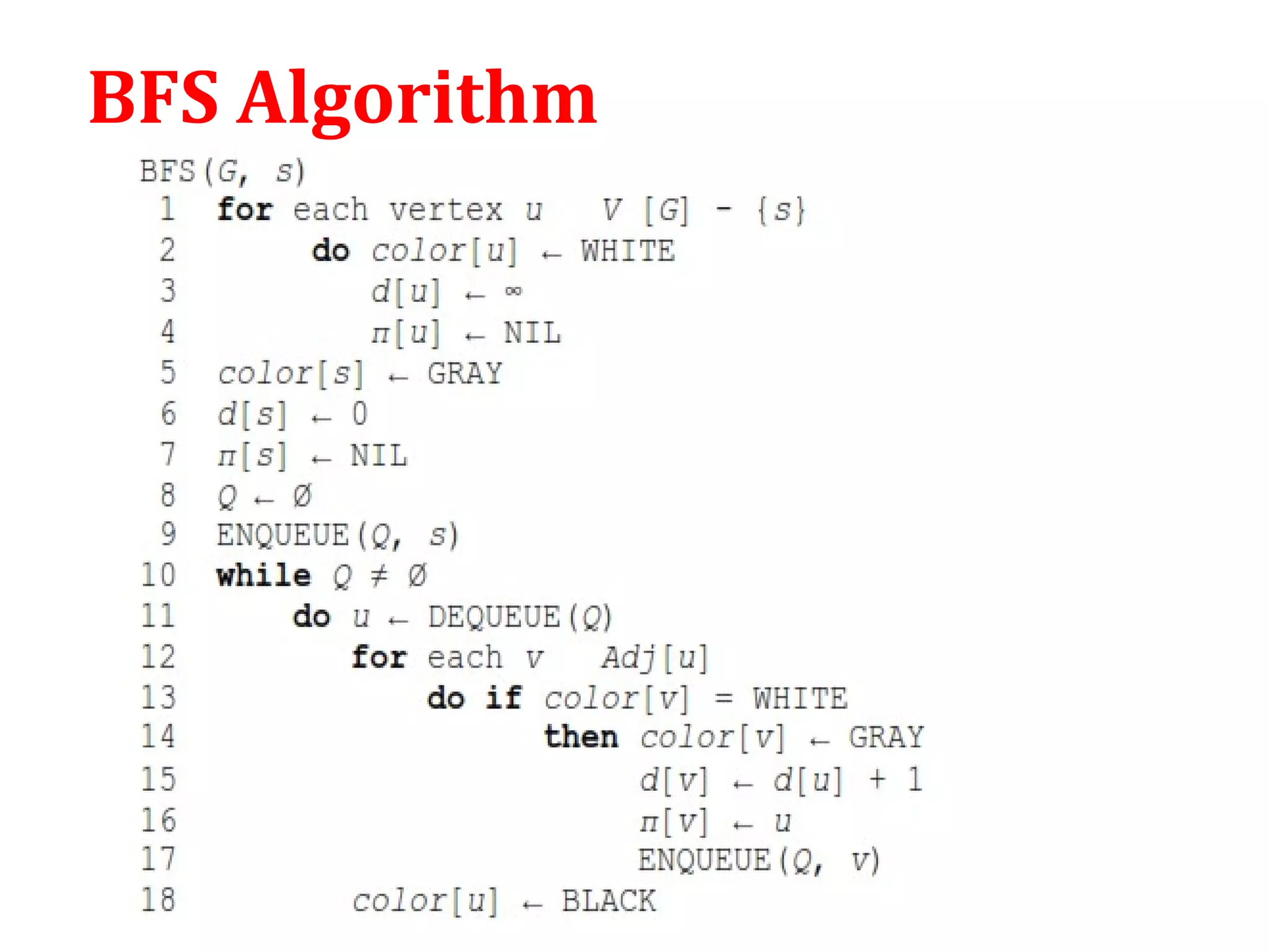
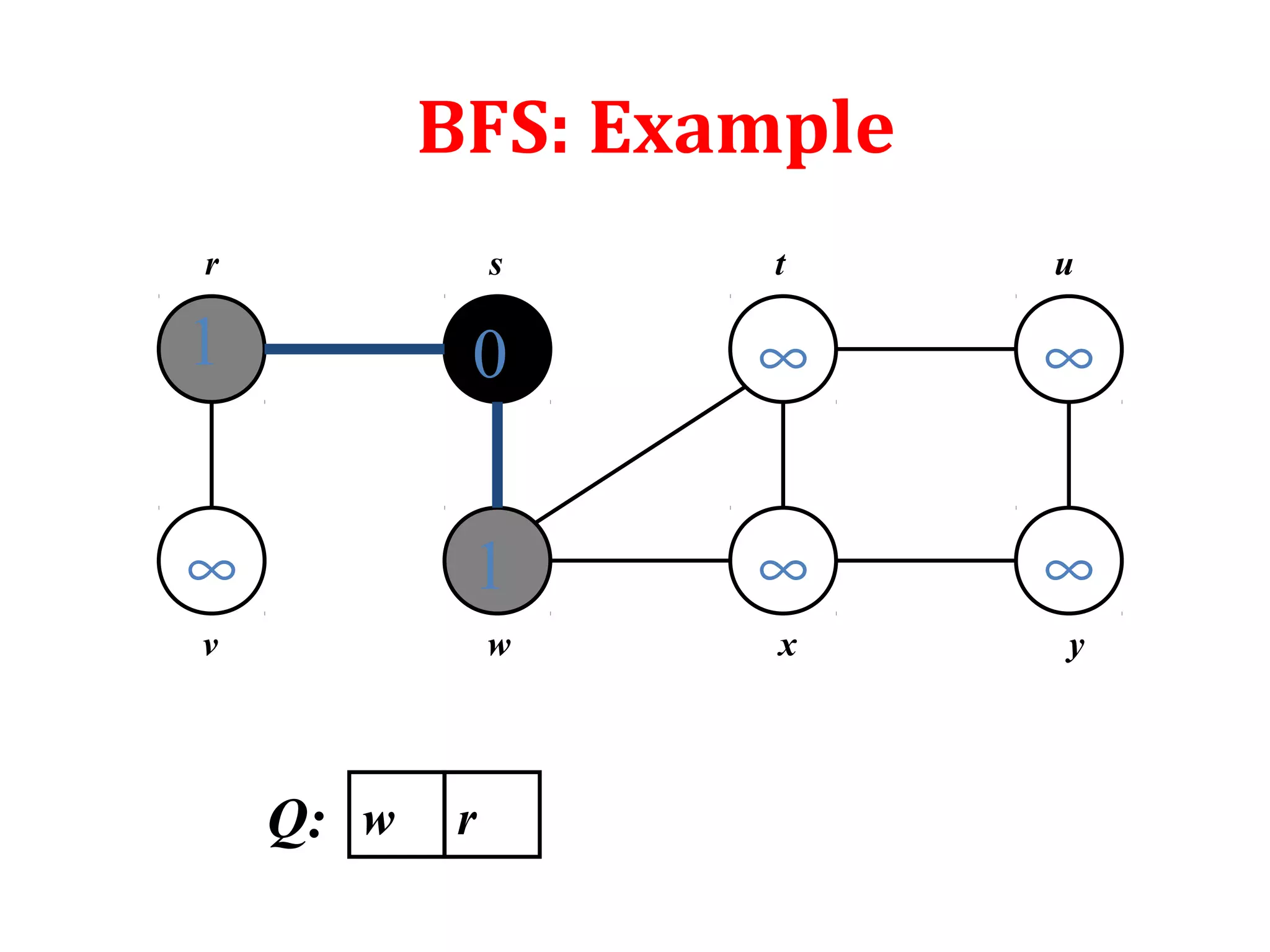
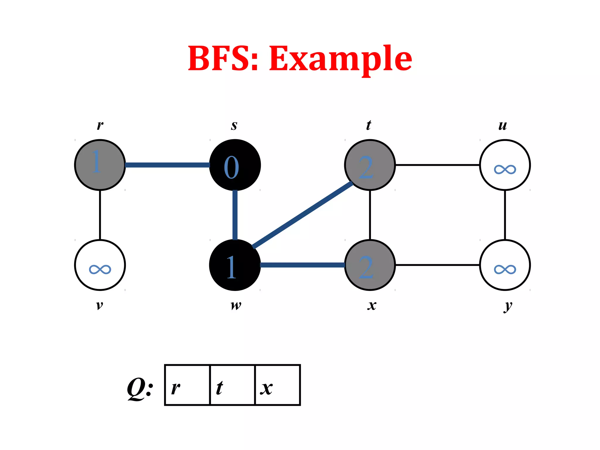
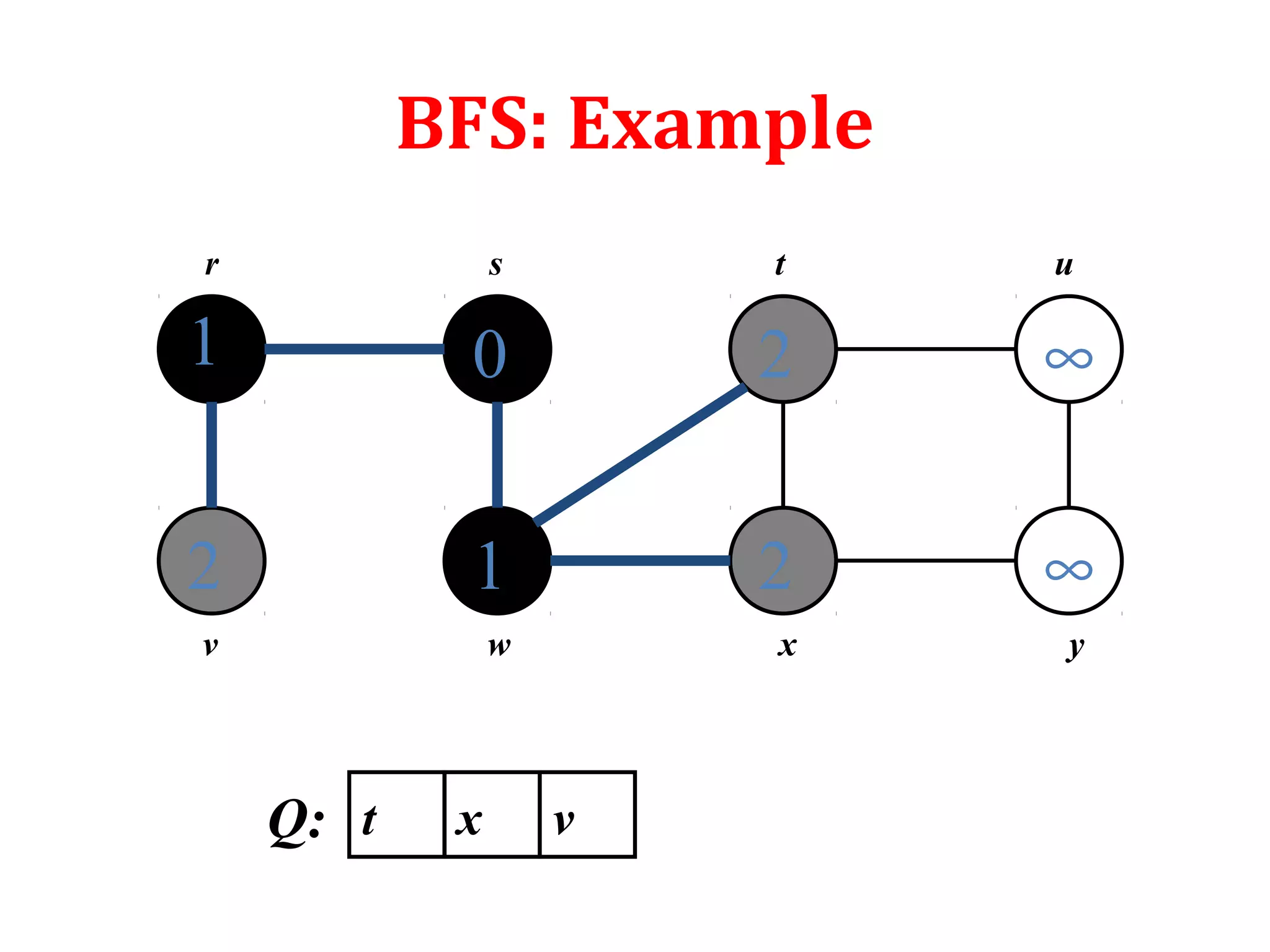
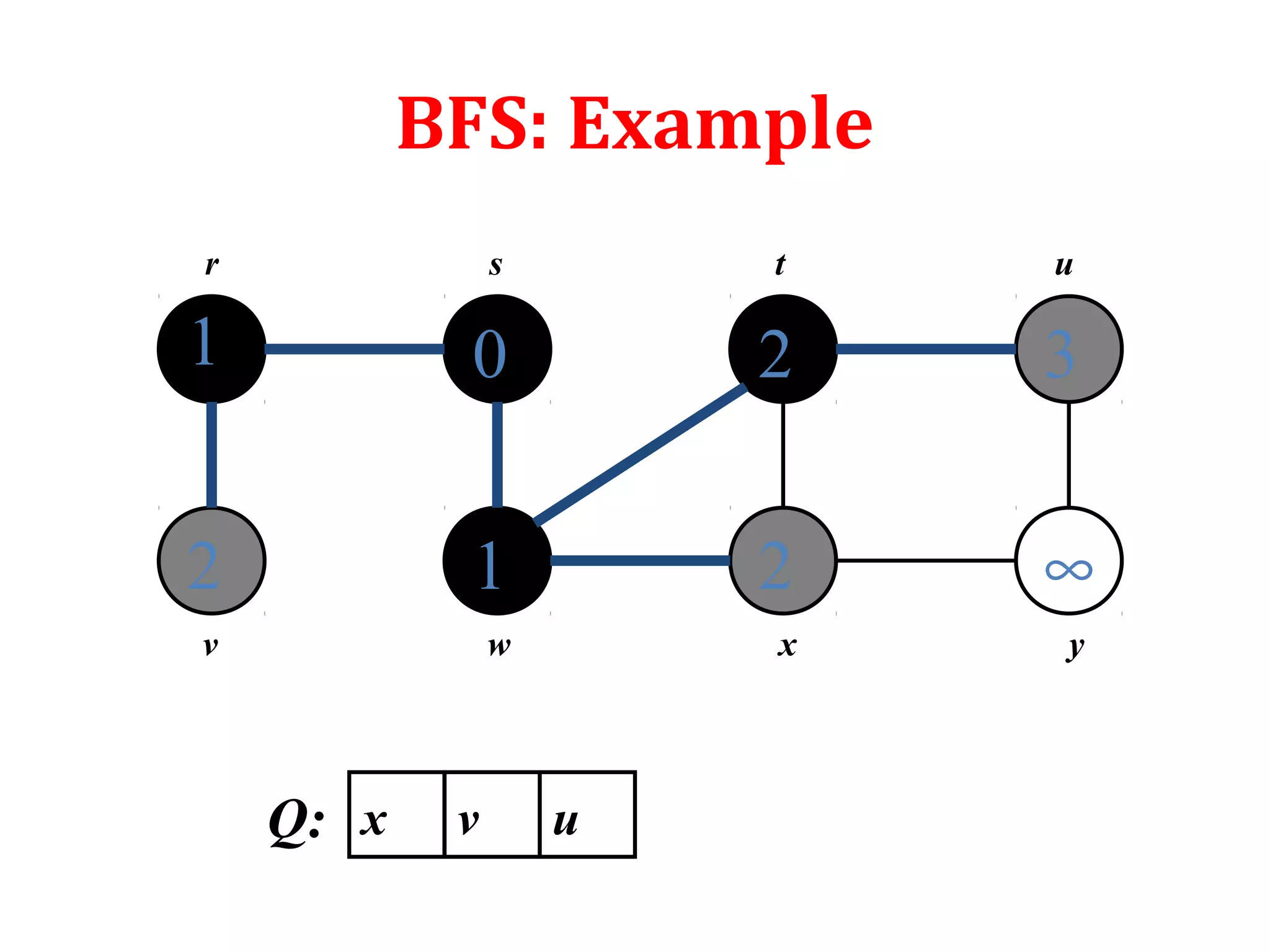
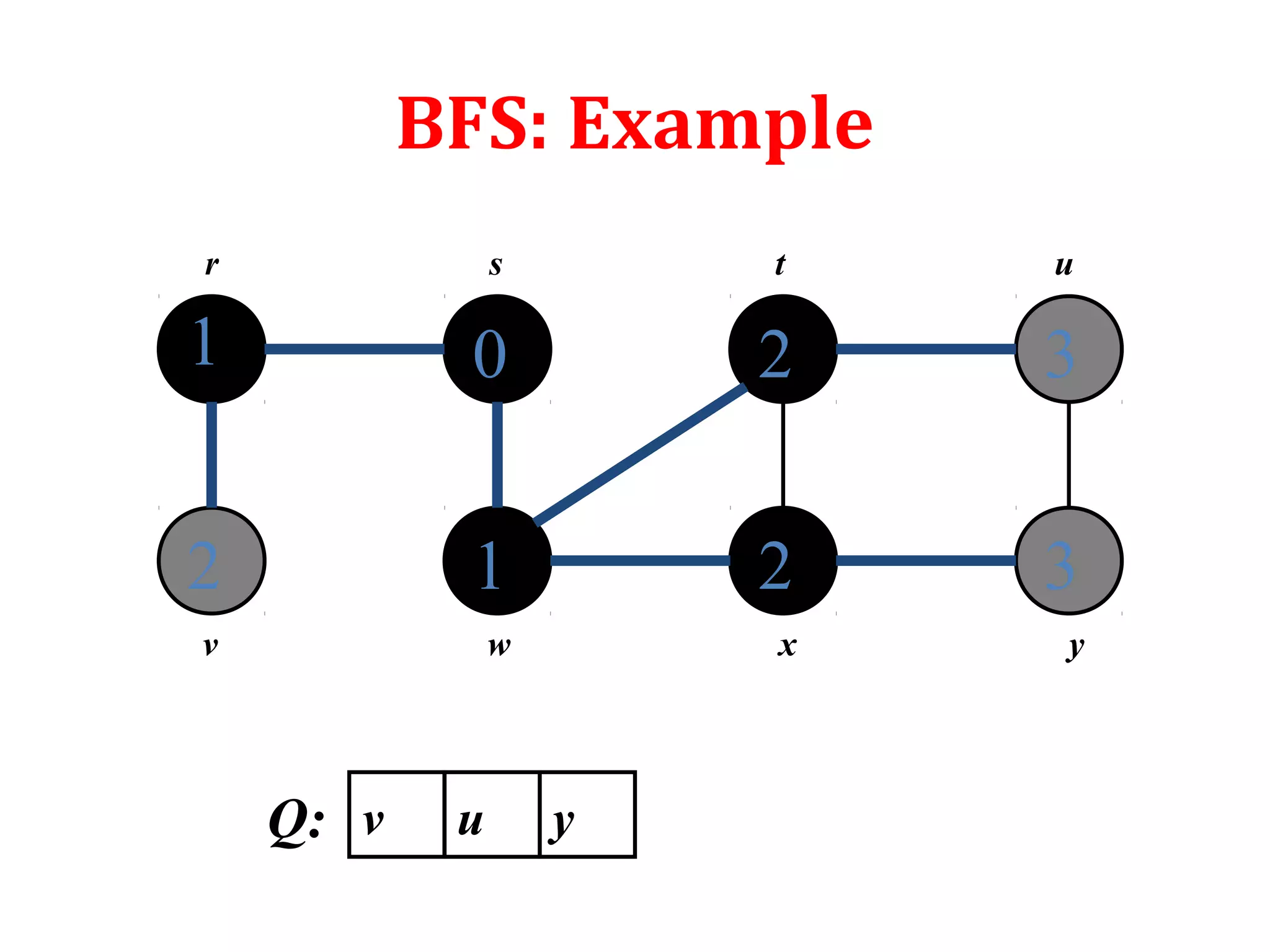
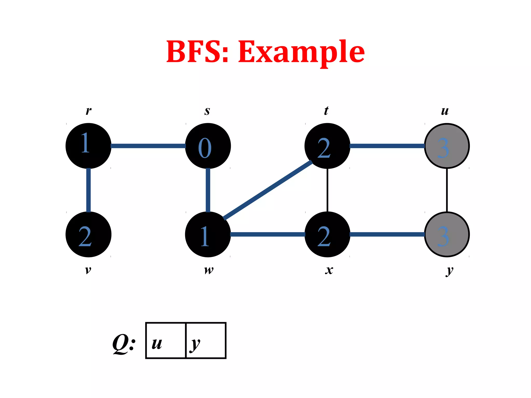
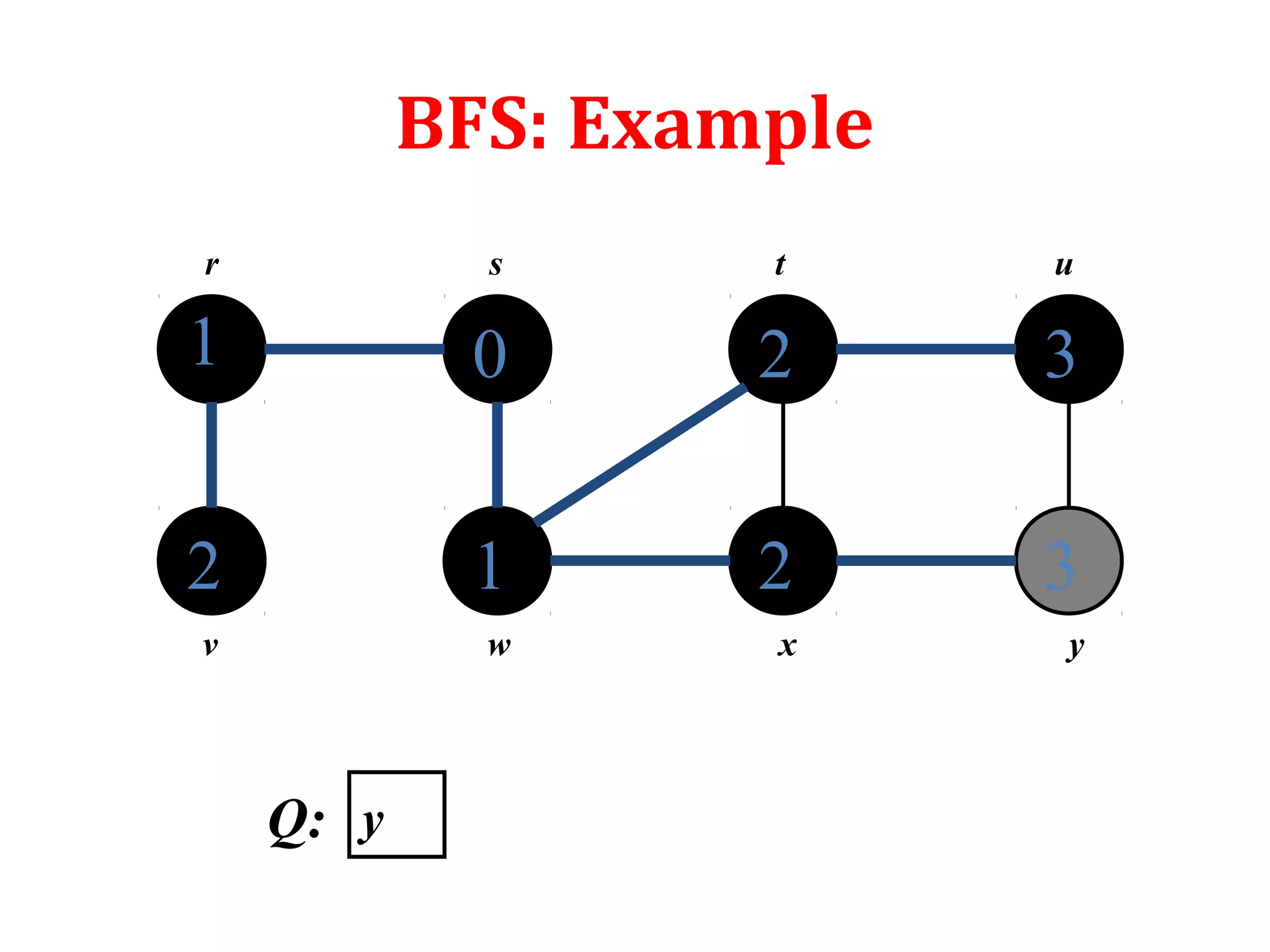
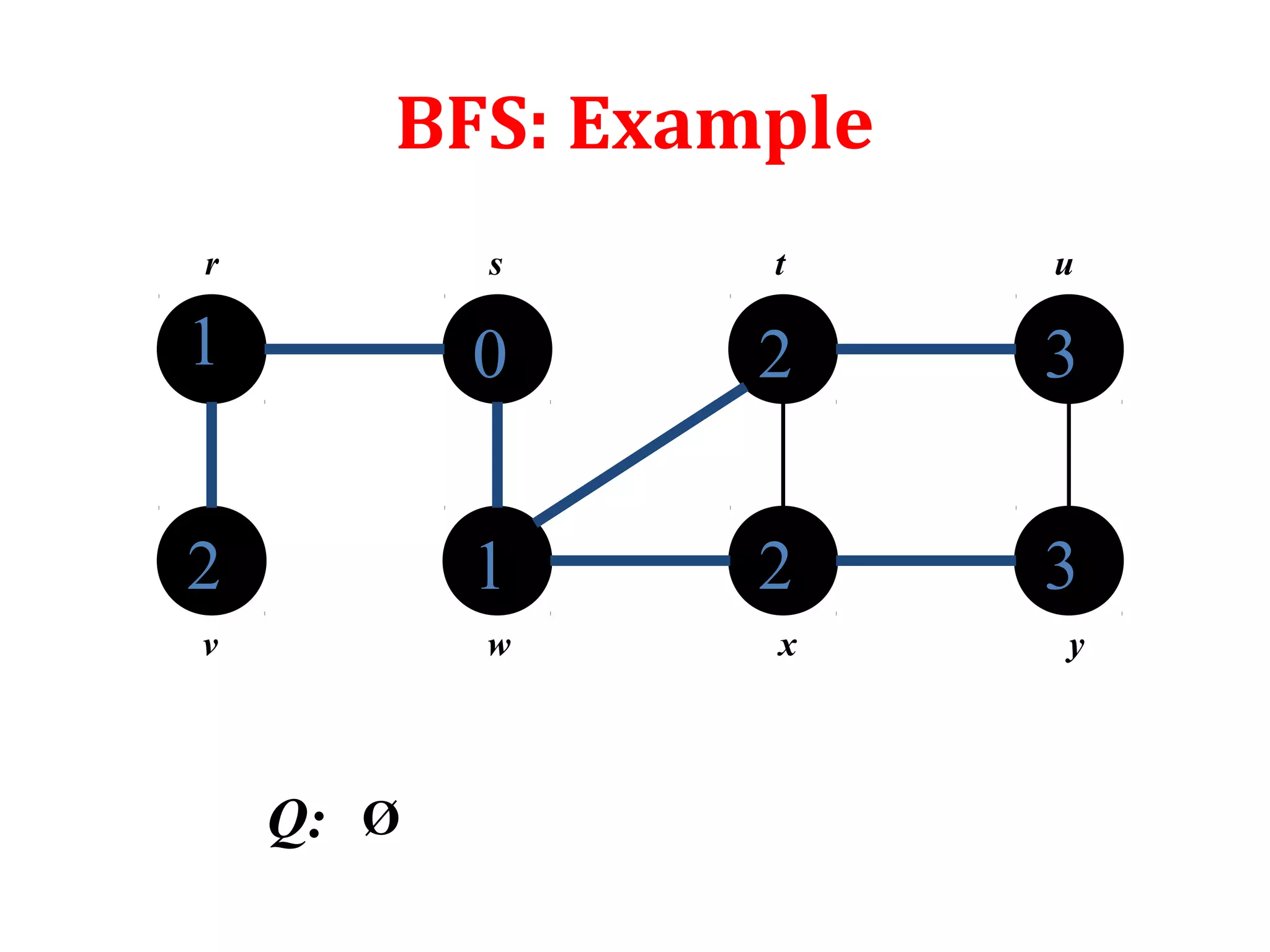
• It works for both directed and undirected graphs
• To keep track of progress BFS colors each vertex white,
gray or black. All vertices start with white and may later
become gray and then black. White color denote
undiscovered vertex. Gray and black denote discovered
vertex. While gray denote discovered vertex which is still
under process or in the queue. And black denote
completely processed and discovered vertex.
• d[u] denotes the distance of vertex u from source s
• (u) denotes the parent of vertexᴨ u
• Adj[u] denotes the adjacent vertices of u](https://image.slidesharecdn.com/bfs-dfs-170816093459/75/Breadth-first-search-and-depth-first-search-4-2048.jpg)
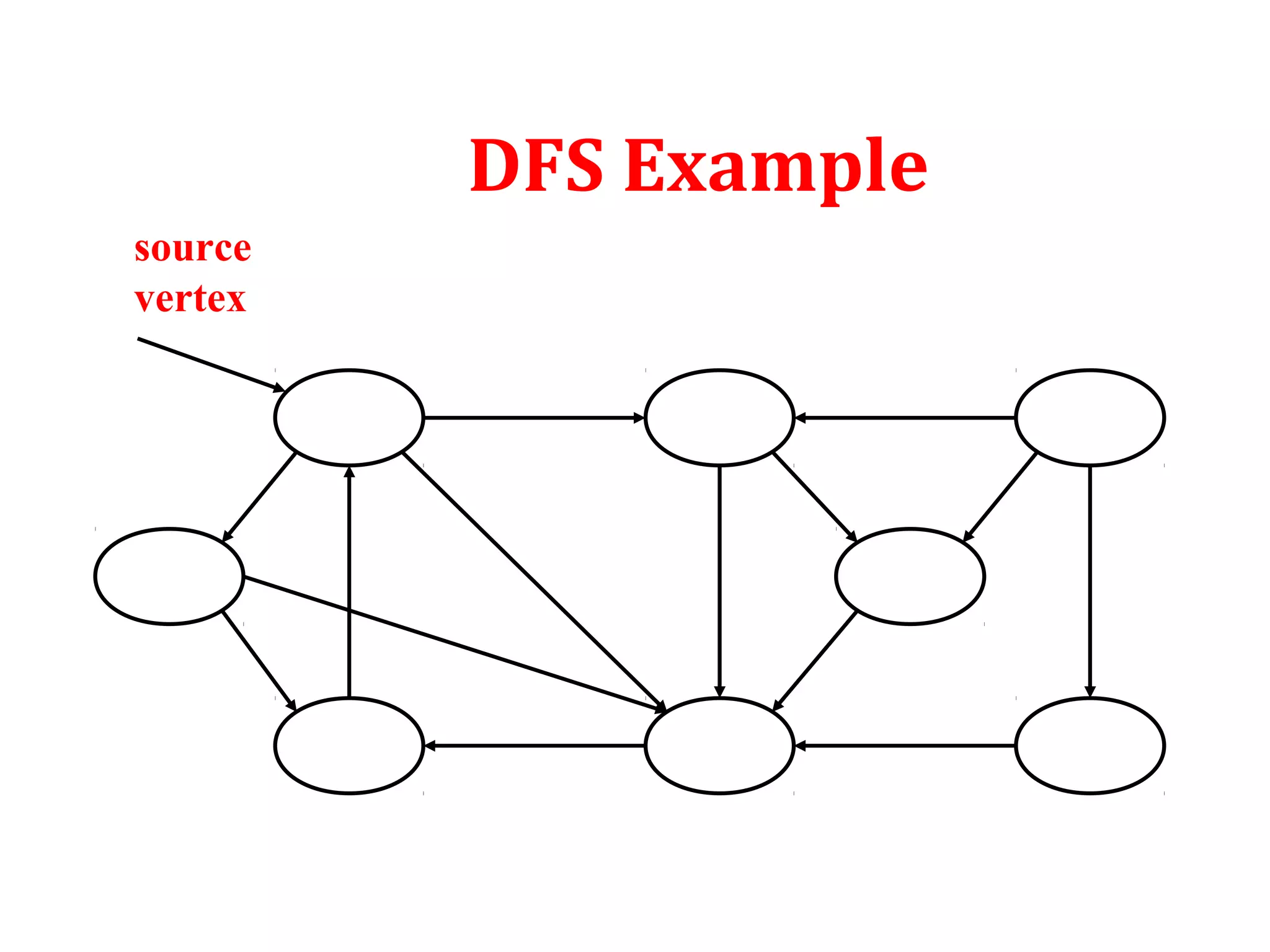
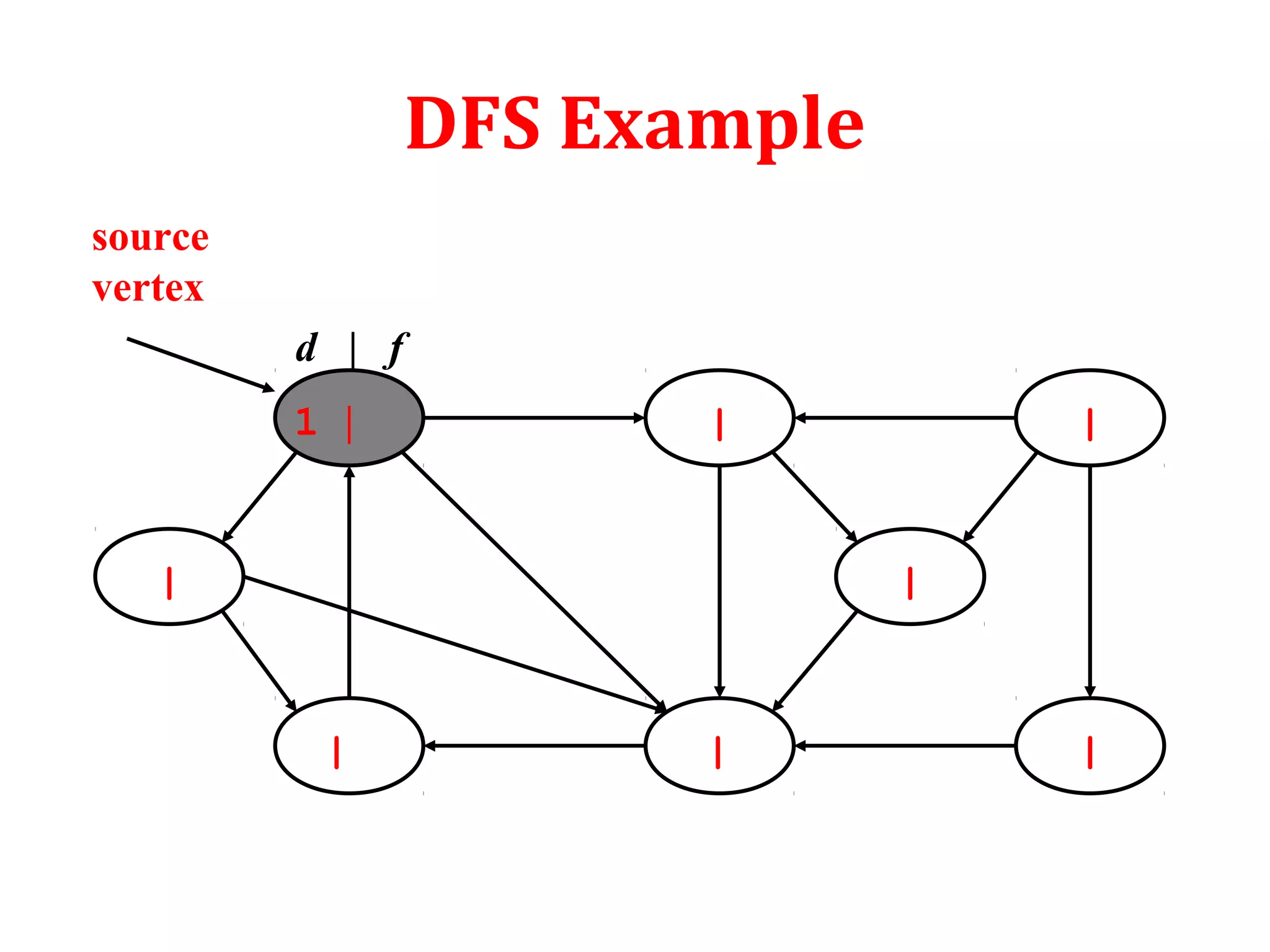
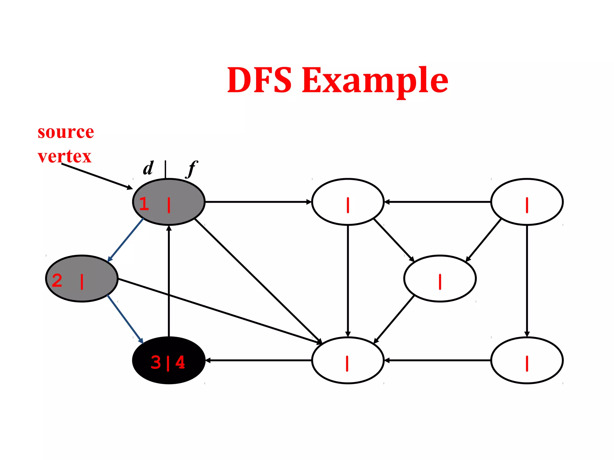
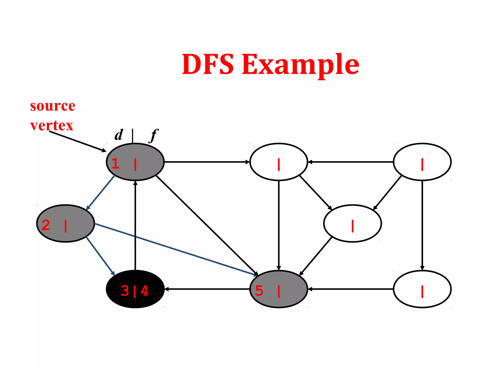
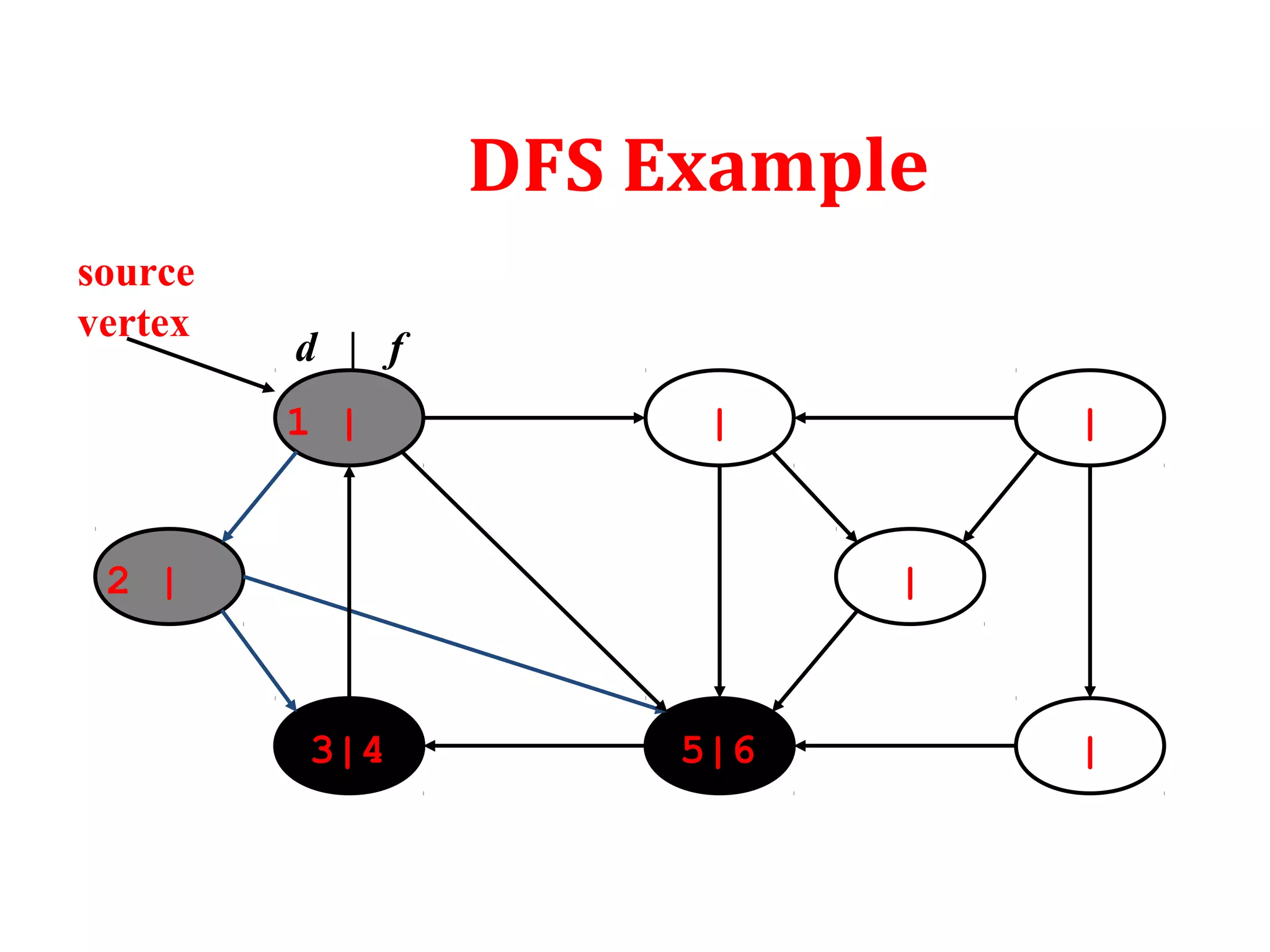
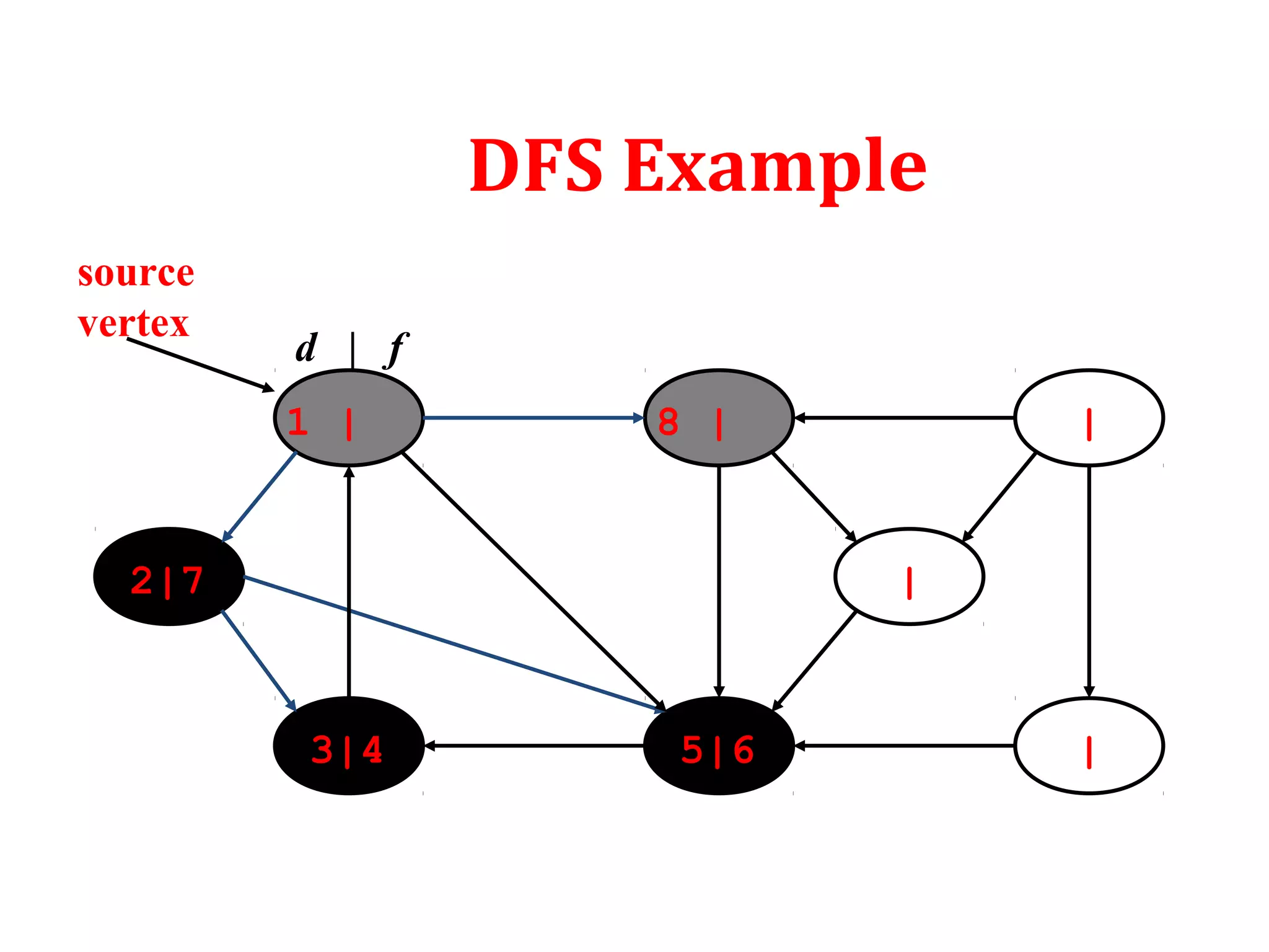
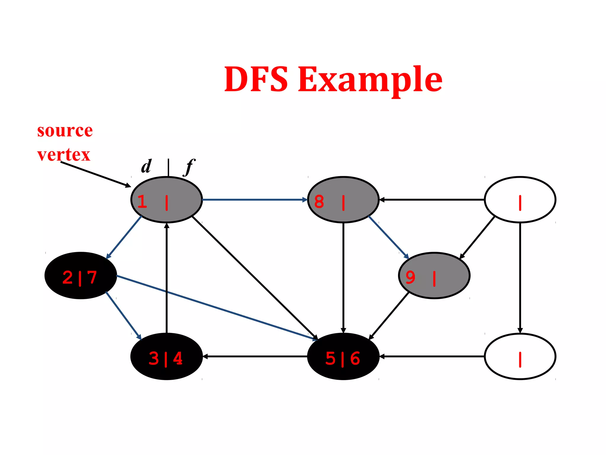
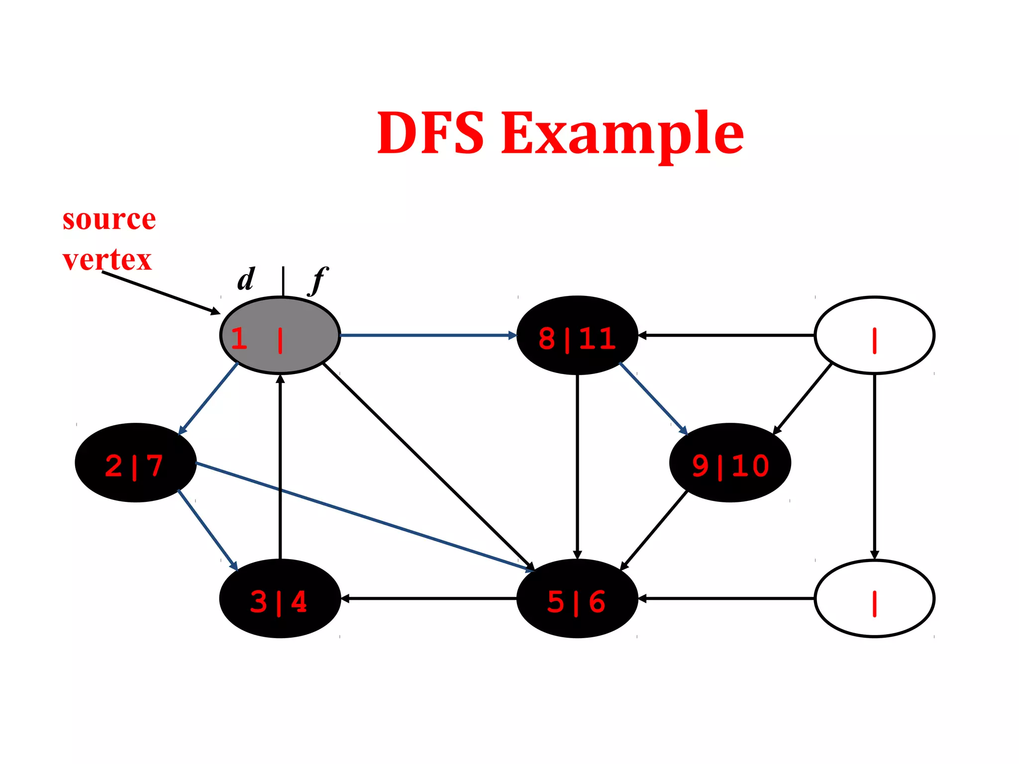
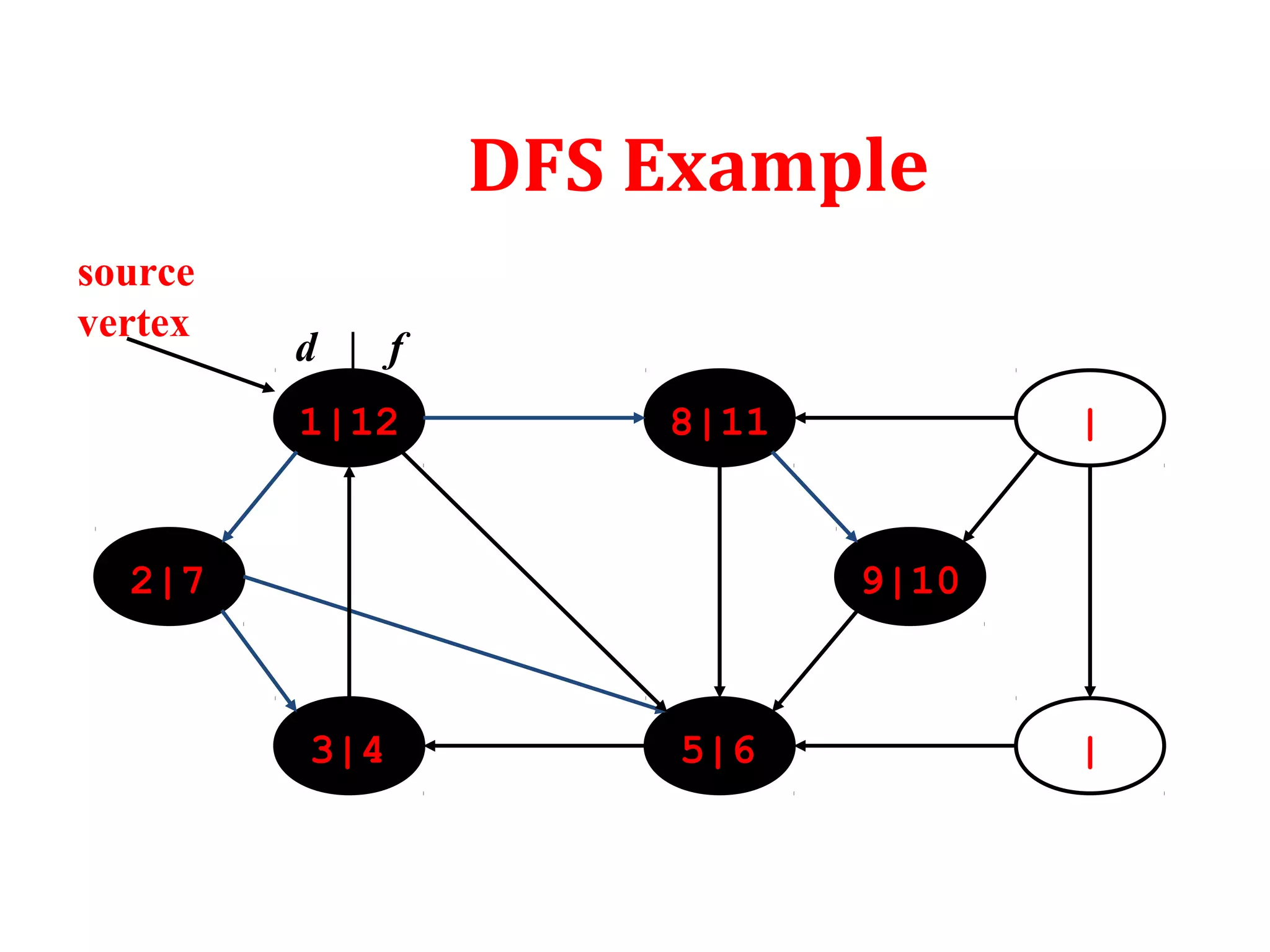
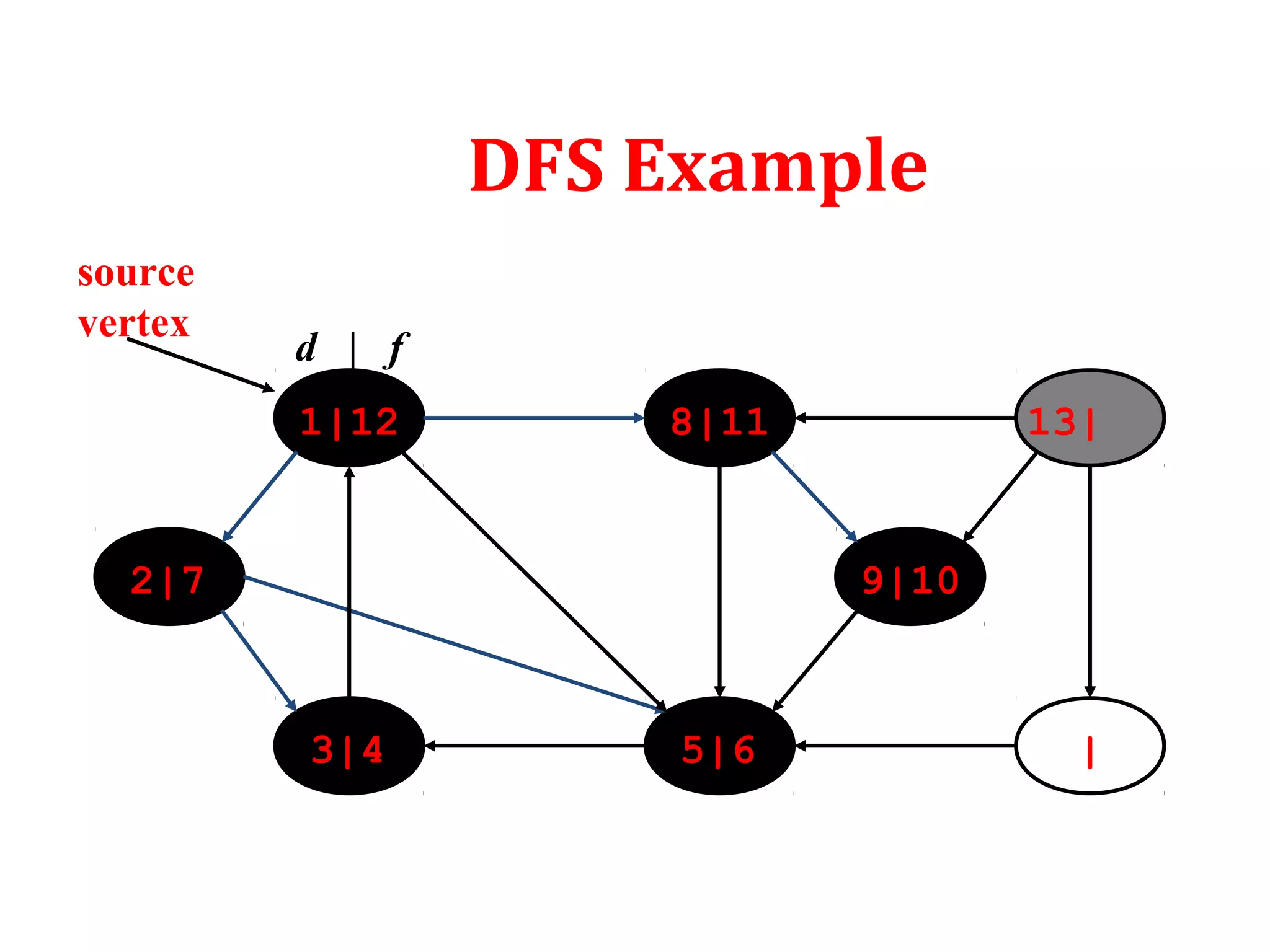
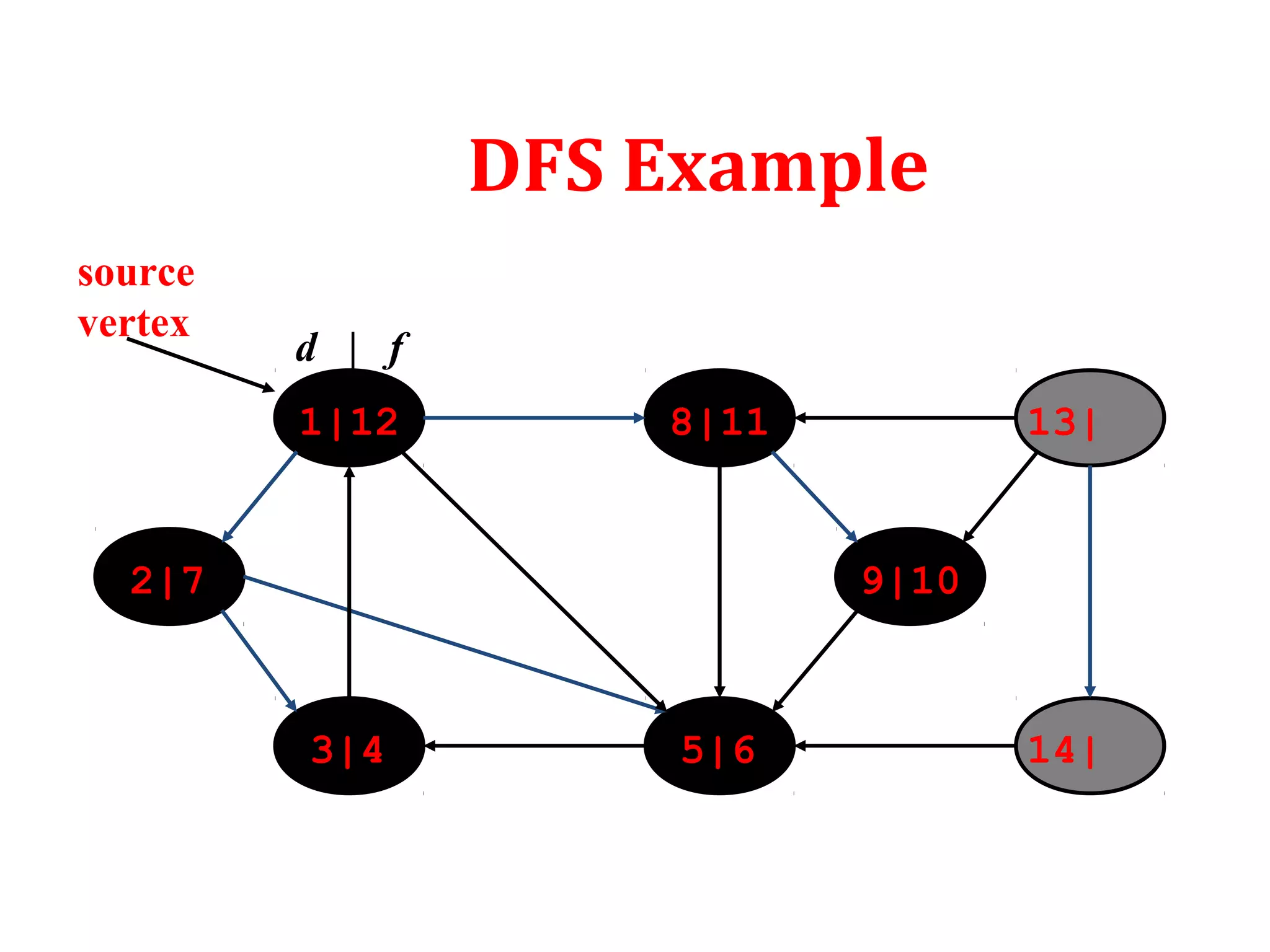
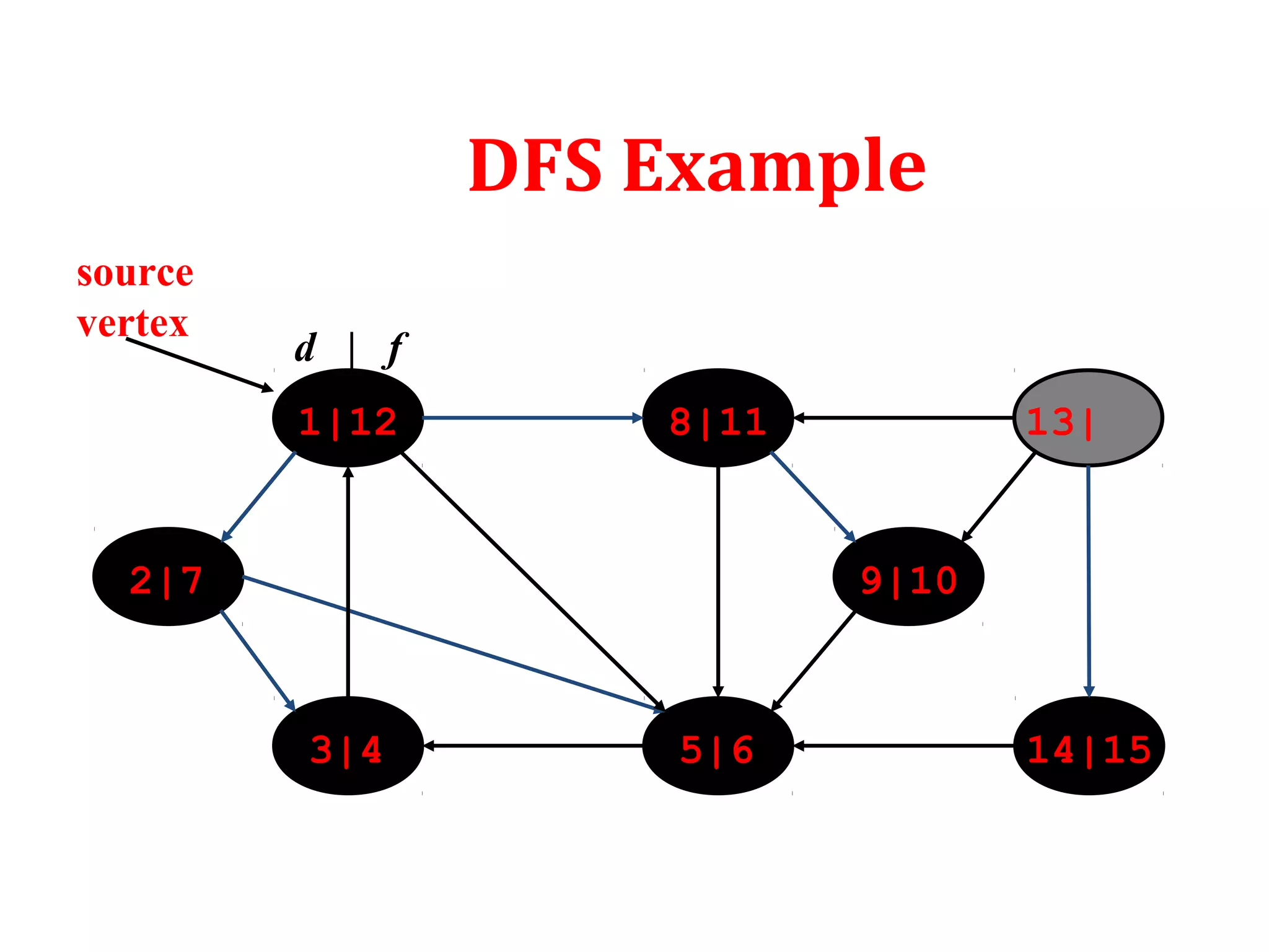
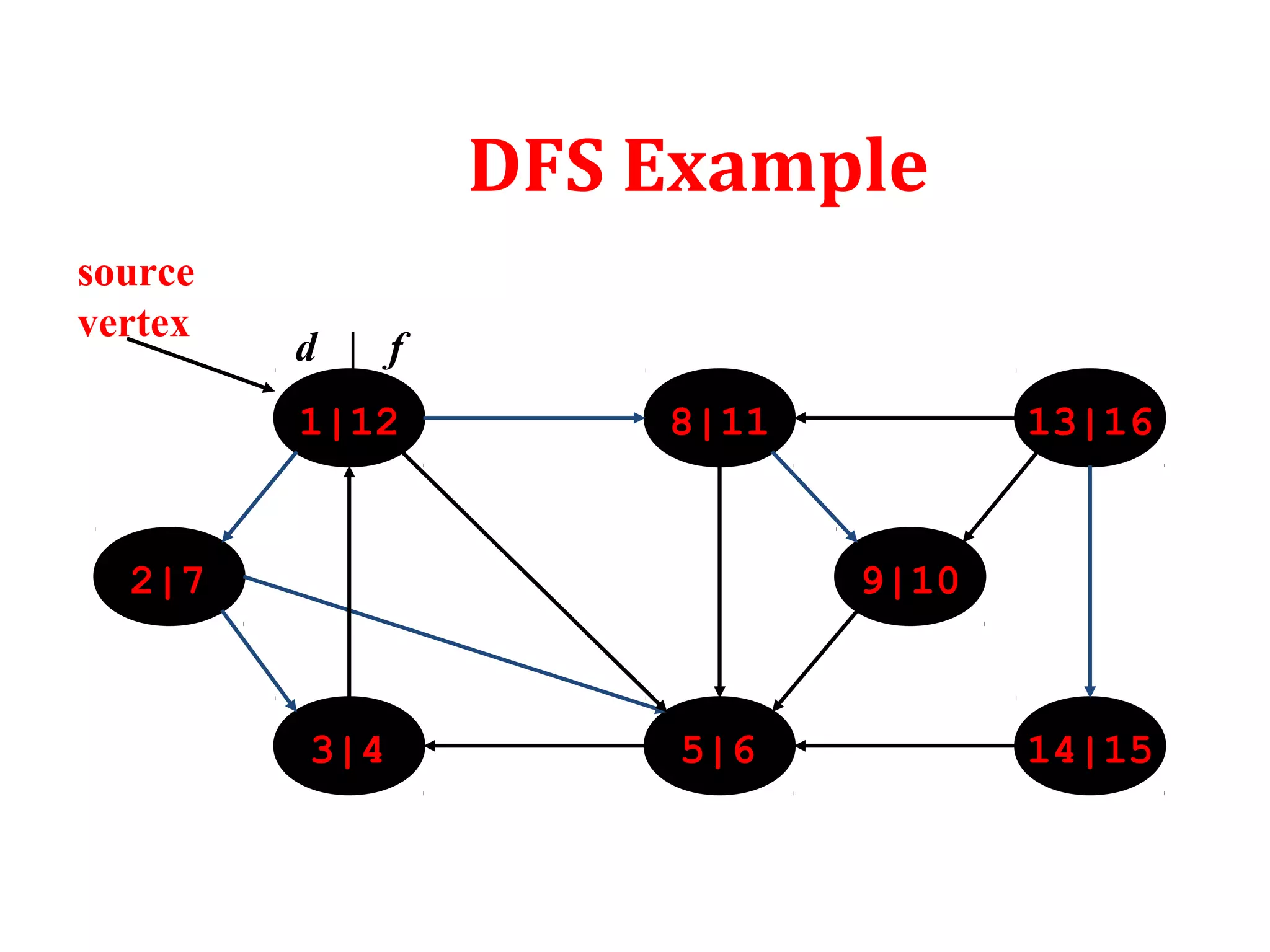
![Depth First Search
To keep track of progress DFS colors each vertex white, gray or
black. Initially all the vertices are colored white. Then they are
colored gray when discovered. Finally colored black when
finished.
Besides creating depth first forest DFS also timestamps each
vertex. Each vertex goes through two time stamps:
Discover time d[u]: when u is first discovered
Finish time f[u]: when backtrack from u or finished u
f[u] > d[u]](https://image.slidesharecdn.com/bfs-dfs-170816093459/75/Breadth-first-search-and-depth-first-search-21-2048.jpg)
![DFS: Algorithm
DFS(G)
1. for each vertex u in G
2. color[u]=white
3. [u]=NILᴨ
4. time=0
5. for each vertex u in G
6. if (color[u]==white)
7. DFS-VISIT(G,u)](https://image.slidesharecdn.com/bfs-dfs-170816093459/75/Breadth-first-search-and-depth-first-search-22-2048.jpg)
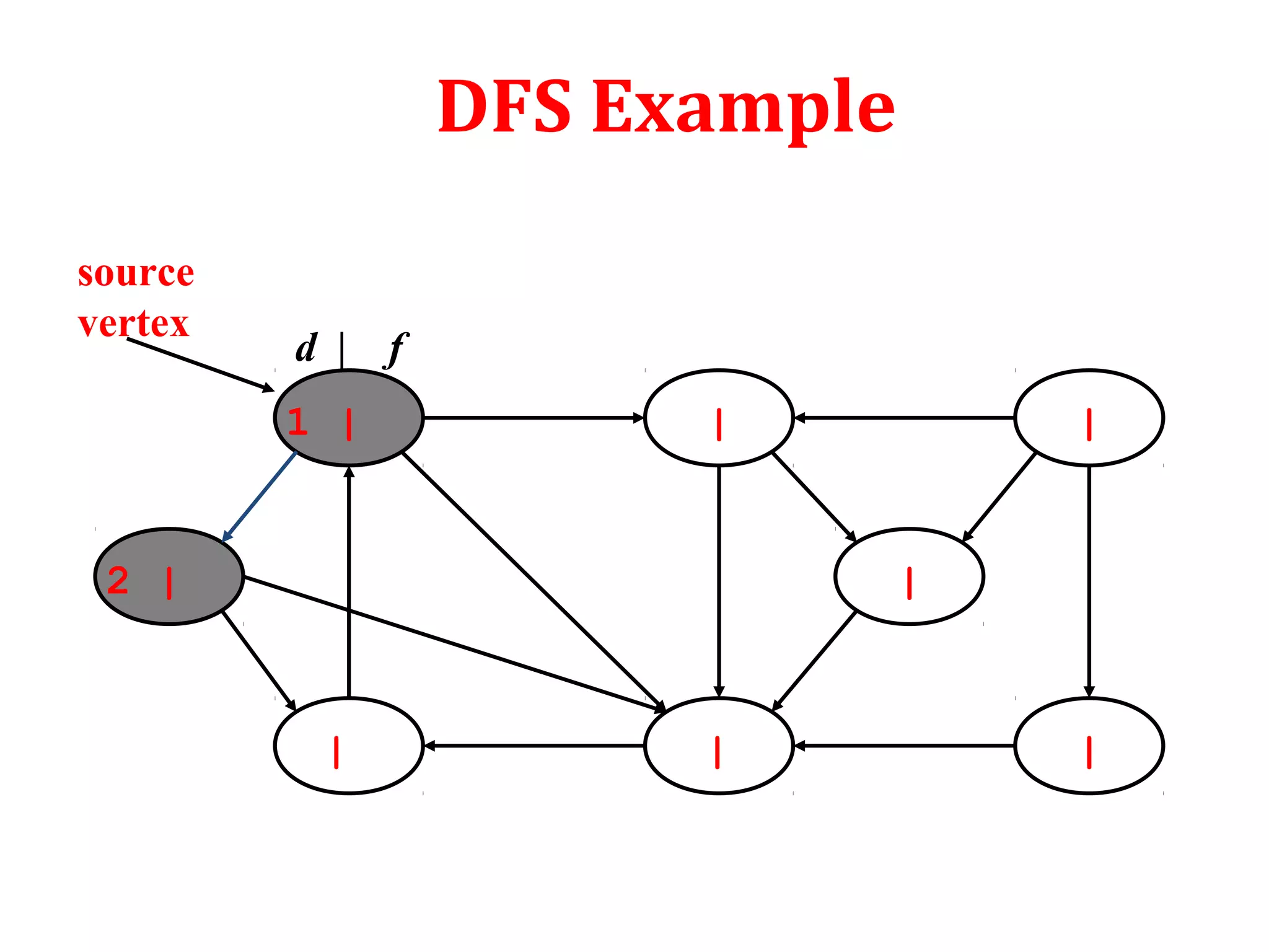
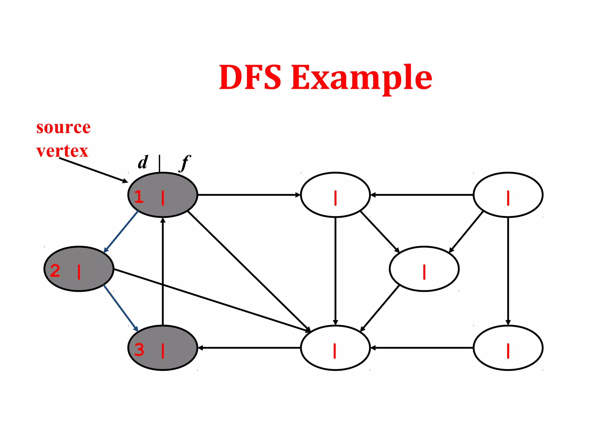
![DFS-VISIT(u)
1. time = time + 1
2. d[u] = time
3. color[u]=gray
4. for each v € Adj(u) in G do
5. if (color[v] = =white)
6. [v] = u;ᴨ
7. DFS-VISIT(G,v);
8. color[u] = black
9. time = time + 1;
10. f[u]= time;
DFS: Algorithm (Cont.)
source
vertex](https://image.slidesharecdn.com/bfs-dfs-170816093459/75/Breadth-first-search-and-depth-first-search-23-2048.jpg)


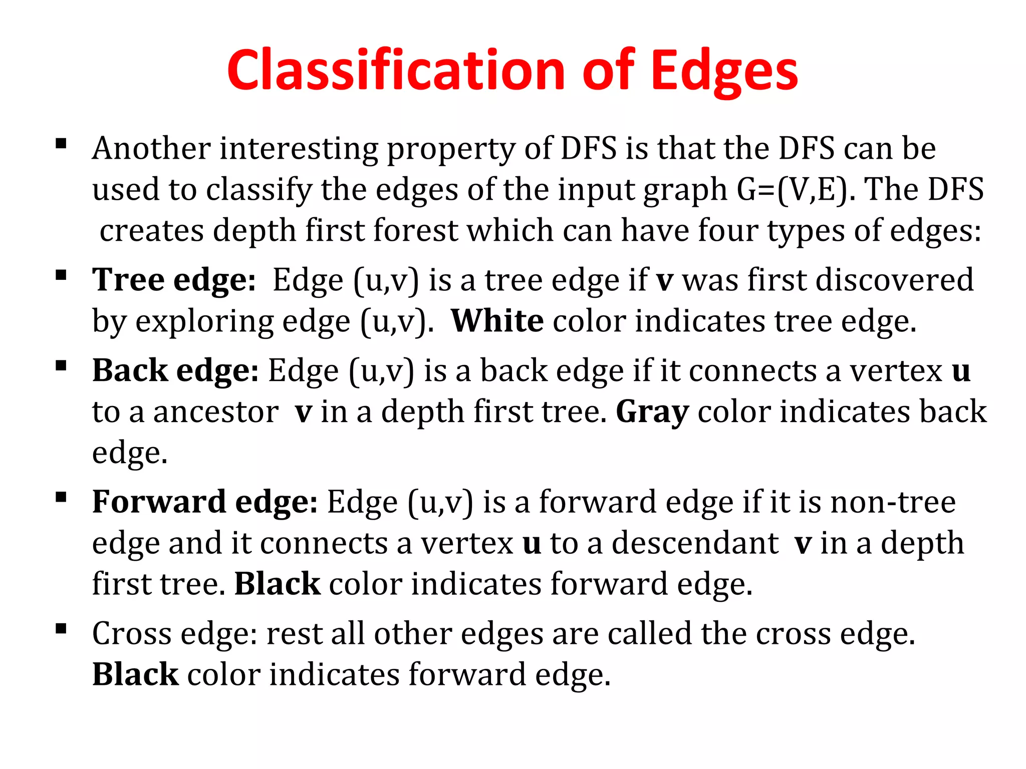


The document discusses two fundamental graph search algorithms: Breadth-First Search (BFS) and Depth-First Search (DFS). BFS systematically explores a graph level by level to find the shortest paths from a source vertex, while DFS explores as far as possible along branches before backtracking. Both algorithms utilize vertex coloring to keep track of their progress and have a time complexity of O(v + e), where v is the number of vertices and e is the number of edges.


![Depth first search [dfs]](https://cdn.slidesharecdn.com/ss_thumbnails/depthfirstsearchdfs-190926145304-thumbnail.jpg?width=640&height=640&fit=bounds)