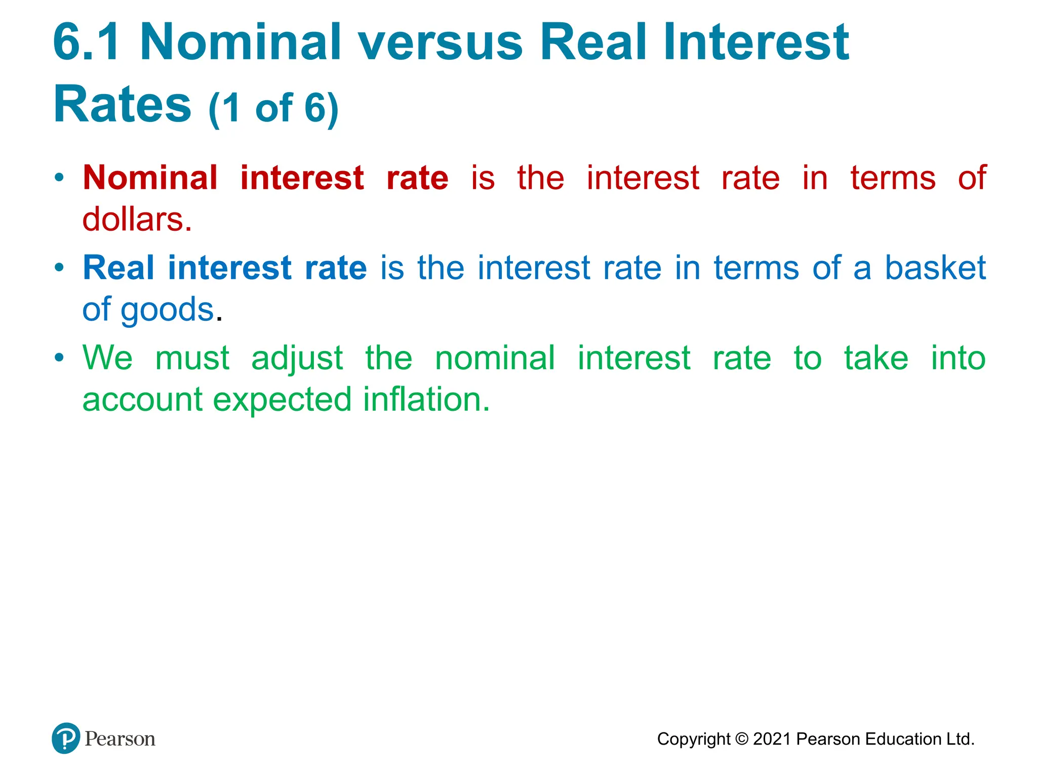
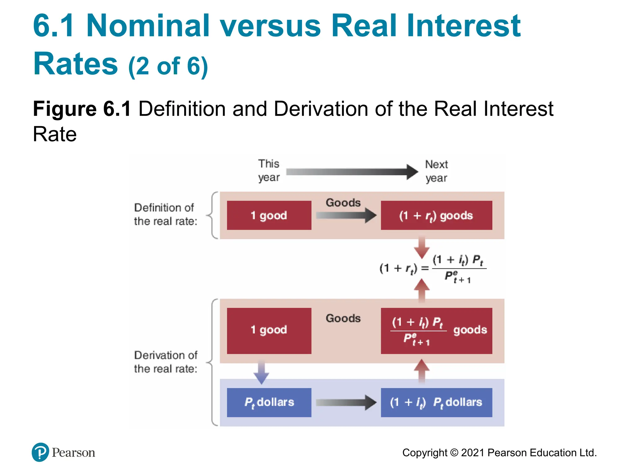
Macroeconomics
Eighth Edition, Global Edition
Chapter 6
Financial Markets II: The Extended
IS-LM Model
• Copyright © 2021 Pearson Education Ltd.
Slide in this Presentation Contain Hyperlinks.
JAWS users should be able to get a list of links
by using INSERT+F7
Copyright © 2021 Pearson Education Ltd.
Chapter 6 Outline
Financial Markets II: The Extended IS-LM Model
6.1 Nominal versus Real Interest Rates
6.2 Risk and Risk Premia
6.3 The Role of Financial Intermediaries
6.4 Extending the IS-LM Model
6.5 From a Housing Problem to a Financial Crisis
Copyright © 2021 Pearson Education Ltd.
Financial Markets II: The Extended
IS-LM Model
• Until now, we assumed that there were only two financial
assets—money and bonds—and just one interest rate—
the rate on bonds—determined by monetary policy.
• The financial system also plays a major role in the
economy.
• This chapter looks more closely at the role of the financial
system and its macroeconomic implications.
Copyright © 2021 Pearson Education Ltd.
6.1 Nominal versus Real Interest
Rates (1 of 6)
• Nominal interest rate is the interest rate in terms of
dollars.
• Real interest rate is the interest rate in terms of a basket
of goods.
• We must adjust the nominal interest rate to take into
account expected inflation.
Copyright © 2021 Pearson Education Ltd.
6.1 Nominal versus Real Interest
Rates (2 of 6)
Figure 6.1 Definition and Derivation of the Real Interest
Rate
Copyright © 2021 Pearson Education Ltd.
6.1 Nominal versus Real Interest
Rates (3 of 6)
• One-year real interest rate rt:
1 + 𝑟𝑡 = 1 + 𝑖𝑡
𝑃t
𝑝𝑡+1
𝑒 (6.1)
• Denote expected inflation between t and t + 1 by:
𝜋𝑡+1
𝑒
=
(𝑃𝑡 +1
𝑒
− 𝑃t)
𝑝𝑡
(6.2)
so that equation (6.1) becomes
1 + 𝑟𝑡 =
1 + 𝑖𝑡
1 + 𝜋𝑡
𝑒 (6.3)
Copyright © 2021 Pearson Education Ltd.
6.1 Nominal versus Real Interest Rates
1 + 𝑟𝑡 = 1 + 𝑖𝑡
𝑃t
𝑃𝑡+1
𝑒
𝑃𝑡+1
𝑒
𝑃t
1 + 𝑟𝑡 = 1 + 𝑖𝑡
𝜋𝑡+1
𝑒
=
(𝑃𝑡 +1
𝑒
− 𝑃t)
𝑝𝑡
𝑃𝑡+1
𝑒
𝑃t
− 𝟏 + 𝟏 1 + 𝑟𝑡 = 1 + 𝑖𝑡
𝑃𝑡+1
𝑒
− 𝑃t
𝑃t
+ 𝟏 1 + 𝑟𝑡 = 1 + 𝑖𝑡
𝟏 + 𝝅𝒕+𝟏
𝒆
1 + 𝒓𝒕 = 1 + 𝑖𝑡
𝟏 + 𝝅𝒕+𝟏
𝒆
+ 𝒓𝒕 + 𝝅𝒕+𝟏
𝒆
𝒓𝒕
≈𝟎
= 1 + 𝒊𝒕
𝝅𝒕+𝟏
𝒆
+ 𝒓𝒕 ≈ 𝒊𝒕
𝒓𝒕 =
1 + 𝒊𝒕
𝝅𝒕+𝟏
𝒆
+ 𝟏
− 𝟏
Copyright © 2021 Pearson Education Ltd.
6.1 Nominal versus Real Interest Rates (4 of 6)
• If the nominal interest rate and expected inflation are not
too large, a close approximately to equation (6.3) is:
• When expected inflation equals zero, the nominal interest
rate and the real interest rate are equal.
• Because expected inflation is typically positive, the real
interest rate is typically lower than the nominal interest
rate.
• For a given nominal interest rate, the higher expected
inflation, the lower the real interest rate.
𝒓𝒕 ≈ 𝒊𝒕 − 𝝅𝒕+𝟏
𝒆
Copyright © 2021 Pearson Education Ltd.
𝒓𝒕 =
1 + 𝑖𝑡
𝝅𝒕+𝟏
𝒆
+ 𝟏
− 1
𝒓𝒕 ≈ 𝒊𝒕 − 𝝅𝒕+𝟏
𝒆
Reel Interest Rate
𝒓𝒕 =
1 + 𝑖𝑡
𝝅𝒕+𝟏
𝒆
+ 𝟏
− 1
𝒓𝒕 ≈ 𝒊𝒕 − 𝝅𝒕+𝟏
𝒆
𝑖𝑡=10%
𝝅𝒕+𝟏
𝒆
= 𝟓% 𝒓𝒕 = 𝟎, 𝟎𝟒𝟕𝟔 ≈ 𝟒, 𝟖% 𝒓𝒕 ≈ 𝟓%
𝑖𝑡=100%
𝝅𝒕+𝟏
𝒆
= 𝟖𝟎% 𝒓𝒕 = 𝟎, 𝟏𝟏𝟏 ≈ 𝟏𝟏% 𝒓𝒕 ≈ 𝟐𝟎%
6.1 Nominal versus Real Interest Rates
Copyright © 2021 Pearson Education Ltd.
6.1 Nominal versus Real Interest Rates (5 of 6)
• The interest rate that enters the IS relation is the real
interest rate. Spending and saving decisions depend on
expected inflation rate.
• Zero lower bound: The nominal interest rate cannot go
below zero.
• The zero lower bond of the nominal interest rate implies that
the real interest rate cannot be lower than the negative of
inflation.
Copyright © 2021 Pearson Education Ltd.
6.1 Nominal versus Real Interest
Rates (6 of 6)
Figure 6.2 Nominal and Real One-Year T-Bill Rates in the United States since
1978
The nominal interest rate has declined considerably since the early 1980s, but
because expected inflation has declined as well, the real rate has declined much
less than the nominal rate.
𝒓𝒕 ≈ 𝒊𝒕 − 𝝅𝒕+𝟏
𝒆
Copyright © 2021 Pearson Education Ltd.
6.1 Nominal versus Real Interest Rates
• The real interest rate (i − πe) is based on expected inflation,
so it is sometimes called the ex-ante (“before the fact”) real
interest rate.
• The realized real interest rate (i − π) is called the ex-post
(“after the fact”) interest rate.
Although the central bank chooses the nominal rate (as we saw in
Chapter 4), it cares about the real interest rate because this is the
rate that affects spending decisions. To set the real interest rate it
wants, it thus has to take into account expected inflation. For
example, if it wants the real interest rate to be 4% and expected
inflation is 2%, it will set the nominal interest rate, i, at 6%.
𝒓𝒕 ≈ 𝒊𝒕 − 𝝅𝒕+𝟏
𝒆
Copyright © 2021 Pearson Education Ltd.
6.2 Risk and Risk Premia
• Some bonds are risky, so bond holders require a risk premium.
• Let i be the nominal interest rate on a riskless bond, x be
the risk premium, and p is the probability of defaulting,
then to get the same expected return on the risky bonds as
on the riskless bond:
(1 + i) = (1 – p)(1 + i + x) + (p)(0)
Risk premia are determined by:
The probability of default
Nominal government bonds interest rate
Another second factor is the degree of risk aversion of the bond holders
Copyright © 2021 Pearson Education Ltd.
6.2 Risk and Risk Premia
Copyright © 2021 Pearson Education Ltd.
6.2 Risk and Risk Premia
Figure 6.3 Yields on 10-Year U.S. Government Treasury,
AAA, and BBB Corporate Bonds, since 2000
In September 2008, the financial crisis led to a sharp
increase in the rates at which firms could borrow.
• Source: FRED: Series DGS10; For AAA and BBB corporate bonds, Bank of America Merrill Lynch
Series BAMLC0A4CBBB, BAMLC0A1CAAAEY.
Copyright © 2021 Pearson Education Ltd.
Policy Rate
Federal Funds
Rate
Government Bonds
Rate
i
Corporate Bonds
Rate
i+𝒙
nominal interest rate on a
riskless bond and risk premium.
6.2 Risk and Risk Premia
Copyright © 2021 Pearson Education Ltd.
6.3 The Role of Financial Intermediaries
• Until now, we have looked at direct finance—borrowing directly by the
ultimate borrowers from the ultimate lenders.
• In fact, much of the borrowing and lending takes place through financial
intermediaries—financial institutions that receive funds from
investors and then lend these funds to others.
• “Shadow banking, the nonbank part of the financial system
mortgage companies, money market funds, and hedge funds.
Copyright © 2021 Pearson Education Ltd.
• Financial intermediaries (Mostly Banks): Institutions that
receive funds from people and firms and use these
funds to buy financial assets or to make loans to other
people and firms.
• Banks are financial intermediaries that have money, in
the form of checkable deposits, as their liabilities.
• Banks keep as reserves some of the funds (deposits)
they receive.
6.3 The Role of Financial Intermediaries
Copyright © 2021 Pearson Education Ltd.
𝑫𝒆𝒑𝒐𝒔𝒊𝒕𝒔 = 𝟐𝟎𝟎 → 𝑹𝒆𝒔𝒆𝒓𝒗𝒆 𝑹𝒂𝒕𝒊𝒐 %10 𝑹𝒆𝒔𝒆𝒓𝒗𝒆𝒔 = 𝟐𝟎
↓
𝟏𝟖𝟎
𝑪𝒓𝒆𝒂𝒕𝒊𝒏𝒈 𝑳𝒐𝒂𝒏𝒔 𝑩𝒖𝒚𝒊𝒏𝒈 𝑨𝒔𝒔𝒆𝒕𝒔 (𝑩𝒐𝒏𝒅𝒔)
Copyright © 2021 Pearson Education Ltd.
Central Bank
Assets Liabilities
Bonds Currency
Reserves 8
Banks
Assets Liabilities
Reserves 8 Deposits 80
Bonds 42 Capital 20
Loans 50
ณ
𝜽
𝑹𝒆𝒒𝒖𝒊𝒓𝒆𝒅
𝑹𝒆𝒔𝒆𝒓𝒗𝒆
𝑹𝒂𝒕𝒊𝒐
= 𝟏𝟎%
Copyright © 2021 Pearson Education Ltd.
6.3 The Role of Financial Intermediaries
Figure 6.4 Bank Assets, Capital, and Liabilities
• Capital ratio (the ratio of capital to assets) = 20/100 = 20%
• Leverage ratio (the ratio of assets to capital) = 100/20 = 5
A higher leverage ratio implies a higher expected profit rate,
but also implies a higher risk of insolvency and bankruptcy.
Consider a bank that has assets of 100, liabilities of 80, and capital of 20. You can
think of the owners of the bank as having directly invested 20 of their own
funds, borrowed another 80 from other investors, and bought various assets
for 100. The liabilities may be checkable deposits, interest-paying deposits, or
borrowing from investors and other banks. The assets may be reserves (central
bank money), loans to consumers, loans to firms, loans to other banks,
mortgages, government bonds, or other forms of securities
Copyright © 2021 Pearson Education Ltd.
6.3 The Role of Financial
Intermediaries
The Choice of Leverage
Why shouldn’t the bank choose a high
leverage ratio?
Because higher leverage also implies a
higher risk that the value of the assets
becomes less than the value of liabilities, in
turn implying a higher risk of insolvency.
𝑳𝒆𝒗𝒆𝒓𝒂𝒈𝒆 𝑹𝒂𝒕𝒊𝒐 𝟓 ⇛ 𝟏𝟎
𝑨𝒔𝒔𝒆𝒕𝒔 𝟏𝟎𝟎 ⇛ 𝟏𝟎𝟎
𝑳𝒊𝒂𝒃𝒊𝒍𝒊𝒕𝒊𝒆𝒔 𝟖𝟎 ⇛ 𝟗𝟎
Bank Balance Sheet
Assets 100 Liabilities 80 ⇛ 90
Capital 20 ⇛ 10
For the bank its assets can decrease in value to 80 without the bank
becoming insolvent and going bankrupt. But if it were to choose a leverage
ratio of 10, any decrease in the value of the assets below 90 would lead the
bank to become insolvent. The risk of bankruptcy would be much higher.
Thus, the bank must choose a leverage ratio that takes into account both
factors. Too low a leverage ratio means less profit. Too high a leverage ratio
means too high a risk of bankruptcy.
Copyright © 2021 Pearson Education Ltd.
FOCUS: Bank Runs
• The U.S. financial history up to the 1930s is full of bank
runs.
• One potential solution to bank runs is narrow banking,
which restricts banks from making loans, and to hold liquid
and safe government bonds.
• To limit bank runs, the United States introduced federal
deposit insurance in 1934.
• The Fed also implemented liquidity provision so that
banks could borrow overnight from other financial
institutions.
Copyright © 2021 Pearson Education Ltd.
What Happened to SVB Bank?(March 2023)
• At the root of the recent crisis was uninsured deposits of
the Silicon Valley Bank (SVB).
• As the Fed sharply tightened monetary policy to control
inflation, companies found it more difficult to raise cash,
leading to deposit outflows. To meet those outflows, SVB
sold long-term Treasuries it held on its balance
sheet—the value of which had plummeted as interest
rates rose—at a loss. A capital raise to cover those losses
failed, and a significant run on deposits occurred,
resulting in the largest bank failure since the 2008 financial
crisis.
• This prompted a broad migration of deposits out of the
banking system, forcing some banks to source liquidity
from the Fed.
Copyright © 2021 Pearson Education Ltd.
6.4 Extending the IS-LM Model (1 of 4)
• Now we extend the IS-LM to reflect the distinction
between:
1. the nominal interest rate and the real interest rate
2. the policy rate set by the central bank and the interest
rates faced by borrowers
• Rewrite the IS-LM:
IS relation: 𝒀 = 𝑪(𝒀 − 𝑻) + 𝑰(𝒀, 𝒊 − 𝝅𝒆
𝒓
+ 𝒙) + 𝑮
LM relation: 𝒊 = 𝒊
where expected inflation πe and the risk premium x enter
the IS relation.
Copyright © 2021 Pearson Education Ltd.
Policy interest rate
Short Run
(overnight) Money
Market interest rate
Loan and deposit
interest rates
Government and
Corporate Bonds
Market interest rate
Copyright © 2021 Pearson Education Ltd.
6.4 Extending the IS-LM Model (2 of 4)
• The central bank now chooses the real policy rate r,
which enters the IS equation as part of the borrowing rate
(r + x) for consumers and firms:
IS relation: 𝒀 = 𝑪 𝒀 − 𝑻 + 𝑰 𝒀, 𝒓 + 𝒙 + 𝑮 (𝟔. 𝟓)
LM relation: 𝒓 = 𝒓 (𝟔. 𝟔)
Copyright © 2021 Pearson Education Ltd.
6.4 Extending the IS-LM Model (3 of 4)
Figure 6.5 Financial Shocks and Output
An increase in x leads to a shift of the IS curve to the left and
a decrease in equilibrium output.
Copyright © 2021 Pearson Education Ltd.
6.4 Extending the IS-LM Model
Figure 6.6 Financial Shocks, Monetary Policy, and Output
If sufficiently large, a decrease in the policy rate can in principle
offset the increase in the risk premium.
The zero lower bound
may however put a
limit on the decrease
in the real policy rate.
Alternative policy could have been a fiscal
expansion. But a large increase in spending or a
cut in taxes may imply a large increase in the
budget deficit, and the government may be
reluctant to cause this.
𝒓𝒕 ≈ 𝒊𝒕 − 𝝅𝒕+𝟏
𝒆
Copyright © 2021 Pearson Education Ltd.
6.5 From a Housing Problem to a
Financial Crisis (1 of 10)
Figure 6.7 U.S. Housing Prices since 2000
The increase in housing prices from 2000 to 2006 was
followed by a sharp decline thereafter.
Source: FRED: Case-Shiller Home Price Indices, 10-city home price index, Series
SPCS10RSA
Copyright © 2021 Pearson Education Ltd.
6.5 From a Housing Problem to a
Financial Crisis (2 of 10)
• The 2000s were a period of unusually low interest rates,
which stimulated housing demand.
• Mortgage lenders was increasingly willing to make loans to
risky borrowers with subprime mortgages, or subprimes.
• From 2006 on, many home mortgages went underwater
(when the value of the mortgage exceeded the value of the
house).
• Lenders faced large losses as many borrowers defaulted.
Copyright © 2021 Pearson Education Ltd.
6.5 From a Housing Problem to a
Financial Crisis (3 of 10)
• Banks were highly leveraged because:
– Banks probably underestimated the risk,
– Bank managers had incentives to go for high expected
returns without fully taking the risk of bankruptcy,
– Banks avoided financial regulations with structured
investment vehicles (SIVs)
• Securitization is the creation of securities based on a
bundle of assets, such as mortgage-based securities
(MBS).
Copyright © 2021 Pearson Education Ltd.
6.5 From a Housing Problem to a
Financial Crisis (4 of 10)
• Senior securities have first claims on the return from the
bundle of assets; junior securities, such as
collateralized debt obligations (CDOs), come after.
• Securitization was a way of diversifying risk, but it came
with costs:
– The bank that sold the mortgage had few incentives to
keep the risk low
– Even for toxic assets, the risk is difficult for rating
agencies to assess
Copyright © 2021 Pearson Education Ltd.
6.5 From a Housing Problem to a
Financial Crisis (5 of 10)
• Wholesale funding is a process in which banks rely on
borrowing from other banks or investors to finance the
purchase of their assets.
• In 2000s, SIVs were entirely funded through wholesale
funding.
• Wholesale funding resulted in liquid liabilities.
Copyright © 2021 Pearson Education Ltd.
6.5 From a Housing Problem to a
Financial Crisis (6 of 10)
Figure 6.8 U.S. Consumer and Business Confidence,
2007−2011
The financial crisis led to a sharp drop in confidence, which
bottomed in early 2009.
Source: Bloomberg L.P.
Copyright © 2021 Pearson Education Ltd.
6.5 From a Housing Problem to a
Financial Crisis (7 of 10)
• The demand for goods decreased due to the high cost of
borrowing, lower stock prices, and lower confidence.
• The IS curve shift to the left.
• Policy makers responded to this large decrease in
demand.
Copyright © 2021 Pearson Education Ltd.
6.5 From a Housing Problem to a
Financial Crisis (8 of 10)
• Financial Policies:
– Federal deposit insurance was raised from $100,000 to
$250,000,
– The Fed provided widespread liquidity to the financial
system through liquidity facilities, and increased the
number the assets that could serve as collateral,
– The government introduced the Troubled Asset Relief
Program (TARP)
Copyright © 2021 Pearson Education Ltd.
6.5 From a Housing Problem to a
Financial Crisis (9 of 10)
• Monetary policy:
– The federal funds rate was down to zero by December
2008.
– The Fed also used unconventional monetary policy,
which involved buying other assets as to directly affect
the rate faced by borrowers.
• Fiscal Policy:
– The American Recovery and Reinvestment Act was
passed in February 2009, calling for $780 billion in tax
reductions and spending increases
Copyright © 2021 Pearson Education Ltd.
6.5 From a Housing Problem to a
Financial Crisis (10 of 10)
Figure 6.9 The Financial Crisis, and the Use of Financial,
Fiscal, and Monetary Policies
The financial crisis led to
a shift of the IS to the left.
Financial and fiscal
policies led to some shift
back to the IS to the right.
Monetary policy led to a
shift of the LM curve
down.
Policies were not enough
however to avoid a major
recession.

Blanchard_macro8e_PPT_06.pdf Macroeconomy

  • 1.
    Macroeconomics Eighth Edition, GlobalEdition Chapter 6 Financial Markets II: The Extended IS-LM Model • Copyright © 2021 Pearson Education Ltd. Slide in this Presentation Contain Hyperlinks. JAWS users should be able to get a list of links by using INSERT+F7
  • 2.
    Copyright © 2021Pearson Education Ltd. Chapter 6 Outline Financial Markets II: The Extended IS-LM Model 6.1 Nominal versus Real Interest Rates 6.2 Risk and Risk Premia 6.3 The Role of Financial Intermediaries 6.4 Extending the IS-LM Model 6.5 From a Housing Problem to a Financial Crisis
  • 3.
    Copyright © 2021Pearson Education Ltd. Financial Markets II: The Extended IS-LM Model • Until now, we assumed that there were only two financial assets—money and bonds—and just one interest rate— the rate on bonds—determined by monetary policy. • The financial system also plays a major role in the economy. • This chapter looks more closely at the role of the financial system and its macroeconomic implications.
  • 4.
    Copyright © 2021Pearson Education Ltd. 6.1 Nominal versus Real Interest Rates (1 of 6) • Nominal interest rate is the interest rate in terms of dollars. • Real interest rate is the interest rate in terms of a basket of goods. • We must adjust the nominal interest rate to take into account expected inflation.
  • 5.
    Copyright © 2021Pearson Education Ltd. 6.1 Nominal versus Real Interest Rates (2 of 6) Figure 6.1 Definition and Derivation of the Real Interest Rate
  • 6.
    Copyright © 2021Pearson Education Ltd. 6.1 Nominal versus Real Interest Rates (3 of 6) • One-year real interest rate rt: 1 + 𝑟𝑡 = 1 + 𝑖𝑡 𝑃t 𝑝𝑡+1 𝑒 (6.1) • Denote expected inflation between t and t + 1 by: 𝜋𝑡+1 𝑒 = (𝑃𝑡 +1 𝑒 − 𝑃t) 𝑝𝑡 (6.2) so that equation (6.1) becomes 1 + 𝑟𝑡 = 1 + 𝑖𝑡 1 + 𝜋𝑡 𝑒 (6.3)
  • 7.
    Copyright © 2021Pearson Education Ltd. 6.1 Nominal versus Real Interest Rates 1 + 𝑟𝑡 = 1 + 𝑖𝑡 𝑃t 𝑃𝑡+1 𝑒 𝑃𝑡+1 𝑒 𝑃t 1 + 𝑟𝑡 = 1 + 𝑖𝑡 𝜋𝑡+1 𝑒 = (𝑃𝑡 +1 𝑒 − 𝑃t) 𝑝𝑡 𝑃𝑡+1 𝑒 𝑃t − 𝟏 + 𝟏 1 + 𝑟𝑡 = 1 + 𝑖𝑡 𝑃𝑡+1 𝑒 − 𝑃t 𝑃t + 𝟏 1 + 𝑟𝑡 = 1 + 𝑖𝑡 𝟏 + 𝝅𝒕+𝟏 𝒆 1 + 𝒓𝒕 = 1 + 𝑖𝑡 𝟏 + 𝝅𝒕+𝟏 𝒆 + 𝒓𝒕 + 𝝅𝒕+𝟏 𝒆 𝒓𝒕 ≈𝟎 = 1 + 𝒊𝒕 𝝅𝒕+𝟏 𝒆 + 𝒓𝒕 ≈ 𝒊𝒕 𝒓𝒕 = 1 + 𝒊𝒕 𝝅𝒕+𝟏 𝒆 + 𝟏 − 𝟏
  • 8.
    Copyright © 2021Pearson Education Ltd. 6.1 Nominal versus Real Interest Rates (4 of 6) • If the nominal interest rate and expected inflation are not too large, a close approximately to equation (6.3) is: • When expected inflation equals zero, the nominal interest rate and the real interest rate are equal. • Because expected inflation is typically positive, the real interest rate is typically lower than the nominal interest rate. • For a given nominal interest rate, the higher expected inflation, the lower the real interest rate. 𝒓𝒕 ≈ 𝒊𝒕 − 𝝅𝒕+𝟏 𝒆
  • 9.
    Copyright © 2021Pearson Education Ltd. 𝒓𝒕 = 1 + 𝑖𝑡 𝝅𝒕+𝟏 𝒆 + 𝟏 − 1 𝒓𝒕 ≈ 𝒊𝒕 − 𝝅𝒕+𝟏 𝒆 Reel Interest Rate 𝒓𝒕 = 1 + 𝑖𝑡 𝝅𝒕+𝟏 𝒆 + 𝟏 − 1 𝒓𝒕 ≈ 𝒊𝒕 − 𝝅𝒕+𝟏 𝒆 𝑖𝑡=10% 𝝅𝒕+𝟏 𝒆 = 𝟓% 𝒓𝒕 = 𝟎, 𝟎𝟒𝟕𝟔 ≈ 𝟒, 𝟖% 𝒓𝒕 ≈ 𝟓% 𝑖𝑡=100% 𝝅𝒕+𝟏 𝒆 = 𝟖𝟎% 𝒓𝒕 = 𝟎, 𝟏𝟏𝟏 ≈ 𝟏𝟏% 𝒓𝒕 ≈ 𝟐𝟎% 6.1 Nominal versus Real Interest Rates
  • 10.
    Copyright © 2021Pearson Education Ltd. 6.1 Nominal versus Real Interest Rates (5 of 6) • The interest rate that enters the IS relation is the real interest rate. Spending and saving decisions depend on expected inflation rate. • Zero lower bound: The nominal interest rate cannot go below zero. • The zero lower bond of the nominal interest rate implies that the real interest rate cannot be lower than the negative of inflation.
  • 11.
    Copyright © 2021Pearson Education Ltd. 6.1 Nominal versus Real Interest Rates (6 of 6) Figure 6.2 Nominal and Real One-Year T-Bill Rates in the United States since 1978 The nominal interest rate has declined considerably since the early 1980s, but because expected inflation has declined as well, the real rate has declined much less than the nominal rate. 𝒓𝒕 ≈ 𝒊𝒕 − 𝝅𝒕+𝟏 𝒆
  • 12.
    Copyright © 2021Pearson Education Ltd. 6.1 Nominal versus Real Interest Rates • The real interest rate (i − πe) is based on expected inflation, so it is sometimes called the ex-ante (“before the fact”) real interest rate. • The realized real interest rate (i − π) is called the ex-post (“after the fact”) interest rate. Although the central bank chooses the nominal rate (as we saw in Chapter 4), it cares about the real interest rate because this is the rate that affects spending decisions. To set the real interest rate it wants, it thus has to take into account expected inflation. For example, if it wants the real interest rate to be 4% and expected inflation is 2%, it will set the nominal interest rate, i, at 6%. 𝒓𝒕 ≈ 𝒊𝒕 − 𝝅𝒕+𝟏 𝒆
  • 13.
    Copyright © 2021Pearson Education Ltd. 6.2 Risk and Risk Premia • Some bonds are risky, so bond holders require a risk premium. • Let i be the nominal interest rate on a riskless bond, x be the risk premium, and p is the probability of defaulting, then to get the same expected return on the risky bonds as on the riskless bond: (1 + i) = (1 – p)(1 + i + x) + (p)(0) Risk premia are determined by: The probability of default Nominal government bonds interest rate Another second factor is the degree of risk aversion of the bond holders
  • 14.
    Copyright © 2021Pearson Education Ltd. 6.2 Risk and Risk Premia
  • 15.
    Copyright © 2021Pearson Education Ltd. 6.2 Risk and Risk Premia Figure 6.3 Yields on 10-Year U.S. Government Treasury, AAA, and BBB Corporate Bonds, since 2000 In September 2008, the financial crisis led to a sharp increase in the rates at which firms could borrow. • Source: FRED: Series DGS10; For AAA and BBB corporate bonds, Bank of America Merrill Lynch Series BAMLC0A4CBBB, BAMLC0A1CAAAEY.
  • 16.
    Copyright © 2021Pearson Education Ltd. Policy Rate Federal Funds Rate Government Bonds Rate i Corporate Bonds Rate i+𝒙 nominal interest rate on a riskless bond and risk premium. 6.2 Risk and Risk Premia
  • 17.
    Copyright © 2021Pearson Education Ltd. 6.3 The Role of Financial Intermediaries • Until now, we have looked at direct finance—borrowing directly by the ultimate borrowers from the ultimate lenders. • In fact, much of the borrowing and lending takes place through financial intermediaries—financial institutions that receive funds from investors and then lend these funds to others. • “Shadow banking, the nonbank part of the financial system mortgage companies, money market funds, and hedge funds.
  • 18.
    Copyright © 2021Pearson Education Ltd. • Financial intermediaries (Mostly Banks): Institutions that receive funds from people and firms and use these funds to buy financial assets or to make loans to other people and firms. • Banks are financial intermediaries that have money, in the form of checkable deposits, as their liabilities. • Banks keep as reserves some of the funds (deposits) they receive. 6.3 The Role of Financial Intermediaries
  • 19.
    Copyright © 2021Pearson Education Ltd. 𝑫𝒆𝒑𝒐𝒔𝒊𝒕𝒔 = 𝟐𝟎𝟎 → 𝑹𝒆𝒔𝒆𝒓𝒗𝒆 𝑹𝒂𝒕𝒊𝒐 %10 𝑹𝒆𝒔𝒆𝒓𝒗𝒆𝒔 = 𝟐𝟎 ↓ 𝟏𝟖𝟎 𝑪𝒓𝒆𝒂𝒕𝒊𝒏𝒈 𝑳𝒐𝒂𝒏𝒔 𝑩𝒖𝒚𝒊𝒏𝒈 𝑨𝒔𝒔𝒆𝒕𝒔 (𝑩𝒐𝒏𝒅𝒔)
  • 20.
    Copyright © 2021Pearson Education Ltd. Central Bank Assets Liabilities Bonds Currency Reserves 8 Banks Assets Liabilities Reserves 8 Deposits 80 Bonds 42 Capital 20 Loans 50 ณ 𝜽 𝑹𝒆𝒒𝒖𝒊𝒓𝒆𝒅 𝑹𝒆𝒔𝒆𝒓𝒗𝒆 𝑹𝒂𝒕𝒊𝒐 = 𝟏𝟎%
  • 21.
    Copyright © 2021Pearson Education Ltd. 6.3 The Role of Financial Intermediaries Figure 6.4 Bank Assets, Capital, and Liabilities • Capital ratio (the ratio of capital to assets) = 20/100 = 20% • Leverage ratio (the ratio of assets to capital) = 100/20 = 5 A higher leverage ratio implies a higher expected profit rate, but also implies a higher risk of insolvency and bankruptcy. Consider a bank that has assets of 100, liabilities of 80, and capital of 20. You can think of the owners of the bank as having directly invested 20 of their own funds, borrowed another 80 from other investors, and bought various assets for 100. The liabilities may be checkable deposits, interest-paying deposits, or borrowing from investors and other banks. The assets may be reserves (central bank money), loans to consumers, loans to firms, loans to other banks, mortgages, government bonds, or other forms of securities
  • 22.
    Copyright © 2021Pearson Education Ltd. 6.3 The Role of Financial Intermediaries The Choice of Leverage Why shouldn’t the bank choose a high leverage ratio? Because higher leverage also implies a higher risk that the value of the assets becomes less than the value of liabilities, in turn implying a higher risk of insolvency. 𝑳𝒆𝒗𝒆𝒓𝒂𝒈𝒆 𝑹𝒂𝒕𝒊𝒐 𝟓 ⇛ 𝟏𝟎 𝑨𝒔𝒔𝒆𝒕𝒔 𝟏𝟎𝟎 ⇛ 𝟏𝟎𝟎 𝑳𝒊𝒂𝒃𝒊𝒍𝒊𝒕𝒊𝒆𝒔 𝟖𝟎 ⇛ 𝟗𝟎 Bank Balance Sheet Assets 100 Liabilities 80 ⇛ 90 Capital 20 ⇛ 10 For the bank its assets can decrease in value to 80 without the bank becoming insolvent and going bankrupt. But if it were to choose a leverage ratio of 10, any decrease in the value of the assets below 90 would lead the bank to become insolvent. The risk of bankruptcy would be much higher. Thus, the bank must choose a leverage ratio that takes into account both factors. Too low a leverage ratio means less profit. Too high a leverage ratio means too high a risk of bankruptcy.
  • 23.
    Copyright © 2021Pearson Education Ltd. FOCUS: Bank Runs • The U.S. financial history up to the 1930s is full of bank runs. • One potential solution to bank runs is narrow banking, which restricts banks from making loans, and to hold liquid and safe government bonds. • To limit bank runs, the United States introduced federal deposit insurance in 1934. • The Fed also implemented liquidity provision so that banks could borrow overnight from other financial institutions.
  • 24.
    Copyright © 2021Pearson Education Ltd. What Happened to SVB Bank?(March 2023) • At the root of the recent crisis was uninsured deposits of the Silicon Valley Bank (SVB). • As the Fed sharply tightened monetary policy to control inflation, companies found it more difficult to raise cash, leading to deposit outflows. To meet those outflows, SVB sold long-term Treasuries it held on its balance sheet—the value of which had plummeted as interest rates rose—at a loss. A capital raise to cover those losses failed, and a significant run on deposits occurred, resulting in the largest bank failure since the 2008 financial crisis. • This prompted a broad migration of deposits out of the banking system, forcing some banks to source liquidity from the Fed.
  • 25.
    Copyright © 2021Pearson Education Ltd. 6.4 Extending the IS-LM Model (1 of 4) • Now we extend the IS-LM to reflect the distinction between: 1. the nominal interest rate and the real interest rate 2. the policy rate set by the central bank and the interest rates faced by borrowers • Rewrite the IS-LM: IS relation: 𝒀 = 𝑪(𝒀 − 𝑻) + 𝑰(𝒀, 𝒊 − 𝝅𝒆 𝒓 + 𝒙) + 𝑮 LM relation: 𝒊 = 𝒊 where expected inflation πe and the risk premium x enter the IS relation.
  • 26.
    Copyright © 2021Pearson Education Ltd. Policy interest rate Short Run (overnight) Money Market interest rate Loan and deposit interest rates Government and Corporate Bonds Market interest rate
  • 27.
    Copyright © 2021Pearson Education Ltd. 6.4 Extending the IS-LM Model (2 of 4) • The central bank now chooses the real policy rate r, which enters the IS equation as part of the borrowing rate (r + x) for consumers and firms: IS relation: 𝒀 = 𝑪 𝒀 − 𝑻 + 𝑰 𝒀, 𝒓 + 𝒙 + 𝑮 (𝟔. 𝟓) LM relation: 𝒓 = 𝒓 (𝟔. 𝟔)
  • 28.
    Copyright © 2021Pearson Education Ltd. 6.4 Extending the IS-LM Model (3 of 4) Figure 6.5 Financial Shocks and Output An increase in x leads to a shift of the IS curve to the left and a decrease in equilibrium output.
  • 29.
    Copyright © 2021Pearson Education Ltd. 6.4 Extending the IS-LM Model Figure 6.6 Financial Shocks, Monetary Policy, and Output If sufficiently large, a decrease in the policy rate can in principle offset the increase in the risk premium. The zero lower bound may however put a limit on the decrease in the real policy rate. Alternative policy could have been a fiscal expansion. But a large increase in spending or a cut in taxes may imply a large increase in the budget deficit, and the government may be reluctant to cause this. 𝒓𝒕 ≈ 𝒊𝒕 − 𝝅𝒕+𝟏 𝒆
  • 30.
    Copyright © 2021Pearson Education Ltd. 6.5 From a Housing Problem to a Financial Crisis (1 of 10) Figure 6.7 U.S. Housing Prices since 2000 The increase in housing prices from 2000 to 2006 was followed by a sharp decline thereafter. Source: FRED: Case-Shiller Home Price Indices, 10-city home price index, Series SPCS10RSA
  • 31.
    Copyright © 2021Pearson Education Ltd. 6.5 From a Housing Problem to a Financial Crisis (2 of 10) • The 2000s were a period of unusually low interest rates, which stimulated housing demand. • Mortgage lenders was increasingly willing to make loans to risky borrowers with subprime mortgages, or subprimes. • From 2006 on, many home mortgages went underwater (when the value of the mortgage exceeded the value of the house). • Lenders faced large losses as many borrowers defaulted.
  • 32.
    Copyright © 2021Pearson Education Ltd. 6.5 From a Housing Problem to a Financial Crisis (3 of 10) • Banks were highly leveraged because: – Banks probably underestimated the risk, – Bank managers had incentives to go for high expected returns without fully taking the risk of bankruptcy, – Banks avoided financial regulations with structured investment vehicles (SIVs) • Securitization is the creation of securities based on a bundle of assets, such as mortgage-based securities (MBS).
  • 33.
    Copyright © 2021Pearson Education Ltd. 6.5 From a Housing Problem to a Financial Crisis (4 of 10) • Senior securities have first claims on the return from the bundle of assets; junior securities, such as collateralized debt obligations (CDOs), come after. • Securitization was a way of diversifying risk, but it came with costs: – The bank that sold the mortgage had few incentives to keep the risk low – Even for toxic assets, the risk is difficult for rating agencies to assess
  • 34.
    Copyright © 2021Pearson Education Ltd. 6.5 From a Housing Problem to a Financial Crisis (5 of 10) • Wholesale funding is a process in which banks rely on borrowing from other banks or investors to finance the purchase of their assets. • In 2000s, SIVs were entirely funded through wholesale funding. • Wholesale funding resulted in liquid liabilities.
  • 35.
    Copyright © 2021Pearson Education Ltd. 6.5 From a Housing Problem to a Financial Crisis (6 of 10) Figure 6.8 U.S. Consumer and Business Confidence, 2007−2011 The financial crisis led to a sharp drop in confidence, which bottomed in early 2009. Source: Bloomberg L.P.
  • 36.
    Copyright © 2021Pearson Education Ltd. 6.5 From a Housing Problem to a Financial Crisis (7 of 10) • The demand for goods decreased due to the high cost of borrowing, lower stock prices, and lower confidence. • The IS curve shift to the left. • Policy makers responded to this large decrease in demand.
  • 37.
    Copyright © 2021Pearson Education Ltd. 6.5 From a Housing Problem to a Financial Crisis (8 of 10) • Financial Policies: – Federal deposit insurance was raised from $100,000 to $250,000, – The Fed provided widespread liquidity to the financial system through liquidity facilities, and increased the number the assets that could serve as collateral, – The government introduced the Troubled Asset Relief Program (TARP)
  • 38.
    Copyright © 2021Pearson Education Ltd. 6.5 From a Housing Problem to a Financial Crisis (9 of 10) • Monetary policy: – The federal funds rate was down to zero by December 2008. – The Fed also used unconventional monetary policy, which involved buying other assets as to directly affect the rate faced by borrowers. • Fiscal Policy: – The American Recovery and Reinvestment Act was passed in February 2009, calling for $780 billion in tax reductions and spending increases
  • 39.
    Copyright © 2021Pearson Education Ltd. 6.5 From a Housing Problem to a Financial Crisis (10 of 10) Figure 6.9 The Financial Crisis, and the Use of Financial, Fiscal, and Monetary Policies The financial crisis led to a shift of the IS to the left. Financial and fiscal policies led to some shift back to the IS to the right. Monetary policy led to a shift of the LM curve down. Policies were not enough however to avoid a major recession.