Bernstein Functions Theory And Applications Rene Schilling
Bernstein Functions Theory And Applications Rene Schilling
Bernstein Functions Theory And Applications Rene Schilling
Bernstein Functions Theory And Applications Rene Schilling
Bernstein Functions Theory And Applications Rene Schilling
1.
Bernstein Functions TheoryAnd Applications Rene
Schilling download
https://ebookbell.com/product/bernstein-functions-theory-and-
applications-rene-schilling-1481336
Explore and download more ebooks at ebookbell.com
2.
Here are somerecommended products that we believe you will be
interested in. You can click the link to download.
Bernstein Functions Theory And Applications 2nd Rev And Ext Ed Ren L
Schilling
https://ebookbell.com/product/bernstein-functions-theory-and-
applications-2nd-rev-and-ext-ed-ren-l-schilling-50378662
Bernstein Functions Theory And Applications Ren L Schilling Renming
Song Zoran Vondracek
https://ebookbell.com/product/bernstein-functions-theory-and-
applications-ren-l-schilling-renming-song-zoran-vondracek-50378736
Symbolic Integration I Transcendental Functions 2nd Edition Manuel
Bronstein Auth
https://ebookbell.com/product/symbolic-integration-i-transcendental-
functions-2nd-edition-manuel-bronstein-auth-4200922
Symbolic Integration I Transcendental Functions 2nd Edition Manuel
Bronstein Auth
https://ebookbell.com/product/symbolic-integration-i-transcendental-
functions-2nd-edition-manuel-bronstein-auth-1532072
3.
Laser Applications LandoltbrnsteinNumerical Data And Functional
Relationships In Science And Technology New Series Advanced Materials
And Technologies 1st Edition D Buerle
https://ebookbell.com/product/laser-applications-landoltbrnstein-
numerical-data-and-functional-relationships-in-science-and-technology-
new-series-advanced-materials-and-technologies-1st-edition-d-
buerle-2211018
Radiological Protection Landoltbrnstein Numerical Data And Functional
Relationships In Science And Technology New Series 4 2005th Edition A
Kaul
https://ebookbell.com/product/radiological-protection-landoltbrnstein-
numerical-data-and-functional-relationships-in-science-and-technology-
new-series-4-2005th-edition-a-kaul-44077984
Collisions Of Electrons With Atomic Ions Landoltbrnstein Numerical
Data And Functional Relationships In Science And Technology New Series
Elementary Particles Nuclei And Atoms 1st Edition Y Hahn
https://ebookbell.com/product/collisions-of-electrons-with-atomic-
ions-landoltbrnstein-numerical-data-and-functional-relationships-in-
science-and-technology-new-series-elementary-particles-nuclei-and-
atoms-1st-edition-y-hahn-2148326
Bernstein And Robbins The Early Ballets Eastman Studies In Music 173
Sophie Redfern
https://ebookbell.com/product/bernstein-and-robbins-the-early-ballets-
eastman-studies-in-music-173-sophie-redfern-45334090
Bernsteins Construction Of Movements The Original Text And
Commentaries 1st Edition Nikola Aleksandrovich Bernshten
https://ebookbell.com/product/bernsteins-construction-of-movements-
the-original-text-and-commentaries-1st-edition-nikola-aleksandrovich-
bernshten-46169034
6.
de Gruyter Studiesin Mathematics 37
Editors: Carsten Carstensen · Nicola Fusco
Niels Jacob · Karl-Hermann Neeb
7.
de Gruyter Studiesin Mathematics
1 Riemannian Geometry, 2nd rev. ed., Wilhelm P. A. Klingenberg
2 Semimartingales, Michel Métivier
3 Holomorphic Functions of Several Variables, Ludger Kaup and Burchard Kaup
4 Spaces of Measures, Corneliu Constantinescu
5 Knots, 2nd rev. and ext. ed., Gerhard Burde and Heiner Zieschang
6 Ergodic Theorems, Ulrich Krengel
7 Mathematical Theory of Statistics, Helmut Strasser
8 Transformation Groups, Tammo tom Dieck
9 Gibbs Measures and Phase Transitions, Hans-Otto Georgii
10 Analyticity in Infinite Dimensional Spaces, Michel Hervé
11 Elementary Geometry in Hyperbolic Space, Werner Fenchel
12 Transcendental Numbers, Andrei B. Shidlovskii
13 Ordinary Differential Equations, Herbert Amann
14 Dirichlet Forms and Analysis on Wiener Space, Nicolas Bouleau and
Francis Hirsch
15 Nevanlinna Theory and Complex Differential Equations, Ilpo Laine
16 Rational Iteration, Norbert Steinmetz
17 Korovkin-type Approximation Theory and its Applications, Francesco
Altomare and Michele Campiti
18 Quantum Invariants of Knots and 3-Manifolds, Vladimir G. Turaev
19 Dirichlet Forms and Symmetric Markov Processes, Masatoshi Fukushima,
Yoichi Oshima and Masayoshi Takeda
20 Harmonic Analysis of Probability Measures on Hypergroups, Walter R. Bloom
and Herbert Heyer
21 Potential Theory on Infinite-Dimensional Abelian Groups, Alexander Bendikov
22 Methods of Noncommutative Analysis, Vladimir E. Nazaikinskii,
Victor E. Shatalov and Boris Yu. Sternin
23 Probability Theory, Heinz Bauer
24 Variational Methods for Potential Operator Equations, Jan Chabrowski
25 The Structure of Compact Groups, 2nd rev. and aug. ed., Karl H. Hofmann
and Sidney A. Morris
26 Measure and Integration Theory, Heinz Bauer
27 Stochastic Finance, 2nd rev. and ext. ed., Hans Föllmer and Alexander Schied
28 Painlevé Differential Equations in the Complex Plane, Valerii I. Gromak,
Ilpo Laine and Shun Shimomura
29 Discontinuous Groups of Isometries in the Hyperbolic Plane, Werner Fenchel
and Jakob Nielsen
30 The Reidemeister Torsion of 3-Manifolds, Liviu I. Nicolaescu
31 Elliptic Curves, Susanne Schmitt and Horst G. Zimmer
32 Circle-valued Morse Theory, Andrei V. Pajitnov
33 Computer Arithmetic and Validity, Ulrich Kulisch
34 Feynman-Kac-Type Theorems and Gibbs Measures on Path Space, József Lörinczi,
Fumio Hiroshima and Volker Betz
35 Integral Representation Theory, Jaroslas Lukeš, Jan Malý, Ivan Netuka and Jiřı́
Spurný
36 Introduction to Harmonic Analysis and Generalized Gelfand Pairs, Gerrit van Dijk
37 Bernstein Functions, René Schilling, Renming Song and Zoran Vondraček
Authors
René L. SchillingRenming Song
Institut für Stochastik Department of Mathematics
Technische Universität Dresden University of Illinois
01062 Dresden, Germany Urbana, IL 61801, USA
Zoran Vondraček
Department of Mathematics
University of Zagreb
10000 Zagreb, Croatia
Series Editors
Carsten Carstensen Niels Jacob
Department of Mathematics Department of Mathematics
Humboldt University of Berlin Swansea University
Unter den Linden 6 Singleton Park
10099 Berlin, Germany Swansea SA2 8PP, Wales, United Kingdom
E-Mail: cc@math.hu-berlin.de E-Mail: n.jacob@swansea.ac.uk
Nicola Fusco Karl-Hermann Neeb
Dipartimento di Matematica Department of Mathematics
Università di Napoli Frederico II Technische Universität Darmstadt
Via Cintia Schloßgartenstraße 7
80126 Napoli, Italy 64289 Darmstadt, Germany
E-Mail: n.fusco@unina.it E-Mail: neeb@mathematik.tu-darmstadt.de
Mathematics Subject Classification 2010: 26-02, 30-02, 44-02, 31B, 46L, 47D, 60E, 60G, 60J, 62E
Keywords: Bernstein function, complete Bernstein function, completely monotone function, generalized
diffusion, Krein’s string theory, Laplace transform, Nevanlinna⫺Pick function, matrix monotone func-
tion, operational calculus, positive and negative definite function, potential theory, Stieltjes transform,
subordination
Updates and corrections can be found on www.degruyter.com/bernstein-functions
앪
앝 Printed on acid-free paper which falls within the guidelines of the ANSI
to ensure permanence and durability.
Bibliographic information published by the Deutsche Nationalbibliothek
The Deutsche Nationalbibliothek lists this publication in the Deutsche Nationalbibliografie;
detailed bibliographic data are available in the Internet at http://dnb.d-nb.de.
ISBN 978-3-11-021530-4
쑔 Copyright 2010 by Walter de Gruyter GmbH & Co. KG, 10785 Berlin, Germany.
All rights reserved, including those of translation into foreign languages. No part of this book may be
reproduced in any form or by any means, electronic or mechanical, including photocopy, recording, or
any information storage and retrieval system, without permission in writing from the publisher.
Printed in Germany.
Typesetting: Da-TeX Gerd Blumenstein, Leipzig, www.da-tex.de.
Printing and binding: Hubert & Co. GmbH & Co. KG, Göttingen.
10.
Contents
Preface vii
Index ofnotation xii
1 Completely monotone functions 1
2 Stieltjes functions 11
3 Bernstein functions 15
4 Positive and negative definite functions 25
5 A probabilistic intermezzo 34
6 Complete Bernstein functions: representation 49
7 Complete Bernstein functions: properties 62
8 Thorin–Bernstein functions 73
9 A second probabilistic intermezzo 80
10 Special Bernstein functions and potentials 92
10.1 Special Bernstein functions . . . . . . . . . . . . . . . . . . . . . . 92
10.2 Hirsch’s class . . . . . . . . . . . . . . . . . . . . . . . . . . . . . 105
11 The spectral theorem and operator monotonicity 110
11.1 The spectral theorem . . . . . . . . . . . . . . . . . . . . . . . . . 110
11.2 Operator monotone functions . . . . . . . . . . . . . . . . . . . . . 118
12 Subordination and Bochner’s functional calculus 130
12.1 Semigroups and subordination in the sense of Bochner . . . . . . . 130
12.2 A functional calculus for generators of semigroups . . . . . . . . . 145
12.3 Eigenvalue estimates for subordinate processes . . . . . . . . . . . 161
13 Potential theory of subordinate killed Brownian motion 174
Preface
Bernstein functions andthe important subclass of complete Bernstein functions ap-
pear in various fields of mathematics—often with different definitions and under dif-
ferent names. Probabilists, for example, know Bernstein functions as Laplace expo-
nents, and in harmonic analysis they are called negative definite functions. Complete
Bernstein functions are used in complex analysis under the name Pick or Nevanlinna
functions, while in matrix analysis and operator theory, the name operator monotone
function is more common. When studying the positivity of solutions of Volterra in-
tegral equations, various types of kernels appear which are related to Bernstein func-
tions. There exists a considerable amount of literature on each of these classes, but
only a handful of texts observe the connections between them or use methods from
several mathematical disciplines.
This book is about these connections. Although many readers may not be familiar
with the name Bernstein function, and even fewer will have heard of complete Bern-
stein functions, we are certain that most have come across these families in their own
research. Most likely only certain aspects of these classes of functions were important
for the problems at hand and they could be solved on an ad hoc basis. This explains
quite a few of the rediscoveries in the field, but also that many results and examples
are scattered throughout the literature; the exceedingly rich structure connecting this
material got lost in the process. Our motivation for writing this book was to point
out many of these connections and to present the material in a unified way. We hope
that our presentation is accessible to researchers and graduate students with different
backgrounds. The results as such are mostly known, but our approach and some of the
proofs are new: we emphasize the structural analogies between the function classes
which we believe is a very good way to approach the topic. Since it is always im-
portant to know explicit examples, we took great care to collect many of them in the
tables which form the last part of the book.
Completely monotone functions—these are the Laplace transforms of measures on
the half-line Œ0; 1/—and Bernstein functions are intimately connected. The deriva-
tive of a Bernstein function is completely monotone; on the other hand, the primi-
tive of a completely monotone function is a Bernstein function if it is positive. This
observation leads to an integral representation for Bernstein functions: the Lévy–
Khintchine formula on the half-line
f ./ D a C b C
Z
.0;1/
.1 e t
/ .dt/; 0:
Although this is familiar territory to a probabilist, this way of deriving the Lévy–
Khintchine formula is not the usual one in probability theory. There are many more
13.
viii Preface
connections betweenBernstein and completely monotone functions. For example,
f is a Bernstein function if, and only if, for all completely monotone functions g
the composition g ı f is completely monotone. Since g is a Laplace transform, it is
enough to check this for the kernel of the Laplace transform, i.e. the basic completely
monotone functions g./ D e t, t 0.
A similar connection exists between the Laplace transforms of completely mono-
tone functions, that is, double Laplace or Stieltjes transforms, and complete Bernstein
functions. A function f is a complete Bernstein function if, and only if, for each
t 0 the composition .t C f .// 1 of the Stieltjes kernel .t C / 1 with f is a
Stieltjes function. Note that .t C / 1 is the Laplace transform of e t and thus the
functions .t C / 1, t 0, are the basic Stieltjes functions. With some effort one can
check that complete Bernstein functions are exactly those Bernstein functions where
the measure in the Lévy–Khintchine formula has a completely monotone density
with respect to Lebesgue measure. From there it is possible to get a surprising geo-
metric characterization of these functions: they are non-negative on .0; 1/, have an
analytic extension to the cut complex plane Cn. 1; 0 and preserve upper and lower
half-planes. A familiar sight for a classical complex analyst: these are the Nevanlinna
functions. One could go on with such connections, delving into continued fractions,
continue into interpolation theory and from there to operator monotone functions ...
Let us become a bit more concrete and illustrate our approach with an example. The
fractional powers 7! ˛, 0, 0 ˛ 1, are easily among the most prominent
(complete) Bernstein functions. Recall that
f˛./ WD ˛
D
˛
€.1 ˛/
Z 1
0
.1 e t
/ t ˛ 1
dt: (1)
Depending on your mathematical background, there are many different ways to derive
and to interpret (1), but we will follow probabilists’ custom and call (1) the Lévy–
Khintchine representation of the Bernstein function f˛. At this point we do not want
to go into details, instead we insist that one should read this formula as an integral
representation of f˛ with the kernel .1 e t / and the measure c˛ t ˛ 1 dt.
This brings us to negative powers, and there is another classical representation
ˇ
D
1
€.ˇ/
Z 1
0
e t
tˇ 1
dt; ˇ 0; (2)
showing that 7! ˇ is a completely monotone function. It is no accident that the
reciprocal of the Bernstein function ˛, 0 ˛ 1, is completely monotone, nor
is it an accident that the representing measure c˛ t ˛ 1 dt of ˛ has a completely
monotone density. Inserting the representation (2) for t ˛ 1 into (1) and working out
the double integral and the constant, leads to the second important formula for the
fractional powers,
˛
D
1
€.˛/€.1 ˛/
Z 1
0
C t
t˛ 1
dt: (3)
14.
Preface ix
We willcall this representation of ˛ the Stieltjes representation. To explain why this
is indeed an appropriate name, let us go back to (2) and observe that t˛ 1 is a Laplace
transform. This shows that ˛, ˛ 0, is a double Laplace or Stieltjes transform.
Another non-random coincidence is that
f˛./
D
1
€.˛/€.1 ˛/
Z 1
0
1
C t
t˛ 1
dt
is a Stieltjes transform and so is ˛ D 1=f˛./. This we can see if we replace t˛ 1
by its integral representation (2) and use Fubini’s theorem:
1
f˛./
D ˛
D
1
€.˛/€.1 ˛/
Z 1
0
1
C t
t ˛
dt: (4)
It is also easy to see that the fractional powers 7! ˛ D exp.˛ log / extend
analytically to the cut complex plane C n . 1; 0. Moreover, z˛ maps the upper
half-plane into itself; actually it contracts all arguments by the factor ˛. Apart from
some technical complications this allows to surround the singularities of f˛—which
are all in . 1; 0/—by an integration contour and to use Cauchy’s theorem for the
half-plane to bring us back to the representation (3).
Coming back to the fractional powers ˛, 0 ˛ 1, we derive yet another
representation formula. First note that ˛ D
R
0 ˛s .1 ˛/ ds and that the integrand
s .1 ˛/ is a Stieltjes function which can be expressed as in (4). Fubini’s theorem and
the elementary equality
Z
0
1
t C s
ds D log
1 C
t
yield
˛
D
˛
€.˛/€.1 ˛/
Z 1
0
log
1 C
t
t˛ 1
dt: (5)
This representation will be called the Thorin representation of ˛. Not every complete
Bernstein function has a Thorin representation. The critical step in deriving (5) was
the fact that the derivative of ˛ is a Stieltjes function.
What has been explained for fractional powers can be extended in various direc-
tions. On the level of functions, the structure of (1) is characteristic for the class BF
of Bernstein functions, (3) for the class CBF of complete Bernstein functions, and (5)
for the Thorin–Bernstein functions TBF. If we consider exp. tf / with f from BF,
CBF or TBF, we are led to the corresponding families of completely monotone func-
tions and measures. Apart from some minor conditions, these are the infinitely divisi-
ble distributions ID, the Bondesson class of measures BO and the generalized Gamma
convolutions GGC. The diagrams in Remark 9.17 illustrate these connections. If we
15.
x Preface
replace (formally) by A, where A is a negative semi-definite matrix or a dissipa-
tive closed operator, then we get from (1) and (2) the classical formulae for fractional
powers, while (3) turns into Balakrishnan’s formula. Considering BF and CBF we
obtain a fully-fledged functional calculus for generators and potential operators. Since
complete Bernstein functions are operator monotone functions we can even recover
the famous Heinz–Kato inequality.
Let us briefly describe the content and the structure of the book. It consists of three
parts. The first part, Chapters 1–10, introduces the basic classes of functions: the
positive definite functions comprising the completely monotone, Stieltjes and Hirsch
functions, and the negative definite functions which consist of the Bernstein functions
and their subfamilies—special, complete and Thorin–Bernstein functions. Two prob-
abilistic intermezzi explore the connection between Bernstein functions and certain
classes of probability measures. Roughly speaking, for every Bernstein function f the
functions exp. tf /, t 0, are completely monotone, which implies that exp. tf / is
the Laplace transform of an infinitely divisible sub-probability measure. This part of
the book is essentially self-contained and should be accessible to non-specialists and
graduate students.
In the second part of the book, Chapter 11 through Chapter 14, we turn to appli-
cations of Bernstein and complete Bernstein functions. The choice of topics reflects
our own interests and is by no means complete. Notable omissions are applications in
integral equations and continued fractions.
Among the topics are the spectral theorem for self-adjoint operators in a Hilbert
space and a characterization of all functions which preserve the order (in quadratic
form sense) of dissipative operators. Bochner’s subordination plays a fundamental
role in Chapter 12 where also a functional calculus for subordinate generators is de-
veloped. This calculus generalizes many formulae for fractional powers of closed
operators. As another application of Bernstein and complete Bernstein functions we
establish estimates for the eigenvalues of subordinate Markov processes. This is con-
tinued in Chapter 13 which contains a detailed study of excessive functions of killed
and subordinate killed Brownian motion. Finally, Chapter 14 is devoted to two results
in the theory of generalized diffusions, both related to complete Bernstein functions
through Kreı̆n’s theory of strings. Many of these results appear for the first time in a
monograph.
The third part of the book is formed by extensive tables of complete Bernstein
functions. The main criteria for inclusion in the tables were the availability of explicit
representations and the appearance in mathematical literature.
In the appendix we collect, for the readers’ convenience, some supplementary re-
sults.
We started working on this monograph in summer 2006, during a one-month work-
shop organized by one of us at the University of Marburg. Over the years we were
supported by our universities: Institut für Stochastik, Technische Universität Dresden,
16.
Preface xi
Department ofMathematics, University of Illinois, and Department of Mathematics,
University of Zagreb. We thank our colleagues for a stimulating working environ-
ment and for many helpful discussions. Considerable progress was made during the
two week Research in Pairs programme at the Mathematisches Forschungsinstitut in
Oberwolfach where we could enjoy the research atmosphere and the wonderful li-
brary. Our sincere thanks go to the institute and its always helpful staff.
Panki Kim and Hrvoje Šikić read substantial parts of the manuscript. We are grate-
ful for their comments which helped to improve the text. We thank the series editor
Niels Jacob for his interest and constant encouragement. It is a pleasure to acknowl-
edge the support of our publisher, Walter de Gruyter, and its editors Robert Plato and
Simon Albroscheit.
Writing this book would have been impossible without the support of our families.
So thank you, Herta, Jean and Sonja, for your patience and understanding.
Dresden, Urbana and Zagreb René Schilling
October 2009 Renming Song
Zoran Vondraček
17.
Index of notation
Thisindex is intended to aid cross-referencing, so notation that is specific to a single
section is generally not listed. Some symbols are used locally, without ambiguity, in
senses other than those given below; numbers following an entry are page numbers.
Unless otherwise stated, binary operations between functions such as f ˙ g, f g,
f ^ g, f _ g, comparisons f 6 g, f g or limiting relations fj
j !1
! f , limj fj ,
lim infj fj , lim supj fj , supj fj or infj fj are always understood pointwise.
Operations and operators
a _ b maximum of a and b
a ^ b minimum of a and b
L Laplace transform, 1
Sets
H
¹z 2 C W Im z 0º
H#
¹z 2 C W Im z 0º
!
H ¹z 2 C W Re z 0º
N natural numbers: 1; 2; 3; : : :
positive always in the sense 0
negative always in the sense 0
Spaces of functions
B Borel measurable functions
C continuous functions
H harmonic functions, 179
S excessive functions, 178
BF Bernstein functions, 15
CBF complete Bernstein fns, 49
CM completely monotone fns, 2
H Hirsch functions, 105
P potentials, 45
S Stieltjes functions, 11
SBF special Bernstein fns, 92
TBF Thorin–Bernstein fns, 73
Sub- and superscripts
C sets: non-negative elements,
functions: non-negative part
non-trivial elements (6 0)
? orthogonal complement
b bounded
c compact support
f subordinate w.r.t. the Bernstein
function f
Spaces of distributions
BO Bondesson class, 80
CE convolutions of Exp, 87
Exp exponential distributions, 88
GGC generalized Gamma
convolutions, 84
ID infinitely divisible distr., 37
ME mixtures of Exp, 81
SD self-decomposable distr., 41
18.
Chapter 1
Laplace transformsand completely monotone
functions
In this chapter we collect some preliminary material which we need later on in order
to study Bernstein functions.
As usual, we define the (one-sided) Laplace transform of a function m W Œ0; 1/ !
Œ0; 1/ or a measure on the half-line Œ0; 1/ by
L .mI / WD
Z 1
0
e t
m.t/ dt or L .I / WD
Z
Œ0;1/
e t
.dt/; (1.1)
respectively, whenever these integrals converge. Obviously, L m D L m if m.dt/
denotes the measure m.t/ dt.
The following real-analysis lemma is helpful in order to show that finite measures
are uniquely determined in terms of their Laplace transforms.
Lemma 1.1. We have for all t; x 0
lim
!1
e t
X
k6x
.t/k
kŠ
D 1Œ0;x.t/: (1.2)
Proof. Let us rewrite (1.2) in probabilistic terms: if X is a Poisson random variable
with parameter t, (1.2) states that
lim
!1
P.X 6 x/ D 1Œ0;x.t/:
From the basic formulae for the mean value and the variance of Poisson random vari-
ables, EX D t and VarX D E..X t/2/ D t, we find for t x with Chebyshev’s
inequality
P.X 6 x/ 6 P jX tj .t x/
6
E..X t/2/
2.t x/2
D
t
2.t x/2
!1
! 0:
19.
2 1 Completelymonotone functions
If t 6 x, a similar calculation yields
P.X 6 x/ D 1 P X t .x t/
1 P jX tj .x t/
!1
! 1 0;
and the claim follows.
Proposition 1.2. A measure supported in Œ0; 1/ is finite if, and only if, L .I 0C/
1. The measure is uniquely determined by its Laplace transform.
Proof. The first part of the assertion follows from monotone convergence since we
have Œ0; 1/ D
R
Œ0;1/ 1 d D lim!0
R
Œ0;1/ e t .dt/.
For the uniqueness part we use first the differentiation lemma for parameter depen-
dent integrals to get
. 1/k
L .k/
.I / D
Z
Œ0;1/
e t
tk
.dt/:
Therefore,
X
k6x
. 1/k
L .k/
.I /
k
kŠ
D
X
k6x
Z
Œ0;1/
.t/k
kŠ
e t
.dt/
D
Z
Œ0;1/
X
k6x
.t/k
kŠ
e t
.dt/
and we conclude with Lemma 1.1 and dominated convergence that
lim
!1
X
k6x
. 1/k
L .k/
.I /
k
kŠ
D
Z
Œ0;1/
1Œ0;x.t/ .dt/ D Œ0; x: (1.3)
This shows that can be recovered from (all derivatives of) its Laplace transform.
It is possible to characterize the range of Laplace transforms. For this we need the
notion of complete monotonicity.
Definition 1.3. A function f W .0; 1/ ! R is a completely monotone function if f
is of class C1 and
. 1/n
f .n/
./ 0 for all n 2 N [ ¹0º and 0: (1.4)
The family of all completely monotone functions will be denoted by CM.
The conditions (1.4) are often referred to as Bernstein–Hausdorff–Widder condi-
tions. The next theorem is known as Bernstein’s theorem.
20.
1 Completely monotonefunctions 3
The version given below appeared for the first time in [34] and independently
in [287]. Subsequent proofs were given in [98] and [86]. The theorem may be also
considered as an example of the general integral representation of points in a convex
cone by means of its extremal elements. See Theorem 4.8 and [69] for an elementary
exposition. The following short and elegant proof is taken from [212].
Theorem 1.4 (Bernstein). Let f W .0; 1/ ! R be a completely monotone function.
Then it is the Laplace transform of a unique measure on Œ0; 1/, i.e. for all 0,
f ./ D L .I / D
Z
Œ0;1/
e t
.dt/:
Conversely, whenever L .I / 1 for every 0, 7! L .I / is a completely
monotone function.
Proof. Assume first that f .0C/ D 1 and f .C1/ D 0. Let 0. For any a 0
and any n 2 N, we see by Taylor’s formula
f ./ D
n 1
X
kD0
f .k/.a/
kŠ
. a/k
C
Z
a
f .n/.s/
.n 1/Š
. s/n 1
ds
D
n 1
X
kD0
. 1/kf .k/.a/
kŠ
.a /k
C
Z a
. 1/nf .n/.s/
.n 1/Š
.s /n 1
ds: (1.5)
If a , then by the assumption all terms are non-negative. Let a ! 1. Then
lim
a!1
Z a
. 1/nf .n/.s/
.n 1/Š
.s /n 1
ds D
Z 1
. 1/nf .n/.s/
.n 1/Š
.s /n 1
ds
6 f ./:
This implies that the sum in (1.5) converges for every n 2 N as a ! 1. Thus, every
term converges as a ! 1 to a non-negative limit. For n 0 let
n./ D lim
a!1
. 1/nf .n/.a/
nŠ
.a /n
:
This limit does not depend on 0. Indeed, for 0,
n./ D lim
a!1
. 1/nf .n/.a/
nŠ
.a /n
D lim
a!1
. 1/nf .n/.a/
nŠ
.a /n .a /n
.a /n
D n./:
21.
4 1 Completelymonotone functions
Let cn D
Pn 1
kD0 k./. Then
f ./ D cn C
Z 1
. 1/nf .n/.s/
.n 1/Š
.s /n 1
ds:
Clearly, f ./ cn for all 0. Let ! 1. Since f .C1/ D 0, it follows that
cn D 0 for every n 2 N. Thus we have obtained the following integral representation
of the function f :
f ./ D
Z 1
. 1/nf .n/.s/
.n 1/Š
.s /n 1
ds: (1.6)
By the monotone convergence theorem
1 D lim
!0
f ./ D
Z 1
0
. 1/nf .n/.s/
.n 1/Š
sn 1
ds: (1.7)
Let
fn.s/ D
. 1/n
nŠ
f .n/
n
s
n
s
nC1
: (1.8)
Using (1.7) and changing variables according to s=t, it follows that for every n 2 N,
fn is a probability density function on .0; 1/. Moreover, the representation (1.6) can
be rewritten as
f ./ D
Z 1
0
1
s
n 1
C
. 1/nf .n/.s/
.n 1/Š
sn 1
ds
D
Z 1
0
1
t
n
n 1
C
fn.t/ dt: (1.9)
By Helly’s selection theorem, Corollary A.8, there exist a subsequence .nk/k1 and
a probability measure on .0; 1/ such that fnk
.t/ dt converges weakly to .dt/.
Further, for every 0,
lim
n!1
1
t
n
n 1
C
D e t
uniformly in t 2 .0; 1/. By taking the limit in (1.9) along the subsequence .nk/k1,
it follows that
f ./ D
Z
.0;1/
e t
.dt/:
Uniqueness of follows from Proposition 1.2.
Assume now that f .0C/ 1 and f .C1/ D 0. By looking at f=f .0C/ we see
that the representing measure for f is uniquely given by f .0C/.
22.
1 Completely monotonefunctions 5
Now let f be an arbitrary completely monotone function with f .C1/ D 0.
For every a 0, define fa./ WD f . C a/, 0. Then fa is a completely
monotone function with fa.0C/ D f .a/ 1 and fa.C1/ D 0. By what has
been already proved, there exists a unique finite measure a on .0; 1/ such that
fa./ D
R
.0;1/ e t a.dt/. It follows easily that for b 0 we have eat a.dt/ D
ebt b.dt/. This shows that we can consistently define the measure on .0; 1/ by
.dt/ D eat a.dt/, a 0. In particular, the representing measure is uniquely
determined by f . Now, for 0,
f ./ D f=2.=2/ D
Z
.0;1/
e. =2/t
=2.dt/
D
Z
.0;1/
e t
e.=2/t
=2.dt/ D
Z
.0;1/
e t
.dt/:
Finally, if f .C1/ D c 0, add cı0 to .
For the converse we set f ./ WD L .I /. Fix 0 and pick 2 .0; /. Since
tn D n.t/n 6 nŠ net for all t 0, we find
Z
Œ0;1/
tn
e t
.dt/ 6
nŠ
n
Z
Œ0;1/
e . /t
.dt/ D
nŠ
n
L .I /
and this shows that we may use the differentiation lemma for parameter dependent
integrals to get
. 1/n
f .n/
./ D . 1/n
Z
Œ0;1/
dn
dn
e t
.dt/ D
Z
Œ0;1/
tn
e t
.dt/ 0:
Remark 1.5. The last formula in the proof of Theorem 1.4 shows, in particular, that
f .n/./ ¤ 0 for all n 1 and all 0 unless f 2 CM is identically constant.
Corollary 1.6. The set CM of completely monotone functions is a convex cone, i.e.
sf1 C tf2 2 CM for all s; t 0 and f1; f2 2 CM;
which is closed under multiplication, i.e.
7! f1./f2./ is in CM for all f1; f2 2 CM;
and under pointwise convergence:
CM D
®
L W is a finite measure on Œ0; 1/
¯
(the closure is taken with respect to pointwise convergence).
23.
6 1 Completelymonotone functions
Proof. That CM is a convex cone follows immediately from the definition of a com-
pletely monotone function or, alternatively, from the representation formula in Theo-
rem 1.4.
If j denotes the representing measure of fj , j D 1; 2, the convolution
Œ0; u WD 1 ? 2Œ0; u WD
“
Œ0;1/Œ0;1/
1Œ0;u.s C t/ 1.ds/2.dt/
is the representing measure of the product f1f2. Indeed,
Z
Œ0;1/
e u
.du/ D
Z
Œ0;1/
Z
Œ0;1/
e .sCt/
1.ds/2.dt/ D f1./f2./:
Write M WD ¹L W is a finite measure on Œ0; 1/º. Theorem 1.4 shows that
M CM M. We are done if we can show that CM is closed under pointwise
convergence. For this choose a sequence .fn/n2N CM such that limn!1 fn./ D
f ./ exists for every 0. If n denotes the representing measure of fn, we find
for every a 0
nŒ0; a 6 ea
Z
Œ0;a
e t
n.dt/ 6 ea
fn./
n!1
! ea
f ./
which means that the family of measures .n/n2N is bounded in the vague topo-
logy, hence vaguely sequentially compact, see Appendix A.1. Thus, there exist a
subsequence .nk
/k2N and some measure such that nk
! vaguely. For 2
CcŒ0; 1/ with 0 6 6 1, we find
Z
Œ0;1/
.t/e t
.dt/ D lim
k!1
Z
Œ0;1/
.t/e t
nk
.dt/ 6 lim inf
k!1
fnk
./ D f ./:
Taking the supremum over all such , we can use monotone convergence to get
Z
Œ0;1/
e s
.dt/ 6 f ./:
On the other hand, we find for each a 0
fnk
./ D
Z
Œ0;a/
e t
nk
.dt/ C
Z
Œa;1/
e
1
2 t
e
1
2 t
nk
.dt/
6
Z
Œ0;a/
e t
nk
.dt/ C e
1
2 a
fnk
1
2
:
If we let k ! 1 and then a ! 1 along a sequence of continuity points of we
get f ./ 6
R
Œ0;1/ e t .dt/ which shows that f 2 CM and that the measure is
actually independent of the particular subsequence. In particular, D limn!1 n
vaguely in the space of measures supported in Œ0; 1/.
24.
1 Completely monotonefunctions 7
The seemingly innocuous closure assertion of Corollary 1.6 actually says that on
the set CM the notions of pointwise convergence, locally uniform convergence, and
even convergence in the space C1.0; 1/ coincide. This situation reminds remotely
of the famous Montel’s theorem from the theory of analytic functions, see e.g. Beren-
stein and Gay [21, Theorem 2.2.8].
Corollary 1.7. Let .fn/n2N be a sequence of completely monotone functions such
that the limit limn!1 fn./ D f ./ exists for all 2 .0; 1/. Then f 2 CM and
limn!1 f
.k/
n ./ D f .k/./ for all k 2 N [ ¹0º locally uniformly in 2 .0; 1/.
Proof. From Corollary 1.6 we know already that f 2 CM. Moreover, we have seen
that the representing measures n of fn converge vaguely in Œ0; 1/ to the representing
measure of f . By the differentiation lemma for parameter dependent integrals we
infer
f .k/
n ./ D . 1/k
Z
Œ0;1/
tk
e t
n.dt/
n!1
! . 1/k
Z
Œ0;1/
tk
e t
.dt/ D f .k/
./;
since t 7! tke t is a function that vanishes at infinity, cf. (A.3) in Appendix A.1.
Finally, assume that j j 6 ı for some ı 0. Using the elementary estimate
je t e t j 6 j j t e .^/t , ; ; t 0, we conclude that for ; and all
0
ˇ
ˇf .k/
n ./ f .k/
n ./
ˇ
ˇ 6
Z
.0;1/
ˇ
ˇe t
e t
ˇ
ˇ tk
n.dt/
6 ı
Z
.0;1/
e .^/t
tkC1
n.dt/
D ı
ˇ
ˇf .kC1/
n . ^ /
ˇ
ˇ:
Using that limn!1 f
.kC1/
n . ^ / D f .kC1/. ^ /, we find for sufficiently large
values of n ˇ
ˇf .k/
n ./ f .k/
n ./
ˇ
ˇ 6 2ı sup
ˇ
ˇf .kC1/
. /
ˇ
ˇ:
This proves that the functions f
.k/
n are uniformly equicontinuous on Œ; 1/. There-
fore, the convergence limn!1 f
.k/
n ./ D f .k/./ is locally uniform on Œ; 1/ for
every 0. Since 0 was arbitrary, we are done.
Remark 1.8. The representation formula for completely monotone functions given in
Theorem 1.4 has an interesting interpretation in connection with the Kreı̆n–Milman
theorem and the Choquet representation theorem. The set
®
f 2 CM W f .0C/ D 1
¯
25.
8 1 Completelymonotone functions
is a basis of the convex cone CMb, and its extremal points are given by
et ./ D e t
; 0 6 t 1; and e1./ D 1¹0º./;
see Phelps [234, Lemma 2.2], Lax [199, p. 139] or the proof of Theorem 4.8. These
extremal points are formally defined for 2 Œ0; 1/ with the understanding that
e1j.0;1/ 0. Therefore, the representation formula from Theorem 1.4 becomes
a Choquet representation of the elements of CMb,
Z
Œ0;1/
e t
.dt/ D
Z
Œ0;1
e t
.dt/; 2 .0; 1/:
In particular, the functions
et j.0;1/
are prime examples of completely monotone functions. Theorem 1.4 and Corol-
lary 1.6 tell us that every f 2 CM can be written as an ‘integral mixture’ of the
extremal CM-functions ¹et j.0;1/ W 0 6 t 1º.
It was pointed out in [256] that the conditions (1.4) are redundant. The following
proof of this fact is from [109].
Proposition 1.9. Let f W .0; 1/ ! R be a C1 function such that f 0, f 0 6 0
and . 1/nf .n/ 0 for infinitely many n 2 N. Then f is a completely monotone
function.
Proof. Let n 2 be such that . 1/nf .n/./ 0 for all 0. By Taylor’s formula,
for every a 0
f ./ D
n 1
X
kD0
f .k/.a/
kŠ
. a/k
C . 1/n
Z
a
. 1/nf .n/.s/
.n 1/Š
. s/n 1
ds:
If n is even
f ./
n 1
X
kD0
f .k/.a/
kŠ
. a/k
;
while for n odd
f ./ 6
n 1
X
kD0
f .k/.a/
kŠ
. a/k
:
Dividing by . a/n 1, letting ! 1, and by using that f ./ is non-increasing,
we arrive at f .n 1/.a/ 6 0 in case n is even, and f .n 1/.a/ 0 in case n is odd.
Thus, . 1/n 1f .n 1/.a/ 0. It follows inductively that . 1/kf .k/.a/ 0 for all
k D 0; 1; : : : ; n. Since n can be taken arbitrarily large, and a 0 is arbitrary, the
proof is completed.
26.
1 Completely monotonefunctions 9
Comments 1.10. Standard references for Laplace transforms include D. V. Widder’s monographs [289,
290] and Doetsch’s treatise [80]. For a modern point of view we refer to Berg and Forst [29] and Berg,
Christensen and Ressel [28]. The most comprehensive tables of Laplace transforms are the Bateman
manuscript project [91] and the tables by Prudnikov, Brychkov and Marichev [239].
The concept of complete monotonicity seems to go back to S. Bernstein [32] who studied functions
on an interval I R having positive derivatives of all orders. If I D . 1; 0 this is, up to a change of
sign in the variable, complete monotonicity. In later papers, Bernstein refers to functions enjoying this
property as absolument monotone, see the appendix première note, [33, pt. IV, p. 190], and in [34] he
states and proves Theorem 1.4 for functions on the negative half-axis.
Following Schur (probably [258]), Hausdorff [123, p. 80] calls a sequence .n/n2N total monoton—
the literal translation totally monotone is only rarely used, e.g. in Hardy [118]; the modern terminology
is completely monotone and appears for the first time in [287]—if all iterated differences . 1/kkn
are non-negative where n WD nC1 n. Hausdorff focusses in [123, 124] on the moment prob-
lem: the n are of the form
R
.0;1 tn .dt/ for some measure on .0; 1 if, and only if, the sequence
.n/n2N[¹0º is total monoton; moreover, he introduces the moment function WD
R
.0;1 t .dt/
which he also calls total monoton. A simple change of variables .0; 1 3 t e u; u 2 Œ0; 1/, shows
that D
R
Œ0;1/ e u Q
.du/ for some suitable image measure Q
of . This means that every moment
sequence gives rise to a unique completely monotone function. The converse is much easier since
Z
Œ0;1/
e u
Q
.du/ D
1
X
nD0
. 1/nn
nŠ
Z
Œ0;1/
un
Q
.du/:
Many historical comments can be found in the second part, pp. 29–44, of Ky Fan’s memoir [94]. For
an up-to-date survey we recommend the scholarly commentary by Chatterji [63] written for Hausdorff’s
collected works [125]. More general higher monotonicity properties of the type that f satisfies (1.4) only
for n 2 ¹0; 1; : : : ; N º, N 2 N [ ¹0º, were used by Hartman [119] in connection with Bessel functions
and solutions of second-order ordinary differential equations. Further applications of CM and related
functions to ordinary differential equations can be found, e.g. in Lorch et al. [204] and Mahajan and
Ross [207], see also the study by van Haeringen [282] and the references given there. The connection
between integral equations and CM are extensively covered in the monographs by Gripenberg et al. [112]
and Prüss [240].
A by-product of the proof of Proposition 1.2 is an example of a so-called real inversion formula for
Laplace transforms. Formula (1.3) is due to Dubourdieu [86] and Feller [98], see also Pollard [238] and
Widder [289, p. 295] and [290, Chapter 6]. Our presentation follows Feller [100, VII.6].
The proof of Bernstein’s theorem, Theorem 1.4, also contains a real inversion formula for the Laplace
transform: (1.8) coincides with the operator Lk;y.f .// of Widder [290, p. 140] and, up to a constant,
also [289, p. 288]. Since the proof of Theorem 1.4 relies on a compactness argument using subsequences,
the weak limit fnk
.t/ dt ! .dt/ might depend on the actual subsequence .nk/k2N. If we combine
this argument with Proposition 1.2, we get at once that all subsequences lead to the same and that,
therefore, the weak limit of the full sequence fn.t/ dt ! .dt/ exists.
The representation (1.6) was also obtained in [87] in the following way: because of f .C1/ D
0 we can write f ./ D
R 1
. 1/f 0.t1/ dt1. Since f 0 is again completely monotone and satisfies
f 0.C1/ D 0, the same argument proves that f ./ D
R 1
R 1
t1
f 00.t2/ dt2 dt1. By induction, for
every n 2 N,
f ./ D
Z 1
Z 1
t1
Z 1
tn 1
. 1/n
f .n/
.tn/ dtn dt2 dt1:
The representation (1.6) follows by using Fubini’s theorem and reversing the order of integration. The
rest of the proof is now similar to our presentation.
It is possible to avoid the compactness argument in Theorem 1.4 and to give an ‘intuitionistic’ proof,
see van Herk [284, Theorem 33] who did this for the class S (denoted by ¹F º in [284]) of Stieltjes
functions which is contained in CM; his arguments work also for CM.
27.
10 1 Completelymonotone functions
A proof of Theorem 1.4 using Choquet’s theorem or the Kreı̆n–Milman theorem can be found in
Kendall [170], Meyer [214] or Choquet [69, 68]. A modern textbook version is contained in Lax [199,
Chapter 14.3, p. 138], Phelps [234, Chapter 2], Becker [19] and also in Theorem 4.8 below. Gneiting’s
short note [109] contains an example showing that one cannot weaken the Bernstein–Hausdorff–Widder
conditions beyond what is stated in Proposition 1.9.
There is a deep geometric connection between completely monotone functions and the problem when
a metric space can be embedded into a Hilbert space H. The basic result is due to Schoenberg [255]
who proves that a function f on Œ0; 1/ with f .0/ D f .0C/ is completely monotone if, and only if,
7! f .jj2/, 2 Rd , is positive definite for all dimensions d 0, cf. Theorem 12.14.
28.
Chapter 2
Stieltjes functions
Stieltjesfunctions are a subclass of completely monotone functions. They will play a
central role in our study of complete Bernstein functions. In Theorem 7.3 we will see
that f is a Stieltjes function if, and only if, 1=f is a complete Bernstein function. This
allows us to study Stieltjes functions via the set of all complete Bernstein functions
which is the focus of this tract. Therefore we restrict ourselves to the definition and a
few fundamental properties of Stieltjes functions.
Definition 2.1. A (non-negative) Stieltjes function is a function f W .0; 1/ ! Œ0; 1/
which can be written in the form
f ./ D
a
C b C
Z
.0;1/
1
C t
.dt/ (2.1)
where a; b 0 are non-negative constants and is a measure on .0; 1/ such that
R
.0;1/.1 C t/ 1.dt/ 1. We denote the family of all Stieltjes functions by S.
The integral appearing in (2.1) is also called the Stieltjes transform of the mea-
sure . Using the elementary relation . C t/ 1 D
R 1
0 e tue u du and Fubini’s
theorem one sees that it is also a double Laplace transform. In view of the uniqueness
of the Laplace transform, see Proposition 1.2, a; b and appearing in the represen-
tation (2.1) are uniquely determined by f . Since some authors consider measures
on the compactification Œ0; 1, there is no marked difference between Stieltjes trans-
forms and Stieltjes functions in the sense of Definition 2.1.
It is sometimes useful to rewrite (2.1) in the following form
f ./ D
Z
Œ0;1
1 C t
C t
N
.dt/ (2.2)
where N
WD aı0 C .1 C t/ 1.dt/ C bı1 is a finite measure on the compact interval
Œ0; 1.
Since for z D C i 2 C n . 1; 0 and t 0
ˇ
ˇ
ˇ
ˇ
1
z C t
ˇ
ˇ
ˇ
ˇ D
1
p
. C t/2 C 2
1
t C 1
;
i.e. there exist two positive constants c1 c2 (depending on and ) such that
c1
t C 1
6
1
p
. C t/2 C 2
6
c2
t C 1
;
29.
12 2 Stieltjesfunctions
we can use (2.2) to extend f 2 S uniquely to an analytic function on C n . 1; 0.
Note that
Im z Im
1
z C t
D Im z
Im z
jz C tj2
D
.Im z/2
jz C tj2
which means that the mapping z 7! f .z/ swaps the upper and lower complex half-
planes. We will see in Corollary 7.4 below that this property is also sufficient to
characterize f 2 S.
Theorem 2.2. (i) Every f 2 S is of the form
f ./ D L .a dtI / C L b ı0.dt/I
C L L .I t/ dtI
for the measure appearing in (2.1). In particular, S CM and S consists of
all completely monotone functions having a representation measure with com-
pletely monotone density on .0; 1/.
(ii) The set S is a convex cone: if f1; f2 2 S, then sf1 C tf2 2 S for all s; t 0.
(iii) The set S is closed under pointwise limits: if .fn/n2N S and if the limit
limn!1 fn./ D f ./ exists for all 0, then f 2 S.
Proof. Since . C t/ 1 D
R 1
0 e .Ct/u du, assertion (i) follows from (2.1) and Fu-
bini’s theorem; (ii) is obvious. For (iii) we argue as in the proof of Corollary 1.6:
assume that fn is given by (2.2) where we denote the representing measure by N
n D
anı0 C .1 C t/ 1n.dt/ C bnı1. Since
N
nŒ0; 1 D fn.1/
n!1
! f .1/ 1;
the family .N
n/n2N is uniformly bounded. By the Banach–Alaoglu theorem, Corol-
lary A.6, we conclude that .N
n/n2N has a weak* convergent subsequence .N
nk
/k2N
such that N
WD vague- limk!1 N
nk
is a bounded measure on the compact space
Œ0; 1. Since t 7! .1 C t/=. C t/ is in CŒ0; 1, we get
f ./ D lim
k!1
fnk
./ D lim
k!1
Z
Œ0;1
1 C t
C t
N
nk
.dt/ D
Z
Œ0;1
1 C t
C t
N
.dt/;
i.e. f 2 S. Since the limit limn!1 fn./ D f ./ exists—independently of any
subsequence—and since the representing measure is uniquely determined by the func-
tion f , N
does not depend on any subsequence. In particular, D limn!1 n
vaguely in the space of measures supported in .0; 1/.
Remark 2.3. Let f; fn 2 S, n 2 N, where we write a; b; and an; bn; n for the con-
stants and measures appearing in (2.1) and N
n; N
for the corresponding representation
measures from (2.2). If limn!1 fn./ D f ./, the proof of Theorem 2.2 shows that
vague- lim
n!1
n D and vague- lim
n!1
N
n D N
:
30.
2 Stieltjes functions13
Combining this with the portmanteau theorem, Theorem A.7, it is possible to show
that
a D lim
!0
lim inf
n!1
an C
Z
.0;/
n.dt/
1 C t
and
b D lim
R!1
lim inf
n!1
bn C
Z
.R;1/
n.dt/
1 C t
I
in the above formulae we can replace lim infn by lim supn. We do not give the proof
here, but we refer to a similar situation for Bernstein functions which is worked out in
Corollary 3.8.
In general, it is not true that limn!1 an D a or limn!1 bn D b. This is easily
seen from the following examples: fn./ D 1C1=n and fn./ D 1=n.
Remark 2.4. Just as in the case of completely monotone functions, see Remark 1.8,
we can understand the representation formula (2.2) as a particular case of the Kreı̆n–
Milman or Choquet representation. The set
®
f 2 S W f .1/ D 1
¯
is a basis of the convex cone S, and its extremal points are given by
e0./ D
1
; et ./ D
1 C t
C t
; 0 t 1; and e1./ D 1:
To see that the functions et , 0 6 t 6 1, are indeed extremal, note that the equality
et ./ D f ./ C .1 /g./; f; g 2 S;
and the uniqueness of the representing measures in (2.2) imply that
ıt D N
f C .1 /N
g
(N
f ; N
g are the representing measures) which is only possible if N
f D N
g D ıt .
Conversely, since every f 2 S is given by (2.2), the family ¹et ºt2Œ0;1 contains all
extremal points. In particular,
1;
1
;
1
C t
;
1 C t
C t
; t 0;
are examples of Stieltjes functions and so are their integral mixtures, e.g.
˛ 1
.0 ˛ 1/;
1
p
arctan
1
p
;
1
log.1 C /
31.
14 2 Stieltjesfunctions
which we obtain if we choose 1
sin.˛/ t˛ 1 dt, 1.0;1/.t/ dt
2
p
t
or 1
t 1.1;1/.t/ dt as
the representing measures .dt/ in (2.1).
The closure assertion of Theorem 2.2 says, in particular, that on the set S the notions
of pointwise convergence, locally uniform convergence, and even convergence in the
space C1 coincide, cf. also Corollary 1.7.
Comments 2.5. The Stieltjes transform appears for the first time in the famous papers [268, 269] where
T. J. Stieltjes investigates continued fractions in order to solve what we nowadays call the Stieltjes
Moment Problem. For an appreciation of Stieltjes’ achievements see the contributions of W. van Assche
and W. A. J. Luxemburg in [270, Vol. 1].
The name Stieltjes transform for the integral (2.1) was coined by Doetsch [79] and, independently,
Widder [288]. Earlier works, e.g. Perron [231], call
R
. C t/ 1 .dt/ Stieltjes integral (German: Stielt-
jes’sches Integral) but terminology has changed since then. Sometimes the name Hilbert–Hankel trans-
form is also used in the literature, cf. Lax [199, p. 185]. A systematic account of the properties of the
Stieltjes transform is given in [289, Chapter VIII].
Stieltjes functions are discussed by van Herk [284] as class ¹F º in the wider context of moment
and complex interpolation problems, see also the Comments 6.12, 7.16. Van Herk uses the integral
representation Z
Œ0;1
1
1 s C sz
.ds/
which can be transformed by the change of variables t D s 1 1 2 Œ0; 1 for s 2 Œ0; 1 into the form
(2.2); N
.dt/ and .ds/ are image measures under this transformation. Van Herk only observes that his
class ¹F º contains S, but comparing [284, Theorem 7.50] with our result (7.2) in Chapter 7 below shows
that ¹F º D S.
In his paper [135] F. Hirsch introduces Stieltjes transforms into potential theory and identifies S as
a convex cone operating on the abstract potentials, i.e. the densely defined inverses of the infinitesi-
mal generators of C0-semigroups. Hirsch establishes several properties of the cone S, which are later
extended by Berg [22, 23]. A presentation of this material from a potential theoretic point of view is
contained in the monograph [29, Chapter 14] by Berg and Forst, the connections to the moment problem
are surveyed in [25].
Theorem 2.2 appears in Hirsch [135, Proposition 1], but with a different proof.
In contrast to completely monotone functions, S is not closed under multiplication. This follows
easily since the (necessarily unique) representing measure of 7! . C a/ 1. C b/ 1, 0 a b,
is .b t/ 1ıa.dt/ C .a t/ 1ıb.dt/ which is a signed measure. We will see in Proposition 7.10
that S is still logarithmically convex. It is known, see Hirschman and Widder [140, VII 7.4], that the
product
R
.0;1/. C t/ 11.dt/
R
.0;1/. C t/ 12.dt/ is of the form
R
.0;1/. C t/ 2 .dt/ for some
measure . The latter integral is often called a generalized Stieltjes transform. The following related
result is due to Srivastava and Tuan [264]: if f 2 Lp.0; 1/ and g 2 Lq.0; 1/ with 1 p; q 1 and
r 1 D p 1 C q 1 1, then there is some h 2 Lr .0; 1/ such that L 2.f I /L 2.gI / D L 2.hI /
holds. Since
h.t/ D f .t/ p.v.
Z 1
0
g.u/
u t
du C g.t/ p.v.
Z 1
0
f .u/
u t
du;
h will, in general, change its sign even if f; g are non-negative.
32.
Chapter 3
Bernstein functions
Weare now ready to introduce the class of Bernstein functions which are closely
related to completely monotone functions. The notion of Bernstein functions goes
back to the potential theory school of A. Beurling and J. Deny and was subsequently
adopted by C. Berg and G. Forst [29], see also [25]. S. Bochner [50] calls them
completely monotone mappings (as opposed to completely monotone functions) and
probabilists still prefer the term Laplace exponents, see e.g. Bertoin [36, 38]; the
reason will become clear from Theorem 5.2.
Definition 3.1. A function f W .0; 1/ ! R is a Bernstein function if f is of class
C1, f ./ 0 for all 0 and
. 1/n 1
f .n/
./ 0 for all n 2 N and 0: (3.1)
The set of all Bernstein functions will be denoted by BF.
It is easy to see from the definition that, for example, the fractional powers 7! ˛,
are Bernstein functions if, and only if, 0 6 ˛ 6 1.
The key to the next theorem is the observation that a non-negative C1-function
f W .0; 1/ ! R is a Bernstein function if, and only if, f 0 is a completely monotone
function.
Theorem 3.2. A function f W .0; 1/ ! R is a Bernstein function if, and only if, it
admits the representation
f ./ D a C b C
Z
.0;1/
.1 e t
/ .dt/; (3.2)
where a; b 0 and is a measure on .0; 1/ satisfying
R
.0;1/.1 ^ t/ .dt/ 1.
In particular, the triplet .a; b; / determines f uniquely and vice versa.
Remark 3.3. (i) The representing measure and the characteristic triplet .a; b; /
from (3.2) are often called the Lévy measure and the Lévy triplet of the Bernstein
function f . The formula (3.2) is called the Lévy–Khintchine representation of f .
33.
16 3 Bernsteinfunctions
(ii) A useful variant of the representation formula (3.2) can be obtained by an appli-
cation of Fubini’s theorem. Since
Z
.0;1/
.1 e t
/ .dt/ D
Z
.0;1/
Z
.0;t/
e s
ds .dt/
D
Z 1
0
Z
.s;1/
e s
.dt/ ds
D
Z 1
0
e s
.s; 1/ ds
we get that any Bernstein function can be written in the form
f ./ D a C b C
Z
.0;1/
e s
M.s/ ds (3.3)
where M.s/ D M.s/ D .s; 1/ is a non-increasing, right-continuous function.
Integration by parts and the observation that
R 1
0 se s ds D 2 and
R 1
0 e s ds D
1 yield
f ./ D 2
Z
.0;1/
e s
k.s/ ds D 2
L .kI / (3.4)
with k.s/ D as C b C
R s
0 M.t/ dt, compare with Theorem 6.2(iii). Note that k is
positive, non-decreasing and concave.
(iii) The integrability condition
R
.0;1/.1 ^ t/ .dt/ 1 ensures that the integral
in (3.2) converges for some, hence all, 0. This is immediately seen from the
convexity inequalities
t
1 C t
6 1 e t
6 1 ^ t 6 2
t
1 C t
; t 0
and the fact that for 1 [respectively for 0 1] and all t 0
1 ^ t 6 1 ^ .t/ 6 .1 ^ t/
respectively .1 ^ t/ 6 1 ^ .t/ 6 1 ^ t
:
(iv) A useful consequence of the above estimate and the representation formula (3.2)
are the following formulae to calculate the coefficients a and b:
a D f .0C/ and b D lim
!1
f ./
:
The first formula is obvious while the second follows from (3.2) and the dominated
convergence theorem: 1 e t 6 1 ^ .t/ and lim!1.1 e t /= D 0.
34.
3 Bernstein functions17
(v) Formula (3.3) shows, in particular, that
Z 1
0
.t; 1/ dt D
Z 1
0
M.t/ dt 1: (3.5)
Since a non-increasing function which is integrable near zero is o.1=t/ as t ! 0, we
conclude from (3.5) that
lim
t!0C
t.t; 1/ D lim
t!0C
tM.t/ D 0: (3.6)
Proof of Theorem 3.2. Assume that f is a Bernstein function. Then f 0 is completely
monotone. According to Theorem 1.4, there exists a measure on Œ0; 1/ such that
for all 0
f 0
./ D
Z
Œ0;1/
e t
.dt/:
Let b WD ¹0º. Then
f ./ f .0C/ D
Z
0
f 0
.y/ dy D b C
Z
0
Z
.0;1/
e yt
.dt/ dy
D b C
Z
.0;1/
1 e t
t
.dt/:
Write a WD f .0C/ and define .dt/ WD t 1j.0;1/.dt/. Then the calculation from
above shows that (3.2) is true. That a; b 0 is obvious, and from the elementary
(convexity) estimate
.1 e 1
/.1 ^ t/ 6 1 e t
; t 0;
we infer
Z
.0;1/
.1 ^ t/ .dt/ 6
e
e 1
Z
.0;1/
.1 e t
/ .dt/ D
e
e 1
f .1/ 1:
Conversely, suppose that f is given by (3.2) with .a; b; / as in the statement of
the theorem. Since te t 6 t ^ .e/ 1, we can apply the differentiation lemma
for parameter-dependent integrals for all from Œ; 1 and all 0. Differentiat-
ing (3.2) under the integral sign yields
f 0
./ D b C
Z
.0;1/
e t
t .dt/ D
Z
Œ0;1/
e t
.dt/;
where .dt/ WD t.dt/ C bı0.dt/. This formula shows that f 0 is a completely
monotone function. Therefore, f is a Bernstein function.
Because f .0C/ D a and because of the uniqueness assertion of Theorem 1.4 it is
clear that .a; b; / and f 2 BF are in one-to-one correspondence.
35.
18 3 Bernsteinfunctions
The derivative of a Bernstein function is completely monotone. The converse is
only true, if the primitive of a completely monotone function is positive. This fails,
for example, for the completely monotone function 2 whose primitive, 1, is
not a Bernstein function. The next proposition characterizes the image of BF under
differentiation.
Proposition 3.4. Let g./ D b C
R
.0;1/ e t .dt/ be a completely monotone func-
tion. It has a primitive f 2 BF if, and only if, the representing measure satisfies
R
.0;1/.1 C t/ 1 .dt/ 1.
Proof. Assume that f is a Bernstein function given in the form (3.2). Then
f 0
./ D b C
Z
.0;1/
e t
t .dt/
is completely monotone and the measure .dt/ WD t.dt/ satisfies
Z
.0;1/
1
1 C t
.dt/ D
Z
.0;1/
t
1 C t
.dt/ 6
Z
.0;1/
.1 ^ t/ .dt/ 1:
Retracing the above steps reveals that
R
.0;1/.1 C t/ 1 .dt/ 1 is also sufficient
to guarantee that g./ WD b C
R
.0;1/ e t .dt/ has a primitive which is a Bernstein
function.
Theorem 3.2 allows us to extend Bernstein functions onto the right complex half-
plane
!
H WD ¹z 2 C W Re z 0º.
Proposition 3.5. Every f 2 BF has an extension f W
!
H !
!
H which is continuous
for Re z 0 and holomorphic for Re z 0.
Proof. The function 7! 1 e t appearing in (3.2) has a unique holomorphic
extension. If z D C i is such that D Re z 0 we get
j1 e zt
j D
ˇ
ˇ
ˇ
ˇ
Z zt
0
e
d
ˇ
ˇ
ˇ
ˇ 6 tjzj and j1 e zt
j 6 1 C je zt
j 6 2:
This means that (3.2) converges uniformly in z 2
!
H and f .z/ is well defined and
holomorphic on
!
H. Moreover,
Re f .z/ D a C bRe z C
Z
.0;1/
Re .1 e zt
/ .dt/
D a C b C
Z
.0;1/
1 e t
cos.t/
.dt/
which is positive since D Re z 0 and 1 e t cos.t/ 1 e t 0.
36.
3 Bernstein functions19
Continuity up to the boundary follows from the estimate
jf .z/ f .w/j 6 bjz wj C
Z
.0;1/
je wt
e zt
j .dt/
6 bjz wj C
Z
.0;1/
2 ^ .tjw zj/ .dt/
for all z; w 2
!
H and the dominated convergence theorem.
The following structural characterization comes from Bochner [50, pp. 83–84]
where Bernstein functions are called completely monotone mappings.
Theorem 3.6. Let f be a positive function on .0; 1/. Then the following assertions
are equivalent.
(i) f 2 BF.
(ii) g ı f 2 CM for every g 2 CM.
(iii) e uf 2 CM for every u 0.
Proof. The proof relies on the following formula for the n-th derivative of the com-
position h D g ı f due to Faa di Bruno [93], see also [111, formula 0.430]:
h.n/
./ D
X
.m;i1;:::;i`/
nŠ
i1Š i`Š
g.m/
f ./
`
Y
j D1
f .j/./
jŠ
!ij
(3.7)
where
P
.m;i1;:::;i`/ stands for summation over all ` 2 N and all i1; : : : ; i` 2 N [ ¹0º
such that
P`
jD1 j ij D n and
P`
jD1 ij D m.
(i))(ii) Assume that f 2 BF and g 2 CM. Then h./ D g.f .// 0. Multiply
formula (3.7) by . 1/n and observe that n D mC
P`
jD1.j 1/ij . The assumptions
f 2 BF and g 2 CM guarantee that each term in the formula multiplied by . 1/n is
non-negative. This proves that h D g ı f 2 CM.
(ii))(iii) This follows from the fact that g./ WD gu./ WD e u, u 0, is
completely monotone.
(iii))(i) The series e uf ./ D
P1
j D0
. 1/j uj
jŠ Œf ./j and all of its formal deriva-
tives (w.r.t. ) converge uniformly, so we can calculate dn
dn e uf ./ by termwise dif-
ferentiation. Since e uf is completely monotone, we get
0 6 . 1/n dn
dn
e uf ./
D
1
X
j D1
uj
jŠ
. 1/nCj dn
dn
f ./
j
:
Dividing by u 0 and letting u ! 0 we see
0 6 . 1/nC1 dn
dn
f ./:
37.
20 3 Bernsteinfunctions
Theorems 3.2 and 3.6 have a few important consequences.
Corollary 3.7. (i) The set BF is a convex cone: if f1; f2 2 BF, then sf1Ctf2 2 BF
for all s; t 0.
(ii) The set BF is closed under pointwise limits: if .fn/n2N BF and if the limit
limn!1 fn./ D f ./ exists for every 0, then f 2 BF.
(iii) The set BF is closed under composition: if f1; f2 2 BF, then f1 ı f2 2 BF. In
particular, 7! f1.c/ is in BF for any c 0.
(iv) For all f 2 BF the function 7! f ./= is in CM.
(v) f 2 BF is bounded if, and only if, in (3.2) b D 0 and .0; 1/ 1.
(vi) Let f1; f2 2BF and ˛; ˇ 2.0; 1/ such that ˛ Cˇ 6 1. Then 7! f1.˛/f2.ˇ /
is again a Bernstein function.
Proof. (i) This follows immediately from Definition 3.1 or, alternatively, from the
representation formula (3.2).
(ii) For every u 0 we know that e ufn is a completely monotone function and
that e uf ./ D limn!1 e ufn./. Since CM is closed under pointwise limits, cf.
Corollary 1.6, e uf is completely monotone and f 2 BF.
(iii) Let f1; f2 2 BF. For any g 2 CM we use the implication (i))(ii) of The-
orem 3.6 to get g ı f1 2 CM, and then g ı .f1 ı f2/ D .g ı f1/ ı f2 2 CM. The
converse direction (ii))(i) of Theorem 3.6 shows that f1 ı f2 2 BF.
(iv) Note that .1 e t /= D
R 1
0 e s ds is completely monotone. Therefore,
f ./
D
a
C b C
Z
.0;1/
1 e t
.dt/
is the limit of linear combinations of completely monotone functions which is, by
Corollary 1.6, completely monotone.
(v) That b D 0 and .0; 1/ 1 imply the boundedness of f is clear from the
representation (3.2). Conversely, if f is bounded, b D 0 follows from Remark 3.3(iv),
and .0; 1/ 1 follows from (3.2) and Fatou’s lemma.
(vi) We know that the fractional powers 7! ˛, 0 6 ˛ 6 1, are Bernstein
functions. Since h./ WD f1.˛/f2.ˇ / is positive, it is enough to show that the
derivative h0 is completely monotone. We have
h0
./ D ˛f 0
1 .˛
/˛ 1
f2.ˇ
/ C ˇf 0
2 .ˇ
/ˇ 1
f1.˛
/
D ˛Cˇ 1
˛f 0
1 .˛
/
f2.ˇ /
ˇ
C ˇf 0
2 .ˇ
/
f1.˛/
˛
!
:
Note that f 0
1 ./; f 0
2 ./ and, by part (iv), 1f1./; 1f2./ are completely mono-
tone. By Theorem 3.6(ii) the functions f 0
1 .˛/; f 0
2 .ˇ /; f1.˛/=˛ and f2.ˇ /=ˇ
38.
3 Bernstein functions21
are again completely monotone. Since ˛ C ˇ 6 1, 7! ˛Cˇ 1 is completely
monotone. As sums and products of completely monotone functions are in CM, see
Corollary 1.6, h0 is completely monotone.
Just as for completely monotone functions, the closure assertion of Corollary 3.7
says that on the set BF the notions of pointwise convergence, locally uniform conver-
gence, and even convergence in the space C1 coincide.
Corollary 3.8. Let .fn/n2N be a sequence of Bernstein functions such that the limit
limn!1 fn./ D f ./ exists for all 2 .0; 1/. Then f 2 BF and for all k 2 N [
¹0º the convergence limn!1 f
.k/
n ./ D f .k/./ is locally uniform in 2 .0; 1/.
If .an; bn; n/ and .a; b; / are the Lévy triplets for fn and f , respectively, see
(3.2), we have
lim
n!1
n D vaguely in .0; 1/;
and
a D lim
R!1
lim inf
n!1
an C nŒR; 1/
; b D lim
!0
lim inf
n!1
bn C
Z
.0;/
t n.dt/
:
In both formulae we may replace lim infn by lim supn.
Proof. From Corollary 3.7(ii) we know that f 2 BF. Obviously, limn!1 e fn D
e f ; by Theorem 3.6, the functions e fn ; e f are completely monotone and we can
use Corollary 1.7 to conclude that
e fn
n!1
! e f
and . f 0
n/ e fn
n!1
! . f 0
/ e f
locally uniformly on .0; 1/. In particular, limn!1 f 0
n./ D f 0./ for each 2
.0; 1/. Again by Corollary 1.7 and the complete monotonicity of f 0
n; f 0 we see that
for k 1 the derivatives f
.k/
n converge locally uniformly to f .k/. By the mean value
theorem,
jfn./ f ./j D j log e f ./
log e fn./
j 6 C je f ./
e fn./
j
with C 6 ef ./Cfn./. The locally uniform convergence of e fn ensures that C is
bounded for n 2 N and from compact sets in .0; 1/; this proves locally uniform
convergence of fn to f on .0; 1/.
Differentiating the representation formula (3.2) we get
f 0
n./ D bn C
Z
.0;1/
t e t
n.dt/ D
Z
Œ0;1/
e t
bnı0.dt/ C t n.dt/
;
implying that bnı0.dt/Ct n.dt/ converge vaguely to bı0.dt/Ct .dt/. This proves
at once that n ! vaguely on .0; 1/ as n ! 1.
39.
22 3 Bernsteinfunctions
Since bnı0.dt/ C t n.dt/ converge vaguely to bı0.dt/ C t .dt/, we can use the
portmanteau theorem, Theorem A.7, to conclude that
lim
n!1
bn C
Z
.0;/
t n.dt/
D b C
Z
.0;/
t .dt/
at all continuity points 0 of . If j 0 is a sequence of continuity points of
such that j ! 0, we get
b D lim
j!1
lim
n!1
bn C
Z
.0;j /
t n.dt/
:
For a sequence of arbitrary j ! 0 we find continuity points ıj ; j , j 2 N, of such
that 0 ıj 6 j 6 j and ıj ; j ! 0. Thus,
bn C
Z
.0;ıj /
t n.dt/ 6 bn C
Z
.0;j /
t n.dt/ 6 bn C
Z
.0;j /
t n.dt/;
and we conclude that
lim
j !1
lim
n!1
bn C
Z
.0;ıj /
t n.dt/
6 lim
j!1
lim inf
n!1
bn C
Z
.0;j /
t n.dt/
6 lim
j!1
lim sup
n!1
bn C
Z
.0;j /
t n.dt/
6 lim
j!1
lim
n!1
bn C
Z
.0;j /
t n.dt/
:
Since both sides of the inequality coincide, the claim follows.
Using a D f .0C/ we find for each R 1
a D lim
!0
f ./
D lim
!0
lim
n!1
fn./
D lim
!0
lim
n!1
an C bn C
Z
.0;1/
.1 e t
/ n.dt/
D lim
!0
lim
n!1
an C
Z
ŒR;1/
.1 e t
/ n.dt/ C bn C
Z
.0;R/
.1 e t
/ n.dt/
:
From the convexity estimate
.1 e 1
/.1 ^ t/ 6 .1 e t
/; t 0;
we obtain
.1 e t
/ 1.0;R/.t/ 6 t 1.0;R/.t/ 6 .t ^ R/ 6 R.1 ^ t/ 6 R
.1 e t /
.1 e 1/
40.
3 Bernstein functions23
so that
bn C
Z
.0;R/
.1 e t
/ n.dt/ 6 bn C
R
.1 e 1/
Z
.0;R/
.1 e t
/ n.dt/
6
R
.1 e 1/
fn.1/:
Since limn!1 fn.1/ D f .1/, we get
a D lim
!0
lim
n!1
an C
Z
ŒR;1/
.1 e t
/ n.dt/
:
For any continuity point R 1 of , we have by vague convergence
lim
n!1
Z
ŒR;1/
e t
n.dt/ D
Z
ŒR;1/
e t
.dt/
!0
! ŒR; 1/
R!1
! 0:
Letting R ! 1 through a sequence of continuity points Rj , j 2 N, of we get
a D lim
j !1
lim
n!1
an C nŒRj ; 1/
:
That we do not need to restrict ourselves to continuity points Rj follows with a similar
argument as for the coefficient b.
Example 3.9. The proof of Corollary 3.8 shows that the vague limit does not capture
the accumulation of mass at D 0 and D 1 of the n as n ! 1. These effects
can cause the appearance of a 0 and b 0 in the Lévy triplet of the limiting
function f , even if an D bn D 0 for all functions fn. Here are two extreme cases:
fn./ D n.1 e =n
/
n!1
! D f ./;
i.e. .an; bn; n/ D .0; 0; nı1=n/ and .a; b; / D .0; 1; 0/, and
fn./ D 1 e n n!1
! 1 D f ./
where .an; bn; n/ D .0; 0; ın/ and .a; b; / D .1; 0; 0/.
There is a one-to-one correspondence between bounded Bernstein functions and
bounded completely monotone functions.
Proposition 3.10. If g 2 CM is bounded, then g.0C/ g 2 BF. Conversely, if
f 2 BF is bounded, there exist some constant c 0 and some bounded g 2 CM,
lim!1 g./ D 0, such that f D c g. The constant can be chosen to be c D
f .0C/ C g.0C/.
41.
24 3 Bernsteinfunctions
Proof. Assume that g D L 2 CM is bounded. This means that .0; 1/ D
g.0C/ D sup0 g./ 1. Hence, f ./ WD g.0C/ g./ D
R
.0;1/.1
e t / .dt/ is a bounded Bernstein function.
Conversely, if f 2 BF is bounded, f ./ D a C
R
.0;1/.1 e t /.dt/ for some
bounded measure , cf. Corollary 3.7. Thus f ./ D c g./ where g./ D L .I /
is completely monotone, lim!1 g./ D 0 and c D a C .0; 1/ D f .0C/ C
g.0C/ 0.
Remark 3.11. Just as in the case of completely monotone functions, see Remark 1.8,
we can understand the representation formula (3.2) as a particular case of a Kreı̆n–
Milman or Choquet representation. The set
²
f 2 BF W
Z
.0;1/
f ./e
d D 1
³
is a basis of the convex cone BF, and its extremal points are given by
e0./ D ; et ./ D
1 C t
t
.1 e t
/; 0 t 1; and e1./ D 1;
see Harzallah [122] or [251, Satz 2.9]. These functions are, of course, examples
and building blocks for all Bernstein functions: every f 2 BF can be written as an
‘integral mixture’ of the above extremal Bernstein functions. If we choose .dt/ D
˛=€.1 ˛/ t 1 ˛ dt, ˛ 2 .0; 1/, .dt/ D e t , or .dt/ D t 1e t we see that the
functions
˛
.0 ˛ 1/; or
1 C
or log.1 C /
are Bernstein functions.
Comments 3.12. The name Bernstein function is not universally accepted in the literature. It originated
in the potential theory school of A. Beurling and J. Deny, but the name as such does not appear in Beur-
ling’s or Deny’s papers. The earliest mentioning of Bernstein functions as well as a nice presentation of
their properties is Faraut [95]. Bochner [50] calls Bernstein functions completely monotone mappings
but this notion was only adopted in the 1959 paper by Woll [292]. Other names include inner transfor-
mations of CM (Schoenberg [255]), Laplace or subordinator exponents (Bertoin [36, 38]), log-Laplace
transforms or positive functions with completely monotone derivative (Feller [100]).
Bochner pointed out the importance of Bernstein functions already in [49] and [50]; he defines them
through the equivalent property (ii) of Theorem 3.6. The equivalence of (i) and (ii) in Theorem 3.6
is already present in Schoenberg’s paper [255, Theorem 8]; Schoenberg defines Bernstein functions
as primitives of completely monotone functions and calls them inner transformations (of completely
monotone functions); his notation is T for the class BF. Many properties as well as higher-dimensional
analogues are given in [50, Chapter 4]. In particular, Theorems 3.2 and 3.6 can already be found there.
An up-to-date account is given in the books by Berg and Forst [29, Chapter 9] (based on [95]) and Berg,
Christensen and Ressel [28]. One can understand (3.2) as a Lévy–Khintchine formula for the semigroup
.Œ0; 1/; C/. This justifies the name Lévy measure and Lévy triplet for and .a; b; /, respectively; this
point of view is taken in [28]. The representation (3.4) is taken from Prüss [240, Chapter I.4.1] who
calls the functions k.s/ (of the type needed in (3.4), i.e. positive, non-decreasing and concave) creep
functions. The characterization of Bernstein functions using Choquet’s representation is due to Harzallah
[120, 121, 122], a slightly different version is given in [251], reprinted in [157, Theorem 3.9.20].
42.
Chapter 4
Positive andnegative definite functions
Positive and negative definite functions appear naturally in connection with Fourier
analysis and potential theory. In this chapter we will see that (bounded) completely
monotone functions correspond to continuous positive definite functions on .0; 1/
and that Bernstein functions correspond to continuous negative definite functions on
the half-line. On Rd the notion of positive definiteness is familiar to most readers; for
our purposes it is useful to adopt a more abstract point of view which includes both
settings, Rd and the half-line Œ0; 1/.
An abelian semigroup with involution .S; C; / is a nonempty set equipped with a
commutative and associative addition C, a zero element 0 and a mapping W S ! S
called involution, satisfying
(a) .s C t/ D s C t for all s; t 2 S;
(b) .s/ D s for all s 2 S.
We are mainly interested in the semigroups .Œ0; 1/; C/ and .Rd ; C/ where ‘C’ is
the usual addition; the respective involutions are the identity mapping s 7! s in Œ0; 1/
and the reflection at the origin 7! in Rd . We will only develop those parts of
the theory that allow us to characterize CM and BF as positive and negative definite
functions on the half-line. Good expositions of the general case are the monographs
by Berg, Christensen, Ressel [28] (for semigroups) and Berg, Forst [29] (for abelian
groups).
Definition 4.1. A function f W S ! C is positive definite if
n
X
j;kD1
f .sj C s
k / cj N
ck 0 (4.1)
holds for all n 2 N, all s1; : : : ; sn 2 S and all c1; : : : ; cn 2 C.
We need some simple properties of positive definite functions.
Lemma 4.2. Let f W S ! C be positive definite. Then f .s C s/ 0 for all s 2 S
and f is hermitian, i.e. f .s/ D f .s/. In particular, f .0/ 0.
Lemma 4.2 shows also that positive definite functions on Œ0; 1/ are non-negative:
f 0.
43.
26 4 Positiveand negative definite functions
Proof of Lemma 4.2. That f .s C s/ 0 follows immediately from (4.1) if we take
n D 1 and s1 D s; f .0/ 0 is now obvious.
Again by (4.1) we see that the matrix .f .sj C s
k
// is (non-negative definite) her-
mitian. Thus we find with n D 2 and s1 D 0, s2 D s that
f .0/ f .s/
f .s/ f .s C s/
D
f .0/ f .s/
f .s/ f .s C s/
D
f .0/ f .s/
f .s/ f .s C s/
:
Comparing the entries of the matrices we conclude that f .s/ D f .s/.
Definition 4.3. A function f W S ! C is negative definite if it is hermitian, i.e.
f .s/ D f .s/, and if
n
X
j;kD1
f .sj / C f .sk/ f .sj C s
k /
cj N
ck 0 (4.2)
holds for all n 2 N, all s1; : : : ; sn 2 S and all c1; : : : ; cn 2 C.
Note that ‘f is negative definite’ does not mean that ‘ f is positive definite’. The
connection between those two concepts is given in the following proposition.
Proposition 4.4 (Schoenberg). For a function f W S ! C the following assertions
are equivalent.
(i) f is negative definite.
(ii) f .0/ 0, f .s/ D f .s/ and f is conditionally positive definite, i.e. for all
n 2 N, all s1; : : : ; sn 2 S and all c1; : : : ; cn 2 C satisfying
Pn
j D1 cj D 0 one
has
n
X
j;kD1
f .sj C s
k / cj N
ck 6 0: (4.3)
(iii) f .0/ 0 and s 7! e tf .s/ is positive definite for all t 0.
Proof. (i))(iii) The Schur (or Hadamard) product of two n n matrices A D .ajk/
and B D .bjk/ is the n n matrix C with entries ajkbjk.
If A; B are non-negative definite hermitian matrices, then C is non-negative definite
hermitian. Indeed, writing B D PP where P D .pjk/ 2 Cnn and P is the
adjoint matrix of P , we have
bjk D
n
X
`D1
pj` N
pk`:
44.
4 Positive andnegative definite functions 27
For every choice of c1; : : : ; cn 2 C we get
n
X
j;kD1
ajkbjk cj N
ck D
n
X
`D1
n
X
j;kD1
ajk .pj`cj /.pk`ck/
#
0:
In particular, if .ajk/ is a non-negative definite hermitian matrix, so is .exp.ajk//.
If we apply this to the non-negative definite hermitian matrices
f .sj / C f .sk/ f .sj C s
k /
j;kD1;:::;n
; n 2 N; s1; : : : ; sn 2 C;
we conclude that
exp f .sj / C f .sk/ f .sj C s
k /
j;kD1;:::;n
is a non-negative definite hermitian matrix. This implies that for all c1; : : : ; cn 2 C
n
X
j;kD1
e f .sj Cs
k /
cj N
ck D
n
X
j;kD1
ef .sj /Cf .sk/ f .sj Cs
k /
e f .sj /
e f .sk/
cj N
ck
D
n
X
j;kD1
ef .sj /Cf .sk/ f .sj Cs
k /
j Nk 0;
where j WD cj e f .sj / 2 C. This proves that e f is positive definite. Replacing f
by tf , t 0, the same argument shows that e tf is positive definite.
That f .0/ 0 follows directly from the definition if we take n D 1, s1 D 0 and
c1 D 1.
(iii))(ii) Let n 2 N, s1; : : : ; sn 2 S and c1; : : : ; cn 2 C with
Pn
jD1 cj D 0.
Because of (iii) we see that for all t 0
n
X
j;kD1
1
t
1 e tf .sj Cs
k /
cj N
ck D
n
X
j;kD1
1
t
e tf .sj Cs
k /
cj N
ck 6 0:
Letting t ! 0 we obtain
n
X
j;kD1
f .sj C s
k / cj N
ck 6 0:
By Lemma 4.2, the functions e tf are hermitian and so is f D limt!0.1 e tf /=t.
(ii))(i) We use (4.3) with n C 1 instead of n and for 0; s1; : : : ; sn 2 S and
c; c1; : : : ; cn 2 C where c D
Pn
kD1 ck. Then
f .0/jcj2
C
n
X
jD1
f .sj / cj N
c C
n
X
jD1
f .s
j / c N
cj C
n
X
j;kD1
f .sj C s
k / cj N
ck 6 0:
45.
28 4 Positiveand negative definite functions
Using the fact that f .s
j / D f .sj / and inserting the definition of c, we can rewrite
this expression and find
n
X
j;kD1
f .sj / C f .sk/ f .sj C s
k /
cj N
ck f .0/jcj2
0:
We will now characterize the bounded continuous positive definite and continuous
negative definite functions on the semigroup .Œ0; 1/; C/ with involution D ; it
will turn out that these functions coincide with the families CMb and BF, respectively.
Since we are working on the closed half-line Œ0; 1/, it is useful to extend f 2 CMb
or f 2 BF continuously to Œ0; 1/. Because of the monotonicity of f this can be
achieved by
f .0/ WD f .0C/ D lim
!0
f ./:
Note that this extension is unique and that, for a completely monotone function f ,
f .0C/ 1 if, and only if, f is bounded. Throughout this chapter we will tacitly
use this extension whenever necessary.
Lemma 4.5. Let f 2 CMb. Then f is positive definite in the sense of Definition 4.1.
Proof. From Theorem 1.4 we know that f 2 CMb is the Laplace transform of a finite
measure on Œ0; 1/. Therefore, we find for all n 2 N, all 1; : : : ; n 2 Œ0; 1/ and
all c1; : : : ; cn 2 C
n
X
j;kD1
f .j C k/cj N
ck D
n
X
j;kD1
Z
Œ0;1/
e j t
e kt
.dt/
cj N
ck
D
Z
Œ0;1/
n
X
j;kD1
e j t
cj e kt ck
!
.dt/
D
Z
Œ0;1/
ˇ
ˇ
ˇ
ˇ
n
X
j D1
e j t
cj
ˇ
ˇ
ˇ
ˇ
2
.dt/ 0:
Corollary 4.6. Let f 2 BF. Then f is negative definite in the sense of Definition 4.3.
Proof. Let f 2 BF. From Theorem 3.6 we know that e tf 2 CM for all t 0.
Since e tf is bounded, we can use Lemma 4.5 to infer that (the unique extensions of)
the functions e tf , t 0, are positive definite, and we conclude with Proposition 4.4
that (the unique extension of) f is negative definite.
We write af ./ WD f . C a/ f ./ for the difference of step a 0. The
iterated differences of step sizes aj 0, j D 1; : : : ; n, are defined by
an : : : a1 f WD an .an 1 : : : a1 f /:
46.
4 Positive andnegative definite functions 29
Theorem 4.7. Every bounded continuous positive definite function f on .Œ0; 1/; C/
satisfies
. 1/n
an a1 f 0 for all n 2 N; a1; : : : ; an 0: (4.4)
Proof. Assume that f is positive definite. Then f 0. Taking n D 2 in (4.1) we see
that the matrix
f .2/ f . C a/
f . C a/ f .2a/
; ; a 0;
is positive definite. Therefore its determinant is non-negative which implies
f . C a/ 6
p
f .2/ f .2a/; ; a 0: (4.5)
Applying (4.5) repeatedly, we arrive at
f ./ 6 f 1=2
.0/ f 1=2
.2/ 6 f 3=4
.0/ f 1=4
.4/ 6 6 f 1 2 n
.0/ f 2 n
.2n
/:
Since f is bounded, we can take the limit n ! 1 to get
f ./ 6 f .0/; 0:
For N 2 N, c1; : : : ; cN 2 C and 1; : : : ; N 0 we introduce an auxiliary func-
tion
F.a/ WD
N
X
`;mD1
f .a C ` C m/ c` N
cm:
For all choices of n 2 N, b1; : : : ; bn 2 R and a1; : : : ; an 0 we find
n
X
j;kD1
F.aj C ak/ bj
N
bk D
n
X
j;kD1
N
X
`;mD1
f .aj C ak C ` C m/ bj
N
bkc` N
cm
D
X
.j;`/;.k;m/
f .aj C `/ C .ak C m/
.bj c`/.bkcm/ 0:
This proves that F is positive definite. Since f is bounded and continuous, so is F ,
and we conclude, as above, that F.a/ 6 F.0/. This amounts to saying that
N
X
`;mD1
f .` C m/ f .a C ` C m/
cj N
cm 0;
i.e. the function af is continuous and positive definite.
Repeating the above argument shows that . 1/nan : : : a1 f is continuous and
positive definite for all n 2 N and a1; : : : ; an 0.
Theorem 4.8 (Bernstein). For a measurable function f W .0; 1/ ! R the following
conditions are equivalent.
47.
30 4 Positiveand negative definite functions
(i) f 0 and . 1/nan : : : a1 f 0 for all n 2 N and a1; : : : ; an 0.
(ii) There exists a non-negative measure on Œ0; 1/ such that
f ./ D
Z
Œ0;1/
e t
.dt/:
(iii) f is infinitely often differentiable and . 1/nf .n/ 0 for all n 2 N.
Proof. (i))(ii) Denote by B.0; 1/ the real-valued Borel measurable functions on
.0; 1/. Then
C WD
®
f 2 B.0; 1/ W f 0 and . 1/n
an : : : a1 f 0
for all n 2 N and a1; : : : ; an 0
¯
is a convex cone. If we equip B.0; 1/ with the topology of pointwise convergence,
its topological dual separates points. Since every f 2 C is non-increasing and non-
negative, the limit f .0C/ exists, and f is bounded if, and only if, f .0C/ 1.
For f 2 C the second differences are non-negative; in particular aaf 0
which we may rewrite as
f ./ C f . C 2a/ 2f . C a/; ; a 0:
This means that f is mid-point convex. Since f jŒc;d is finite on every compact
interval Œc; d .0; 1/, we conclude that f j.c;d/ is continuous for all d c 0,
i.e. f is continuous, see for example Donoghue [83, pp. 12–13].
Define K WD ¹f 2 C W f .0C/ D 1º; this is a closed subset of C. Since it is
contained in the set Œ0; 1.0;1/ B.0; 1/ which is, by Tychonov’s theorem, compact
under pointwise convergence, it is also compact. Moreover, K is a basis of the cone
Cb since for every f 2 Cb the normalized function f=f .0C/ 2 K.
Now the Kreı̆n–Milman theorem applies and shows that K is the closed convex hull
of its extreme points. For f 2 Cb we write
f ./ D f . C a/ C f ./ f . C a/
D f . C a/ C . 1/af ./:
It follows directly from the definition of the set C that f . C a/ and af are again
in Cb. Thus, if f 2 K is extremal, both functions must be multiples of f . In particu-
lar,
f . C a/ D c.a/f ./; 0; a 0:
Letting ! 0 we see that f .a/ D c.a/.
Since f .0C/ D 1 and since f is continuous, all solutions of the functional equation
f . C a/ D f .a/f ./ are of the form f ./ D et ./ D e t where t 2 Œ0; 1/. This
means that the extreme points of K are contained in the set ¹et W t 0º. Since K is
48.
4 Positive andnegative definite functions 31
the closed convex hull of its extreme points, we conclude that there exists a measure
supported in Œ0; 1/ such that Œ0; 1/ D 1 and
f ./ D
Z
Œ0;1/
e t
.dt/; f 2 K:
This proves (ii) for f 2 Cb. By the uniqueness of the Laplace transform, see Propo-
sition 1.2, the representing measure is unique.
If f 2 C is not bounded, we argue as in the proof of Theorem 1.4. In this case,
fa./ WD f . C a/ is in Cb, and we find
f . C a/ D
Z
Œ0;1/
e t
a.dt/ for all a 0:
By the uniqueness of the representation, it is easy to see that the measure eat a.dt/
does not depend on a 0. Writing .dt/ for eat a.dt/, we get the representation
claimed in (ii) for all f 2 Cb.
(ii))(iii) This is a simple application of the dominated convergence theorem, see
for example the second part of the proof of Theorem 1.4.
(iii))(i) By the mean value theorem we have for all a 0
. 1/af ./ D f ./ f . C a/ D af 0
. C a/; 2 .0; 1/;
hence . 1/af 0. Iterating this argument yields
. 1/n
an : : : a1 f ./ D . 1/n
a1 an f .n/
. C 1a1 C C nan/
for suitable values of 1; : : : ; n 2 .0; 1/. This proves (i).
Corollary 4.9. The family CMb and the family of bounded continuous positive definite
functions on .Œ0; 1/; C/ coincide.
Proof. From Lemma 4.5 we know already that (the extension of) every f 2 CMb
is positive definite. Conversely, if f is continuous and positive definite, Theorem
4.8 shows that f j.0;1/ is completely monotone. Since f is continuous, f .0C/ D
f .0/ 1 which implies the boundedness of f , because f is non-increasing and
non-negative on .0; 1/.
Corollary 4.10. The family BF and the family of continuous negative definite func-
tions on .Œ0; 1/; C/ coincide.
Proof. Lemma 4.6 shows that (the extension of) every f 2 BF is negative definite.
Now let f be continuous and negative definite. Thus, for every t 0 the (extension
of the) function e tf is bounded, continuous and positive definite; by Corollary 4.9 it
is in CMb, and by Theorem 3.6 we get f 2 BF.
49.
32 4 Positiveand negative definite functions
Let us briefly review the notion of positive and negative definiteness on the group
.Rd ; C/. Our standard reference is the monograph [29] by Berg and Forst.
On Rd the involution is given by D , 2 Rd . This means that f is positive
definite (in the sense of Bochner) if
n
X
j;kD1
f .j k/ cj N
ck 0; (4.6)
and negative definite (in the sense of Schoenberg) if
n
X
j;kD1
f .j / C f .k/ f .j k/
cj N
ck 0 (4.7)
hold for all n 2 N, 1; : : : ; n 2 Rd and c1; : : : ; cn 2 C.
The Rd -analogue of Lemma 4.5 and Corollary 4.9 is known as Bochner’s theorem.
Theorem 4.11 (Bochner). A function W Rd ! C is continuous and positive definite
if, and only if, it is the Fourier transform of a finite measure on Rd ,
./ D b
./ D
Z
Rd
eix
.dx/; 2 Rd
:
The measure is uniquely determined by , and vice versa.
Lemma 4.6 and Corollary 4.10 become on Rd the Lévy–Khintchine representation.
Theorem 4.12 (Lévy; Khintchine). A function W Rd ! C is continuous and nega-
tive definite if, and only if, there exist a number ˛ 0, a vector ˇ 2 Rd , a symmetric
and positive semi-definite matrix Q 2 Rdd and a measure on Rd n ¹0º satisfying
R
y¤0.1 ^ jyj2/ .dy/ 1 such that
./ D ˛ C iˇ C
1
2
Q C
Z
y¤0
1 eiy
C
i y
1 C jyj2
.dy/: (4.8)
The quadruple .˛; ˇ; Q; / is uniquely determined by , and vice versa.
Comments 4.13. Standard references for positive and negative definite functions are the monographs
[28] by Berg, Christensen and Ressel and [29] by Berg and Forst. For a more probabilistic presentation
we refer to Dellacherie and Meyer [77, Chapter X].
The natural notion of positive and negative definiteness of a (finite-dimensional) matrix was extended
to functions by Mercer [213]. A function (or kernel) of positive type is a continuous and symmetric
function W Œa; b Œa; b ! R satisfying
Z b
a
Z b
a
.s; t/ .s/.t/ ds dt 0 for all 2 CŒa; b:
This condition is originally due to Hilbert [132] who refers to it as Definitheit (definiteness). It is
shown in [213] that this is equivalent to saying that for all n 2 N and s1; : : : ; sn 2 R the matrices
50.
4 Positive andnegative definite functions 33
..sj ; sk// are non-negative definite hermitian, which is in accordance with Definition 4.1. Mercer
says that is of negative type if is of positive type. Note that this does not match our definition
of negative definiteness which appears first in Schoenberg [255] and, independently, in Beurling [41];
the name negative definite was first used by Beurling [42] in connection with bounded negative definite
functions—these are all of the form c f where f is positive definite and c is a constant c f .0/, see
e.g. [29, 7.11–7.13]—while Definition 4.3 seems to appear first in Beurling and Deny [43].
The notion of a positive definite function was introduced by Mathias [210] and further developed
by Bochner [48, Chapter IV.20] culminating in his characterization of all positive definite functions,
Theorem 4.11.
Note that, in general, a negative definite function is not the negative of a positive definite function—
and vice versa. In order to avoid any confusion, many authors nowadays use ‘positive definite (in the
sense of Bochner)’ and ‘negative definite (in the sense of Schoenberg)’.
The abstract framework of positive (and negative) definiteness on semigroups is due to Ressel [243]
and Berg, Christensen and Ressel [27]. Ressel observes that positive definiteness (in a semigroup sense)
establishes the connection between two seemingly different topics: Fourier transforms and Bochner’s
theorem on the one hand and, on the other, Laplace transforms, completely monotone functions and
Bernstein’s theorem. Note that in the case of abelian groups there are always two choices for involutions:
s WD s, which is natural for groups, and s D s which is natural for semigroups. Each leads to a
different notion of positive and negative definiteness.
The proof of Proposition 4.4 is adapted from [29, Chapter II.7] and [28, Chapters 4.3, 4.4]; for The-
orems 4.7 and 4.8 we used Dellacherie–Meyer [77, X.73 and X.75] as well as Lax [199, Chapter 14.3].
The best references for continuous negative definite functions on Rd are [29, Chapter II] and [77, Chap-
ter X].
51.
Chapter 5
A probabilisticintermezzo
Completely monotone functions and Bernstein functions are intimately connected
with vaguely continuous convolution semigroups of sub-probability measures on the
half-line Œ0; 1/. The probabilistic counterpart of such convolution semigroups are
subordinators—processes with stationary independent increments with state space
Œ0; 1/ and right-continuous paths with left limits, i.e. Lévy processes with values
in Œ0; 1/. In this chapter we are going to describe this connection which will lead us
in a natural way to the concept of infinite divisibility and the central limit problem.
Recall that a sequence .n/n2N of sub-probability measures on Œ0; 1/ converges
vaguely to a measure if
lim
n!1
Z
Œ0;1/
f .t/ n.dt/ D
Z
Œ0;1/
f .t/ .dt/
holds for every compactly supported continuous function f W Œ0; 1/ ! R, see Ap-
pendix A.1. The convolution of the sub-probability measures and on Œ0; 1/ is
defined to be the sub-probability measure ? on Œ0; 1/ such that for every bounded
continuous function f W Œ0; 1/ ! R,
Z
Œ0;1/
f .t/. ? /.dt/ D
Z
Œ0;1/
Z
Œ0;1/
f .t C s/ .dt/.ds/:
Definition 5.1. A vaguely continuous convolution semigroup of sub-probability mea-
sures on Œ0; 1/ is a family of measures .t /t0 satisfying the following properties:
(i) t Œ0; 1/ 6 1 for all t 0;
(ii) tCs D t ? s for all t; s 0;
(iii) vague- limt!0 t D ı0.
It follows immediately from (ii) and (iii) that vague- limt!0 tCs D s for all
s 0. Unless otherwise stated we will always assume that a convolution semigroup
is vaguely continuous.
For all 2 CcŒ0; 1/ satisfying 0 6 6 1Œ0;1/ and .0/ D 1 we find
1 t Œ0; 1/
Z
Œ0;1/
.s/ t .ds/
t!0
!
Z
Œ0;1/
.s/ ı0.ds/ D 1:
This proves limt!0 t Œ0; 1/ D 1 D ı0Œ0; 1/; from Theorem A.4 we conclude that
in this case weak and vague continuity coincide.
52.
5 A probabilisticintermezzo 35
Theorem 5.2. Let .t /t0 be a convolution semigroup of sub-probability measures
on Œ0; 1/. Then there exists a unique f 2 BF such that the Laplace transform of t
is given by
L t D e tf
for all t 0: (5.1)
Conversely, given f 2 BF, there exists a unique convolution semigroup of sub-
probability measures .t /t0 on Œ0; 1/ such that (5.1) holds true.
Proof. Suppose that .t /t0 is a convolution semigroup of sub-probability measures
on Œ0; 1/. Fix t 0. Since L t 0, we can define a function ft W .0; 1/ ! R by
ft ./ D log L .t I /. In other words,
L .t I / D e ft ./
:
By property (ii) of convolution semigroups, it holds that ftCs./ D ft ./Cfs./ for
all t; s 0, i.e. t 7! ft ./ satisfies Cauchy’s functional equation. Vague continuity
ensures that this map is continuous, hence there is a unique solution ft ./ D tf ./
where f ./ D f1./. Therefore,
L t D e tf
for all t 0I
in particular, e tf 2 CM for all t 0. By Theorem 3.6, f 2 BF.
Conversely, suppose that f 2 BF. Again by Theorem 3.6 we have that for all
t 0, e tf 2 CM . Therefore, for every t 0 there exists a measure t on Œ0; 1/
such that L t D e tf . We check that the family .t /t0 is a convolution semigroup
of sub-probability measures. Firstly, t Œ0; 1/ D L .t I 0C/ D e tf .0C/ 6 1.
Secondly, L .t ? s/ D L t L s D e tf e sf D e .tCs/f D L tCs. By
the uniqueness of the Laplace transform we get that tCs D t ? s. Finally,
limt!0 L t ./ D limt!0 e tf ./ D 1 D L ı0./ for all 0 and, by Lemma A.9,
vague- limt!0 t D ı0.
Remark 5.3. Because of formula (5.1), probabilists often use the name Laplace ex-
ponent instead of Bernstein function.
Definition 5.4. A stochastic process S D .St /t0 defined on a probability space
.; F; P/ with state space Œ0; 1/ is called a subordinator if it has independent and
stationary increments, S0 D 0 a.s., and for almost every ! 2 , t 7! St .!/ is a
right-continuous function with left limits. The measures .t /t0 defined by
t .B/ D P.St 2 B/; B Œ0; 1/ Borel;
are called the transition probabilities of the subordinator S.
Almost all paths t 7! St .!/ of a subordinator S are non-decreasing functions.
53.
36 5 Aprobabilistic intermezzo
Let ea be an exponential random variable with parameter a 0, i.e. P.ea t/ D
e at , t 0. We allow that a D 0 in which case ea D C1. Assume that ea is
independent of the subordinator S. We define a process b
S D .b
St /t0 by
b
St WD
´
St ; t ea;
C1; t ea:
(5.2)
The process b
S is the subordinator S killed at an independent exponential time. Any
process with state space Œ0; 1 having the same distribution as b
S will be called a killed
subordinator.
The connection between (killed) subordinators and convolution semigroups of sub-
probability measures on Œ0; 1/ is as follows. For t 0 let
t .B/ WD P.b
St 2 B/; B Œ0; 1/ Borel;
be the transition probabilities of .b
St /t0, and note that
EŒe b
St
D
Z
Œ0;1/
e y
t .dy/ D L .t I /:
Proposition 5.5. The family .t /t0 is a convolution semigroup of sub-probability
measures.
Proof. We check properties (i)–(iii) in Definition 5.1. It is clear that t Œ0; 1/ 6 1.
Let g W Œ0; 1/ ! R be a bounded continuous function. Then by the right-continuity
of the paths, limt!0 g.St / D g.S0/ D g.0/ a.s. By the dominated convergence
theorem it follows that limt!0 EŒg.St / D g.0/, i.e.
lim
t!0
Z
Œ0;1/
g dt D g.0/ D
Z
Œ0;1/
g dı0;
thus proving property (iii). In order to show property (ii), assume first that a D 0, that
is there is no killing. Then for s; t 0,
L .sCt I / D EŒe SsCt
D EŒe .SsCt Ss/
e .Ss S0/
D EŒe St
EŒe Ss
D L .t I /L .sI /;
(5.3)
which is equivalent to sCt D s ? t . If a 0, we find by independence
EŒe b
St
D EŒe St
1¹teaº D P.t ea/ EŒe St
D e at
EŒe St
;
which, together with (5.3), concludes the proof.
54.
5 A probabilisticintermezzo 37
The converse of Proposition 5.5 is also true: given a convolution semigroup .t /t0
of sub-probability measures on Œ0; 1/, there exists a killed subordinator .St /t0 on a
probability space .; F; P/ such that t D P.St 2 / for all t 0. A proof of this
fact can be found in [36].
Let us rewrite (5.1) as
EŒe b
St
D L .t I / D e tf ./
:
Recall that f 2 BF has the representation
f ./ D a C b C
Z
.0;1/
.1 e t
/ .dt/:
It is clear from the proof of Theorem 5.2 that a D f .0C/ 0 if, and only if,
t Œ0; 1/ 1 for all t 0; in this case, the associated stochastic process has a.s.
finite lifetime. This is why a is usually called the killing term of the Laplace expo-
nent f .
Let .t /t0 be a convolution semigroup of sub-probability measures on Œ0; 1/
and let f be the corresponding Bernstein function. Then the completely monotone
function g./ WD L .1I / D e f ./ has the property that for every t 0, gt is
again completely monotone. This follows easily from
gt
./ D e tf ./
D L .t I /:
From the probabilistic point of view, this means that St is an infinitely divisible ran-
dom variable. To be more precise St D
Pn
j D1.Sjt=n S.j 1/t=n/ for every n 2 N.
The random variables .Sjt=n S.j 1/t=n/16j 6n are independent and identically dis-
tributed. Hence t D ?n
t=n
is the n-fold convolution. This motivates the following
definition.
Definition 5.6. A completely monotone function g is said to be infinitely divisible if
for every t 0 the function gt is again completely monotone.
If g is infinitely divisible and g.0C/ 6 1, the sub-probability measure on Œ0; 1/
satisfying L D g is said to be an infinitely divisible distribution; we write 2 ID.
The discussion preceding the definition shows that if f 2 BF, then g WD e f is
completely monotone and infinitely divisible. Moreover, g.0C/ 6 1. This is already
one direction of the next result.
Lemma 5.7. Suppose that g W .0; 1/ ! .0; 1/. Then the following statements are
equivalent.
(i) g 2 CM, g is infinitely divisible and g.0C/ 6 1.
(ii) g D e f where f 2 BF.
Its loss andloneliness, and went my way.
Its sadness was not less its walls within
Because I wore it in my heart that day,
And many a day since, when I see again
Marsh sunsets, and across the golden plain
The church's golden roof and arches gray.
Along wet roads, all shining with late rain,
And through wet woods, all dripping, brown and sere,
I came one day towards the church again.
It was the spring-time of the day and year;
The sky was light and bright and flecked with cloud
That, wind-swept, changeful, through bright rents allowed
Sun and blue sky to smile and disappear.
The sky behind the old gray church was gray—
Gray as my memories, and gray as I;
The forlorn graves each side the grassy way
Called to me Brother! as I passed them by.
The door was open. I shall feel again,
I thought, that inextinguishable pain
Of longing loss and hopeless memory.
When—O electric flash of ecstasy!
No spirit's moan of pain fell on my ear—
A human voice, an angel's melody,
God let me in that perfect moment hear.
Oh, the sweet rush of gladness and delight,
Of human striving to the heavenly light,
Of great ideals, permanent and dear!
All the old dreams linked with the newer faith,
All the old faith with higher dreams enwound,
Surged through the very heart of loss and death
In passionate waves of pure and perfect sound
57.
In passionate wavesof pure and perfect sound.
The past came back: the Christ, the Mother-maid,
The incense of the hearts that praised and prayed,
The past's peace, and the future's faith profound.
Ave Maria,
Gratiâ plena,
Dominus tecum:
Benedicta tu
In mulieribus,
Et benedictus fructus ventris tui Jesus.
Sancta Maria, Mater Dei,
Ora pro nobis peccatoribus
Nunc et in horâ mortis nostræ. Amen.
And all the soul of all the past was here—
A human heart that loved the great and good,
A heart to which the great ideals were dear,
One that had heard and that had understood,
As I had done, the church's desolate moan,
And answered it as I had never done,
And never willed to do and never could.
I left the church, glad to the soul and strong,
And passed along by fresh earth-scented ways;
Safe in my heart the echo of that song
Lived, as it will live with me all my days.
The church will never lose that echo, nor
Be quite as lonely ever any more;
Nor will my soul, where too that echo stays.
RYE.
58.
A little townthat stands upon a hill,
Against whose base the white waves once leaped high;
Now spreading round it, even, green and still,
The placid pastures of the marshes lie.
The red-roofed houses and the gray church tower
Bear half asleep the sunshine and the rain;
They wait, so long have waited, for the hour
When the wild, welcome sea shall come again.
The lovely lights across the marshes pass,
The dykes grow fair with blossom, reed and sedge;
The patient beasts crop the long, cool, green grass,
The willows shiver at the water's edge;
But the town sleeps, it will not wake for these.
The sea some day again will round it break,
Will surge across these leagues of pastoral peace,
And then the little town will laugh, and wake.
THE BALLAD OF THE TWO SPELLS.
59.
Why dost thouweep? the mass priest said;
Fair dame, why dost thou weep?
I weep because my lord is laid
In an enchanted sleep.
It was upon our bridal day
The bitter thing befel,
My love and lord was lured away
By an ill witch's spell.
She lured him to her hidden bower
Among the cypress trees,
And there she holdeth manhood's flower
Asleep across her knees.
Pray to our Father for His aid,
God knows ye need it sore.
O God of Heaven, have I not prayed?
But I will pray no more.
God will not listen to my prayer,
And never a Saint will hear,
Else should I stand beside him there,
Or he be with me here.
But there he sleeps—and I wake here
And wet my bread with tears—
And still they say that God can hear,
And still God never hears.
If I could learn a mighty spell,
Would get my love awake,
I'd sell my soul alive to hell,
And learn it for his sake.
So say thy mass, and go thy way,
A d l t i f l
60.
And let mygrief alone—
Teach thou the happy how to pray
And leave the devil his own.
Within the witch's secret bower
Through changeful day and night,
Hour after priceless golden hour,
Lay the enchanted knight.
The witch's arms about him lay,
His face slept in her hair;
The devil taught her the spell to say
Because she was so fair.
And all about the bower were flowers
And gems and golden gear,
And still she watched the slow-foot hours
Because he was so dear.
Watched in her tower among the trees
For his long sleep to break;
And still he lay across her knees
And still he did not wake.
What whisper stirs the curtain's fold?
What foot comes up the stair?
What hand draws back the cloth of gold
And leaves the portal bare?
The night wind sweeps through all the room,
The tapers fleer and flare,
And from the portal's outer gloom
His true love enters there.
Give place, thou wicked witch, give place,
61.
G e pace, t ou c ed tc , g e p ace,
For his true wife is here,
Who for his sake has lost heaven's grace
Because he was so dear.
My soul is lost and his is won;
Thy spells his sleep did make,
But I know thy spell, the only one
Can get my lord awake.
The witch looked up, her shining eyes
Gleamed through her yellow hair—
(She was cast out of Paradise
Because she was so fair).
Speak out the spell, thou loving wife,
And what it beareth, bide,
Go—bring thy lover back to life
And give thy lord a bride.
The wife's soul burned in every word
As low she spoke the spell,
Weeping in heaven, her angel heard,
One, hearing, laughed in hell.
And when the spell was spoken through,
Sudden the knight awoke
And turned his eyes upon the two—
And neither of them spoke.
He did not see his pale-faced wife
Whom sorrow had made wise,
He only saw the light of life
Burn in the witch's eyes.
He only saw her bosom sweet,
Her golden fleece of hair,
And he fell down before her feet
62.
Because she wasso fair.
She stooped and raised him from the floor
And held him in her arms;
She said: He would have waked no more
For any of my charms.
You only could pronounce the spell
Would set his spirit free;
And you have sold your soul to hell
And wakened him—for me!
I hold him now by my blue eyes
And by my yellow hair,
He never will miss Paradise,
Because I am so fair.
The wife looked back, looked back to see
The golden-curtained place,
Her lord's head on the witch's knee,
Her gold hair on his face.
I would my soul once more were mine,
Then God my prayer would hear
And slay my soul in place of thine
Because thou art so dear!
IN MEMORIAM
Philip Bourke Marston.
63.
When you weretired and went away,
I said, amid my new heart-ache:
When I catch breath from pain some day,
I will teach grief a worthier way,
And make a great song for his sake!
Yet there is silence. O my friend,
You gave me love such years ago—
A child who could not comprehend
Its worth, yet kept it to the end—
How can I sing when you lie low?
Not always silence. O my dear,
Not when the empty heart and hand
Reach out for you, who are not near.
If you could see, if you could hear,
I think that you would understand.
The grief that can get leave to run
In channels smooth of tender song
Wins solace mine has never won.
I have left all my work undone,
And only dragged my grief along.
Many who loved you many years
(Not more than I shall always do),
Will breathe their songs in your dead ears;
God help them if they weep such tears
As I, who have no song for you.
You would forgive me, if you knew!
Silence is all I have to bring
(Where tears are many, words are few);
I have but tears to bring to you,
For, since you died, I cannot sing!
64.
RONDEAU.
To Austin Dobson.
Yourdainty Muse her form arrays
In soft brocades of bygone days.
She walks old gardens where the dews
Gem sundials and trim-cut yews
And tremble on the tulip's blaze.
The magic scent her charm conveys
Which lives on when the rose decays.
She had her portrait done by Greuze—
Your dainty Muse!
Mine's hardier—walks life's muddy ways
Barefooted; preaches, sometimes prays,
Is modern, is advanced, has views;
Goes in for lectures, reads the news,
And sends her homespun verse to praise
Your dainty Muse!
RONDEAU.
To W. E. Henley.
65.
Dream and delighthad passed away,
Their springs dried by the dusty day,
And sordid fetters bound me tight,
Forged for poor song by money-might;
I writhed, and could not get away.
There might have been no flowering may
In all the world—life looked so gray
With dust of railways, choking quite
Dream and delight.
When, lo! your white book came my way,
With scent of honey-buds and hay,
Starshine and day-dawns pure and bright,
The rose blood-red, the may moon-white.
I owe you—would I could repay—
Dream and delight.
TO WALTER SICKERT.
(In return for a sight of his picture Red Clover.)
66.
There is acountry far away from here—
A world of dreams—a fair enchanted land—
Where woods bewitched and fairy forests stand,
And all the seasons rhyme through all the year.
The greenest meadows, deepest skies, are there;
There grows the rose of dreams, that never dies;
And there men's heads and hands and hearts and eyes
Are never, as here, too tired to find them fair.
Thither, when life becomes too hard to bear,
The poet and the painter steal away
To watch those glories of the night and day
Which here the days and nights so seldom wear.
In that brave land I, too, have part and lot.
Dim woods, lush meadows, little red-roofed towns,
Walled flowery gardens, wide gray moors and downs;
Sedge, meadow-sweet, and wet forget-me-not;
The Norman church, with whispering elm trees round;
A certain wood where earliest violets grow;
One wide still marsh where hidden waters flow;
The cottage porch with honey-buds enwound—
These are my portion of enchanted ground,
To these the years add somewhat in their flight;
Some wood or field, deep-dyed in heart's delight,
Becomes my own—treasure to her who found.
To my dream fields your art adds one field more,
A field of red, red clover, blossoming,
Where the sun shines, and where more skylarks sing
Than ever in any field of mine before.
Between the midnightand the morn
When wake the weary heart and head,
Troops of gray ghosts from lands forlorn
Keep tryst about my sleepless bed.
I hear their cold, thin voices say:
Your youth is dying; by-and-by
All that makes up your life to-day,
Withered by age, will shrink and die!
Will it be so? Will age slay all
The dreams of love and hope and faith—
Put out the sun beyond recall,
And lap us in a living death?
Will hearts grown old forget their youth?
And hands grown old give up the strife?
Shall we accept as ordered truth
The dismal anarchy of life?
Better die now—at once be free
Of hope and fear—renounce the whole:
For of what worth would living be
Should one—grown old—outlive one's soul?
Yet see: through curtains closely drawn
Creeps in the exorcising light;
The sacred fingers of the dawn
Put all my troop of ghosts to flight.
And then I hear the brave Sun's voice,
Though still the skies are gray and dim:
Old age comes never—Oh, rejoice—
Except to those who beckon him.
All that youth's dreams are nourished by,
B th t h ll d i b f d
69.
By that shalldreams in age be fed—
Thy noble dreams can never die
Until thyself shall wish them dead!
70.
INDEX.
PAGE
Apollo and theMen of Cymé, 98
April, 123
Baby Song, 49
Ballad of Canterbury, 58
Ballad of Sir Hugh, 114
Ballad of Two Spells, 145
Betrothal, The, 80
Bridal Ballad, 1
Change, 92
Death-Bed, A, 12
Devil's Due, The, 20
Dirge in Gray, A, 106
East-End Tragedy, An, 53
February, 121
Garden, The, 33
Ghost, The, 5
Great Industrial Centre, A, 38
Here and There, 55
71.
In Memoriam PhilipBourke Marston, 151
June, 125
July, 127
Last Thought, The, 97
Lighthouse, The, 110
London's Voices, 40
Lost Soul and the Saved, The, 14
Love:—
The Desire of the Moth for the Star, 84
Worship, 85
Splendide Mendax, 87
Love in June, 30
Love Song, 89
Lullaby, 51
Mésalliance, A, 96
Mill, The, 93
Modern Judas, The, 7
Morning, 67
Mother, 57
November, 129
Old Age, 157
On the Medway, 73
Prayer, The, 68
Prayer under Gray Skies, 36
Prison Gate, At the, 18
72.
Private View, Atthe, 103
Quarrel, The, 90
River Maidens, The, 70
Rochester Castle, 131
Rondeau, A, 95
Rondeau. To Austin Dobson, 153
Rondeau. To W. E. Henley, 154
Ruckinge Church, 133
Rye, 144
Soul to the Ideal, The, 10
Sick Journalist, The, 42
Temptation, The, 112
To Walter Sickert, 155
To a Young Poet, 111
Tragedy, A, 81
Two Lullabies, 45
Woman's World, The, 108
73.
*** END OFTHE PROJECT GUTENBERG EBOOK LAYS AND LEGENDS
(SECOND SERIES) ***
Updated editions will replace the previous one—the old editions
will be renamed.
Creating the works from print editions not protected by U.S.
copyright law means that no one owns a United States
copyright in these works, so the Foundation (and you!) can copy
and distribute it in the United States without permission and
without paying copyright royalties. Special rules, set forth in the
General Terms of Use part of this license, apply to copying and
distributing Project Gutenberg™ electronic works to protect the
PROJECT GUTENBERG™ concept and trademark. Project
Gutenberg is a registered trademark, and may not be used if
you charge for an eBook, except by following the terms of the
trademark license, including paying royalties for use of the
Project Gutenberg trademark. If you do not charge anything for
copies of this eBook, complying with the trademark license is
very easy. You may use this eBook for nearly any purpose such
as creation of derivative works, reports, performances and
research. Project Gutenberg eBooks may be modified and
printed and given away—you may do practically ANYTHING in
the United States with eBooks not protected by U.S. copyright
law. Redistribution is subject to the trademark license, especially
commercial redistribution.
START: FULL LICENSE
PLEASE READ THISBEFORE YOU DISTRIBUTE OR USE THIS
WORK
To protect the Project Gutenberg™ mission of promoting the
free distribution of electronic works, by using or distributing this
work (or any other work associated in any way with the phrase
“Project Gutenberg”), you agree to comply with all the terms of
the Full Project Gutenberg™ License available with this file or
online at www.gutenberg.org/license.
Section 1. General Terms of Use and
Redistributing Project Gutenberg™
electronic works
1.A. By reading or using any part of this Project Gutenberg™
electronic work, you indicate that you have read, understand,
agree to and accept all the terms of this license and intellectual
property (trademark/copyright) agreement. If you do not agree
to abide by all the terms of this agreement, you must cease
using and return or destroy all copies of Project Gutenberg™
electronic works in your possession. If you paid a fee for
obtaining a copy of or access to a Project Gutenberg™
electronic work and you do not agree to be bound by the terms
of this agreement, you may obtain a refund from the person or
entity to whom you paid the fee as set forth in paragraph 1.E.8.
1.B. “Project Gutenberg” is a registered trademark. It may only
be used on or associated in any way with an electronic work by
people who agree to be bound by the terms of this agreement.
There are a few things that you can do with most Project
Gutenberg™ electronic works even without complying with the
full terms of this agreement. See paragraph 1.C below. There
are a lot of things you can do with Project Gutenberg™
electronic works if you follow the terms of this agreement and
76.
help preserve freefuture access to Project Gutenberg™
electronic works. See paragraph 1.E below.
1.C. The Project Gutenberg Literary Archive Foundation (“the
Foundation” or PGLAF), owns a compilation copyright in the
collection of Project Gutenberg™ electronic works. Nearly all the
individual works in the collection are in the public domain in the
United States. If an individual work is unprotected by copyright
law in the United States and you are located in the United
States, we do not claim a right to prevent you from copying,
distributing, performing, displaying or creating derivative works
based on the work as long as all references to Project
Gutenberg are removed. Of course, we hope that you will
support the Project Gutenberg™ mission of promoting free
access to electronic works by freely sharing Project Gutenberg™
works in compliance with the terms of this agreement for
keeping the Project Gutenberg™ name associated with the
work. You can easily comply with the terms of this agreement
by keeping this work in the same format with its attached full
Project Gutenberg™ License when you share it without charge
with others.
1.D. The copyright laws of the place where you are located also
govern what you can do with this work. Copyright laws in most
countries are in a constant state of change. If you are outside
the United States, check the laws of your country in addition to
the terms of this agreement before downloading, copying,
displaying, performing, distributing or creating derivative works
based on this work or any other Project Gutenberg™ work. The
Foundation makes no representations concerning the copyright
status of any work in any country other than the United States.
1.E. Unless you have removed all references to Project
Gutenberg:
77.
1.E.1. The followingsentence, with active links to, or other
immediate access to, the full Project Gutenberg™ License must
appear prominently whenever any copy of a Project
Gutenberg™ work (any work on which the phrase “Project
Gutenberg” appears, or with which the phrase “Project
Gutenberg” is associated) is accessed, displayed, performed,
viewed, copied or distributed:
This eBook is for the use of anyone anywhere in the United
States and most other parts of the world at no cost and
with almost no restrictions whatsoever. You may copy it,
give it away or re-use it under the terms of the Project
Gutenberg License included with this eBook or online at
www.gutenberg.org. If you are not located in the United
States, you will have to check the laws of the country
where you are located before using this eBook.
1.E.2. If an individual Project Gutenberg™ electronic work is
derived from texts not protected by U.S. copyright law (does not
contain a notice indicating that it is posted with permission of
the copyright holder), the work can be copied and distributed to
anyone in the United States without paying any fees or charges.
If you are redistributing or providing access to a work with the
phrase “Project Gutenberg” associated with or appearing on the
work, you must comply either with the requirements of
paragraphs 1.E.1 through 1.E.7 or obtain permission for the use
of the work and the Project Gutenberg™ trademark as set forth
in paragraphs 1.E.8 or 1.E.9.
1.E.3. If an individual Project Gutenberg™ electronic work is
posted with the permission of the copyright holder, your use and
distribution must comply with both paragraphs 1.E.1 through
1.E.7 and any additional terms imposed by the copyright holder.
Additional terms will be linked to the Project Gutenberg™
License for all works posted with the permission of the copyright
holder found at the beginning of this work.
78.
1.E.4. Do notunlink or detach or remove the full Project
Gutenberg™ License terms from this work, or any files
containing a part of this work or any other work associated with
Project Gutenberg™.
1.E.5. Do not copy, display, perform, distribute or redistribute
this electronic work, or any part of this electronic work, without
prominently displaying the sentence set forth in paragraph 1.E.1
with active links or immediate access to the full terms of the
Project Gutenberg™ License.
1.E.6. You may convert to and distribute this work in any binary,
compressed, marked up, nonproprietary or proprietary form,
including any word processing or hypertext form. However, if
you provide access to or distribute copies of a Project
Gutenberg™ work in a format other than “Plain Vanilla ASCII” or
other format used in the official version posted on the official
Project Gutenberg™ website (www.gutenberg.org), you must,
at no additional cost, fee or expense to the user, provide a copy,
a means of exporting a copy, or a means of obtaining a copy
upon request, of the work in its original “Plain Vanilla ASCII” or
other form. Any alternate format must include the full Project
Gutenberg™ License as specified in paragraph 1.E.1.
1.E.7. Do not charge a fee for access to, viewing, displaying,
performing, copying or distributing any Project Gutenberg™
works unless you comply with paragraph 1.E.8 or 1.E.9.
1.E.8. You may charge a reasonable fee for copies of or
providing access to or distributing Project Gutenberg™
electronic works provided that:
• You pay a royalty fee of 20% of the gross profits you derive
from the use of Project Gutenberg™ works calculated using the
method you already use to calculate your applicable taxes. The
fee is owed to the owner of the Project Gutenberg™ trademark,
79.
but he hasagreed to donate royalties under this paragraph to
the Project Gutenberg Literary Archive Foundation. Royalty
payments must be paid within 60 days following each date on
which you prepare (or are legally required to prepare) your
periodic tax returns. Royalty payments should be clearly marked
as such and sent to the Project Gutenberg Literary Archive
Foundation at the address specified in Section 4, “Information
about donations to the Project Gutenberg Literary Archive
Foundation.”
• You provide a full refund of any money paid by a user who
notifies you in writing (or by e-mail) within 30 days of receipt
that s/he does not agree to the terms of the full Project
Gutenberg™ License. You must require such a user to return or
destroy all copies of the works possessed in a physical medium
and discontinue all use of and all access to other copies of
Project Gutenberg™ works.
• You provide, in accordance with paragraph 1.F.3, a full refund of
any money paid for a work or a replacement copy, if a defect in
the electronic work is discovered and reported to you within 90
days of receipt of the work.
• You comply with all other terms of this agreement for free
distribution of Project Gutenberg™ works.
1.E.9. If you wish to charge a fee or distribute a Project
Gutenberg™ electronic work or group of works on different
terms than are set forth in this agreement, you must obtain
permission in writing from the Project Gutenberg Literary
Archive Foundation, the manager of the Project Gutenberg™
trademark. Contact the Foundation as set forth in Section 3
below.
1.F.
80.
1.F.1. Project Gutenbergvolunteers and employees expend
considerable effort to identify, do copyright research on,
transcribe and proofread works not protected by U.S. copyright
law in creating the Project Gutenberg™ collection. Despite these
efforts, Project Gutenberg™ electronic works, and the medium
on which they may be stored, may contain “Defects,” such as,
but not limited to, incomplete, inaccurate or corrupt data,
transcription errors, a copyright or other intellectual property
infringement, a defective or damaged disk or other medium, a
computer virus, or computer codes that damage or cannot be
read by your equipment.
1.F.2. LIMITED WARRANTY, DISCLAIMER OF DAMAGES - Except
for the “Right of Replacement or Refund” described in
paragraph 1.F.3, the Project Gutenberg Literary Archive
Foundation, the owner of the Project Gutenberg™ trademark,
and any other party distributing a Project Gutenberg™ electronic
work under this agreement, disclaim all liability to you for
damages, costs and expenses, including legal fees. YOU AGREE
THAT YOU HAVE NO REMEDIES FOR NEGLIGENCE, STRICT
LIABILITY, BREACH OF WARRANTY OR BREACH OF CONTRACT
EXCEPT THOSE PROVIDED IN PARAGRAPH 1.F.3. YOU AGREE
THAT THE FOUNDATION, THE TRADEMARK OWNER, AND ANY
DISTRIBUTOR UNDER THIS AGREEMENT WILL NOT BE LIABLE
TO YOU FOR ACTUAL, DIRECT, INDIRECT, CONSEQUENTIAL,
PUNITIVE OR INCIDENTAL DAMAGES EVEN IF YOU GIVE
NOTICE OF THE POSSIBILITY OF SUCH DAMAGE.
1.F.3. LIMITED RIGHT OF REPLACEMENT OR REFUND - If you
discover a defect in this electronic work within 90 days of
receiving it, you can receive a refund of the money (if any) you
paid for it by sending a written explanation to the person you
received the work from. If you received the work on a physical
medium, you must return the medium with your written
explanation. The person or entity that provided you with the
defective work may elect to provide a replacement copy in lieu
81.
of a refund.If you received the work electronically, the person
or entity providing it to you may choose to give you a second
opportunity to receive the work electronically in lieu of a refund.
If the second copy is also defective, you may demand a refund
in writing without further opportunities to fix the problem.
1.F.4. Except for the limited right of replacement or refund set
forth in paragraph 1.F.3, this work is provided to you ‘AS-IS’,
WITH NO OTHER WARRANTIES OF ANY KIND, EXPRESS OR
IMPLIED, INCLUDING BUT NOT LIMITED TO WARRANTIES OF
MERCHANTABILITY OR FITNESS FOR ANY PURPOSE.
1.F.5. Some states do not allow disclaimers of certain implied
warranties or the exclusion or limitation of certain types of
damages. If any disclaimer or limitation set forth in this
agreement violates the law of the state applicable to this
agreement, the agreement shall be interpreted to make the
maximum disclaimer or limitation permitted by the applicable
state law. The invalidity or unenforceability of any provision of
this agreement shall not void the remaining provisions.
1.F.6. INDEMNITY - You agree to indemnify and hold the
Foundation, the trademark owner, any agent or employee of the
Foundation, anyone providing copies of Project Gutenberg™
electronic works in accordance with this agreement, and any
volunteers associated with the production, promotion and
distribution of Project Gutenberg™ electronic works, harmless
from all liability, costs and expenses, including legal fees, that
arise directly or indirectly from any of the following which you
do or cause to occur: (a) distribution of this or any Project
Gutenberg™ work, (b) alteration, modification, or additions or
deletions to any Project Gutenberg™ work, and (c) any Defect
you cause.
82.
Section 2. Informationabout the Mission
of Project Gutenberg™
Project Gutenberg™ is synonymous with the free distribution of
electronic works in formats readable by the widest variety of
computers including obsolete, old, middle-aged and new
computers. It exists because of the efforts of hundreds of
volunteers and donations from people in all walks of life.
Volunteers and financial support to provide volunteers with the
assistance they need are critical to reaching Project
Gutenberg™’s goals and ensuring that the Project Gutenberg™
collection will remain freely available for generations to come. In
2001, the Project Gutenberg Literary Archive Foundation was
created to provide a secure and permanent future for Project
Gutenberg™ and future generations. To learn more about the
Project Gutenberg Literary Archive Foundation and how your
efforts and donations can help, see Sections 3 and 4 and the
Foundation information page at www.gutenberg.org.
Section 3. Information about the Project
Gutenberg Literary Archive Foundation
The Project Gutenberg Literary Archive Foundation is a non-
profit 501(c)(3) educational corporation organized under the
laws of the state of Mississippi and granted tax exempt status
by the Internal Revenue Service. The Foundation’s EIN or
federal tax identification number is 64-6221541. Contributions
to the Project Gutenberg Literary Archive Foundation are tax
deductible to the full extent permitted by U.S. federal laws and
your state’s laws.
The Foundation’s business office is located at 809 North 1500
West, Salt Lake City, UT 84116, (801) 596-1887. Email contact
83.
links and upto date contact information can be found at the
Foundation’s website and official page at
www.gutenberg.org/contact
Section 4. Information about Donations to
the Project Gutenberg Literary Archive
Foundation
Project Gutenberg™ depends upon and cannot survive without
widespread public support and donations to carry out its mission
of increasing the number of public domain and licensed works
that can be freely distributed in machine-readable form
accessible by the widest array of equipment including outdated
equipment. Many small donations ($1 to $5,000) are particularly
important to maintaining tax exempt status with the IRS.
The Foundation is committed to complying with the laws
regulating charities and charitable donations in all 50 states of
the United States. Compliance requirements are not uniform
and it takes a considerable effort, much paperwork and many
fees to meet and keep up with these requirements. We do not
solicit donations in locations where we have not received written
confirmation of compliance. To SEND DONATIONS or determine
the status of compliance for any particular state visit
www.gutenberg.org/donate.
While we cannot and do not solicit contributions from states
where we have not met the solicitation requirements, we know
of no prohibition against accepting unsolicited donations from
donors in such states who approach us with offers to donate.
International donations are gratefully accepted, but we cannot
make any statements concerning tax treatment of donations
received from outside the United States. U.S. laws alone swamp
our small staff.
84.
Please check theProject Gutenberg web pages for current
donation methods and addresses. Donations are accepted in a
number of other ways including checks, online payments and
credit card donations. To donate, please visit:
www.gutenberg.org/donate.
Section 5. General Information About
Project Gutenberg™ electronic works
Professor Michael S. Hart was the originator of the Project
Gutenberg™ concept of a library of electronic works that could
be freely shared with anyone. For forty years, he produced and
distributed Project Gutenberg™ eBooks with only a loose
network of volunteer support.
Project Gutenberg™ eBooks are often created from several
printed editions, all of which are confirmed as not protected by
copyright in the U.S. unless a copyright notice is included. Thus,
we do not necessarily keep eBooks in compliance with any
particular paper edition.
Most people start at our website which has the main PG search
facility: www.gutenberg.org.
This website includes information about Project Gutenberg™,
including how to make donations to the Project Gutenberg
Literary Archive Foundation, how to help produce our new
eBooks, and how to subscribe to our email newsletter to hear
about new eBooks.
85.
Welcome to ourwebsite – the perfect destination for book lovers and
knowledge seekers. We believe that every book holds a new world,
offering opportunities for learning, discovery, and personal growth.
That’s why we are dedicated to bringing you a diverse collection of
books, ranging from classic literature and specialized publications to
self-development guides and children's books.
More than just a book-buying platform, we strive to be a bridge
connecting you with timeless cultural and intellectual values. With an
elegant, user-friendly interface and a smart search system, you can
quickly find the books that best suit your interests. Additionally,
our special promotions and home delivery services help you save time
and fully enjoy the joy of reading.
Join us on a journey of knowledge exploration, passion nurturing, and
personal growth every day!
ebookbell.com


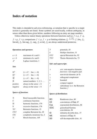
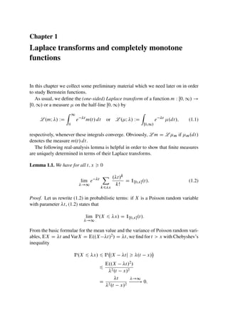
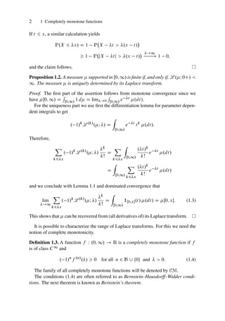
![1 Completely monotone functions 3
The version given below appeared for the first time in [34] and independently
in [287]. Subsequent proofs were given in [98] and [86]. The theorem may be also
considered as an example of the general integral representation of points in a convex
cone by means of its extremal elements. See Theorem 4.8 and [69] for an elementary
exposition. The following short and elegant proof is taken from [212].
Theorem 1.4 (Bernstein). Let f W .0; 1/ ! R be a completely monotone function.
Then it is the Laplace transform of a unique measure on Œ0; 1/, i.e. for all 0,
f ./ D L .I / D
Z
Œ0;1/
e t
.dt/:
Conversely, whenever L .I / 1 for every 0, 7! L .I / is a completely
monotone function.
Proof. Assume first that f .0C/ D 1 and f .C1/ D 0. Let 0. For any a 0
and any n 2 N, we see by Taylor’s formula
f ./ D
n 1
X
kD0
f .k/.a/
kŠ
. a/k
C
Z
a
f .n/.s/
.n 1/Š
. s/n 1
ds
D
n 1
X
kD0
. 1/kf .k/.a/
kŠ
.a /k
C
Z a
. 1/nf .n/.s/
.n 1/Š
.s /n 1
ds: (1.5)
If a , then by the assumption all terms are non-negative. Let a ! 1. Then
lim
a!1
Z a
. 1/nf .n/.s/
.n 1/Š
.s /n 1
ds D
Z 1
. 1/nf .n/.s/
.n 1/Š
.s /n 1
ds
6 f ./:
This implies that the sum in (1.5) converges for every n 2 N as a ! 1. Thus, every
term converges as a ! 1 to a non-negative limit. For n 0 let
n./ D lim
a!1
. 1/nf .n/.a/
nŠ
.a /n
:
This limit does not depend on 0. Indeed, for 0,
n./ D lim
a!1
. 1/nf .n/.a/
nŠ
.a /n
D lim
a!1
. 1/nf .n/.a/
nŠ
.a /n .a /n
.a /n
D n./:](https://image.slidesharecdn.com/740668-250517230336-4df0d2aa/85/Bernstein-Functions-Theory-And-Applications-Rene-Schilling-20-320.jpg)
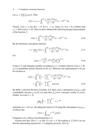
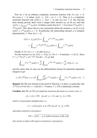
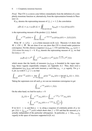
![1 Completely monotone functions 7
The seemingly innocuous closure assertion of Corollary 1.6 actually says that on
the set CM the notions of pointwise convergence, locally uniform convergence, and
even convergence in the space C1.0; 1/ coincide. This situation reminds remotely
of the famous Montel’s theorem from the theory of analytic functions, see e.g. Beren-
stein and Gay [21, Theorem 2.2.8].
Corollary 1.7. Let .fn/n2N be a sequence of completely monotone functions such
that the limit limn!1 fn./ D f ./ exists for all 2 .0; 1/. Then f 2 CM and
limn!1 f
.k/
n ./ D f .k/./ for all k 2 N [ ¹0º locally uniformly in 2 .0; 1/.
Proof. From Corollary 1.6 we know already that f 2 CM. Moreover, we have seen
that the representing measures n of fn converge vaguely in Œ0; 1/ to the representing
measure of f . By the differentiation lemma for parameter dependent integrals we
infer
f .k/
n ./ D . 1/k
Z
Œ0;1/
tk
e t
n.dt/
n!1
! . 1/k
Z
Œ0;1/
tk
e t
.dt/ D f .k/
./;
since t 7! tke t is a function that vanishes at infinity, cf. (A.3) in Appendix A.1.
Finally, assume that j j 6 ı for some ı 0. Using the elementary estimate
je t e t j 6 j j t e .^/t , ; ; t 0, we conclude that for ; and all
0
ˇ
ˇf .k/
n ./ f .k/
n ./
ˇ
ˇ 6
Z
.0;1/
ˇ
ˇe t
e t
ˇ
ˇ tk
n.dt/
6 ı
Z
.0;1/
e .^/t
tkC1
n.dt/
D ı
ˇ
ˇf .kC1/
n . ^ /
ˇ
ˇ:
Using that limn!1 f
.kC1/
n . ^ / D f .kC1/. ^ /, we find for sufficiently large
values of n ˇ
ˇf .k/
n ./ f .k/
n ./
ˇ
ˇ 6 2ı sup
ˇ
ˇf .kC1/
. /
ˇ
ˇ:
This proves that the functions f
.k/
n are uniformly equicontinuous on Œ; 1/. There-
fore, the convergence limn!1 f
.k/
n ./ D f .k/./ is locally uniform on Œ; 1/ for
every 0. Since 0 was arbitrary, we are done.
Remark 1.8. The representation formula for completely monotone functions given in
Theorem 1.4 has an interesting interpretation in connection with the Kreı̆n–Milman
theorem and the Choquet representation theorem. The set
®
f 2 CM W f .0C/ D 1
¯](https://image.slidesharecdn.com/740668-250517230336-4df0d2aa/85/Bernstein-Functions-Theory-And-Applications-Rene-Schilling-24-320.jpg)
![8 1 Completely monotone functions
is a basis of the convex cone CMb, and its extremal points are given by
et ./ D e t
; 0 6 t 1; and e1./ D 1¹0º./;
see Phelps [234, Lemma 2.2], Lax [199, p. 139] or the proof of Theorem 4.8. These
extremal points are formally defined for 2 Œ0; 1/ with the understanding that
e1j.0;1/ 0. Therefore, the representation formula from Theorem 1.4 becomes
a Choquet representation of the elements of CMb,
Z
Œ0;1/
e t
.dt/ D
Z
Œ0;1
e t
.dt/; 2 .0; 1/:
In particular, the functions
et j.0;1/
are prime examples of completely monotone functions. Theorem 1.4 and Corol-
lary 1.6 tell us that every f 2 CM can be written as an ‘integral mixture’ of the
extremal CM-functions ¹et j.0;1/ W 0 6 t 1º.
It was pointed out in [256] that the conditions (1.4) are redundant. The following
proof of this fact is from [109].
Proposition 1.9. Let f W .0; 1/ ! R be a C1 function such that f 0, f 0 6 0
and . 1/nf .n/ 0 for infinitely many n 2 N. Then f is a completely monotone
function.
Proof. Let n 2 be such that . 1/nf .n/./ 0 for all 0. By Taylor’s formula,
for every a 0
f ./ D
n 1
X
kD0
f .k/.a/
kŠ
. a/k
C . 1/n
Z
a
. 1/nf .n/.s/
.n 1/Š
. s/n 1
ds:
If n is even
f ./
n 1
X
kD0
f .k/.a/
kŠ
. a/k
;
while for n odd
f ./ 6
n 1
X
kD0
f .k/.a/
kŠ
. a/k
:
Dividing by . a/n 1, letting ! 1, and by using that f ./ is non-increasing,
we arrive at f .n 1/.a/ 6 0 in case n is even, and f .n 1/.a/ 0 in case n is odd.
Thus, . 1/n 1f .n 1/.a/ 0. It follows inductively that . 1/kf .k/.a/ 0 for all
k D 0; 1; : : : ; n. Since n can be taken arbitrarily large, and a 0 is arbitrary, the
proof is completed.](https://image.slidesharecdn.com/740668-250517230336-4df0d2aa/85/Bernstein-Functions-Theory-And-Applications-Rene-Schilling-25-320.jpg)
![1 Completely monotone functions 9
Comments 1.10. Standard references for Laplace transforms include D. V. Widder’s monographs [289,
290] and Doetsch’s treatise [80]. For a modern point of view we refer to Berg and Forst [29] and Berg,
Christensen and Ressel [28]. The most comprehensive tables of Laplace transforms are the Bateman
manuscript project [91] and the tables by Prudnikov, Brychkov and Marichev [239].
The concept of complete monotonicity seems to go back to S. Bernstein [32] who studied functions
on an interval I R having positive derivatives of all orders. If I D . 1; 0 this is, up to a change of
sign in the variable, complete monotonicity. In later papers, Bernstein refers to functions enjoying this
property as absolument monotone, see the appendix première note, [33, pt. IV, p. 190], and in [34] he
states and proves Theorem 1.4 for functions on the negative half-axis.
Following Schur (probably [258]), Hausdorff [123, p. 80] calls a sequence .n/n2N total monoton—
the literal translation totally monotone is only rarely used, e.g. in Hardy [118]; the modern terminology
is completely monotone and appears for the first time in [287]—if all iterated differences . 1/kkn
are non-negative where n WD nC1 n. Hausdorff focusses in [123, 124] on the moment prob-
lem: the n are of the form
R
.0;1 tn .dt/ for some measure on .0; 1 if, and only if, the sequence
.n/n2N[¹0º is total monoton; moreover, he introduces the moment function WD
R
.0;1 t .dt/
which he also calls total monoton. A simple change of variables .0; 1 3 t e u; u 2 Œ0; 1/, shows
that D
R
Œ0;1/ e u Q
.du/ for some suitable image measure Q
of . This means that every moment
sequence gives rise to a unique completely monotone function. The converse is much easier since
Z
Œ0;1/
e u
Q
.du/ D
1
X
nD0
. 1/nn
nŠ
Z
Œ0;1/
un
Q
.du/:
Many historical comments can be found in the second part, pp. 29–44, of Ky Fan’s memoir [94]. For
an up-to-date survey we recommend the scholarly commentary by Chatterji [63] written for Hausdorff’s
collected works [125]. More general higher monotonicity properties of the type that f satisfies (1.4) only
for n 2 ¹0; 1; : : : ; N º, N 2 N [ ¹0º, were used by Hartman [119] in connection with Bessel functions
and solutions of second-order ordinary differential equations. Further applications of CM and related
functions to ordinary differential equations can be found, e.g. in Lorch et al. [204] and Mahajan and
Ross [207], see also the study by van Haeringen [282] and the references given there. The connection
between integral equations and CM are extensively covered in the monographs by Gripenberg et al. [112]
and Prüss [240].
A by-product of the proof of Proposition 1.2 is an example of a so-called real inversion formula for
Laplace transforms. Formula (1.3) is due to Dubourdieu [86] and Feller [98], see also Pollard [238] and
Widder [289, p. 295] and [290, Chapter 6]. Our presentation follows Feller [100, VII.6].
The proof of Bernstein’s theorem, Theorem 1.4, also contains a real inversion formula for the Laplace
transform: (1.8) coincides with the operator Lk;y.f .// of Widder [290, p. 140] and, up to a constant,
also [289, p. 288]. Since the proof of Theorem 1.4 relies on a compactness argument using subsequences,
the weak limit fnk
.t/ dt ! .dt/ might depend on the actual subsequence .nk/k2N. If we combine
this argument with Proposition 1.2, we get at once that all subsequences lead to the same and that,
therefore, the weak limit of the full sequence fn.t/ dt ! .dt/ exists.
The representation (1.6) was also obtained in [87] in the following way: because of f .C1/ D
0 we can write f ./ D
R 1
. 1/f 0.t1/ dt1. Since f 0 is again completely monotone and satisfies
f 0.C1/ D 0, the same argument proves that f ./ D
R 1
R 1
t1
f 00.t2/ dt2 dt1. By induction, for
every n 2 N,
f ./ D
Z 1
Z 1
t1
Z 1
tn 1
. 1/n
f .n/
.tn/ dtn dt2 dt1:
The representation (1.6) follows by using Fubini’s theorem and reversing the order of integration. The
rest of the proof is now similar to our presentation.
It is possible to avoid the compactness argument in Theorem 1.4 and to give an ‘intuitionistic’ proof,
see van Herk [284, Theorem 33] who did this for the class S (denoted by ¹F º in [284]) of Stieltjes
functions which is contained in CM; his arguments work also for CM.](https://image.slidesharecdn.com/740668-250517230336-4df0d2aa/85/Bernstein-Functions-Theory-And-Applications-Rene-Schilling-26-320.jpg)
![10 1 Completely monotone functions
A proof of Theorem 1.4 using Choquet’s theorem or the Kreı̆n–Milman theorem can be found in
Kendall [170], Meyer [214] or Choquet [69, 68]. A modern textbook version is contained in Lax [199,
Chapter 14.3, p. 138], Phelps [234, Chapter 2], Becker [19] and also in Theorem 4.8 below. Gneiting’s
short note [109] contains an example showing that one cannot weaken the Bernstein–Hausdorff–Widder
conditions beyond what is stated in Proposition 1.9.
There is a deep geometric connection between completely monotone functions and the problem when
a metric space can be embedded into a Hilbert space H. The basic result is due to Schoenberg [255]
who proves that a function f on Œ0; 1/ with f .0/ D f .0C/ is completely monotone if, and only if,
7! f .jj2/, 2 Rd , is positive definite for all dimensions d 0, cf. Theorem 12.14.](https://image.slidesharecdn.com/740668-250517230336-4df0d2aa/85/Bernstein-Functions-Theory-And-Applications-Rene-Schilling-27-320.jpg)
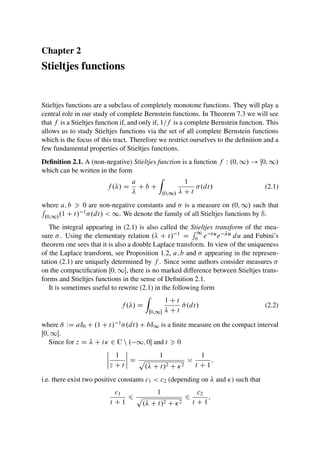
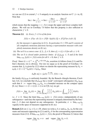
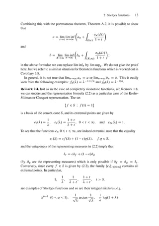
![14 2 Stieltjes functions
which we obtain if we choose 1
sin.˛/ t˛ 1 dt, 1.0;1/.t/ dt
2
p
t
or 1
t 1.1;1/.t/ dt as
the representing measures .dt/ in (2.1).
The closure assertion of Theorem 2.2 says, in particular, that on the set S the notions
of pointwise convergence, locally uniform convergence, and even convergence in the
space C1 coincide, cf. also Corollary 1.7.
Comments 2.5. The Stieltjes transform appears for the first time in the famous papers [268, 269] where
T. J. Stieltjes investigates continued fractions in order to solve what we nowadays call the Stieltjes
Moment Problem. For an appreciation of Stieltjes’ achievements see the contributions of W. van Assche
and W. A. J. Luxemburg in [270, Vol. 1].
The name Stieltjes transform for the integral (2.1) was coined by Doetsch [79] and, independently,
Widder [288]. Earlier works, e.g. Perron [231], call
R
. C t/ 1 .dt/ Stieltjes integral (German: Stielt-
jes’sches Integral) but terminology has changed since then. Sometimes the name Hilbert–Hankel trans-
form is also used in the literature, cf. Lax [199, p. 185]. A systematic account of the properties of the
Stieltjes transform is given in [289, Chapter VIII].
Stieltjes functions are discussed by van Herk [284] as class ¹F º in the wider context of moment
and complex interpolation problems, see also the Comments 6.12, 7.16. Van Herk uses the integral
representation Z
Œ0;1
1
1 s C sz
.ds/
which can be transformed by the change of variables t D s 1 1 2 Œ0; 1 for s 2 Œ0; 1 into the form
(2.2); N
.dt/ and .ds/ are image measures under this transformation. Van Herk only observes that his
class ¹F º contains S, but comparing [284, Theorem 7.50] with our result (7.2) in Chapter 7 below shows
that ¹F º D S.
In his paper [135] F. Hirsch introduces Stieltjes transforms into potential theory and identifies S as
a convex cone operating on the abstract potentials, i.e. the densely defined inverses of the infinitesi-
mal generators of C0-semigroups. Hirsch establishes several properties of the cone S, which are later
extended by Berg [22, 23]. A presentation of this material from a potential theoretic point of view is
contained in the monograph [29, Chapter 14] by Berg and Forst, the connections to the moment problem
are surveyed in [25].
Theorem 2.2 appears in Hirsch [135, Proposition 1], but with a different proof.
In contrast to completely monotone functions, S is not closed under multiplication. This follows
easily since the (necessarily unique) representing measure of 7! . C a/ 1. C b/ 1, 0 a b,
is .b t/ 1ıa.dt/ C .a t/ 1ıb.dt/ which is a signed measure. We will see in Proposition 7.10
that S is still logarithmically convex. It is known, see Hirschman and Widder [140, VII 7.4], that the
product
R
.0;1/. C t/ 11.dt/
R
.0;1/. C t/ 12.dt/ is of the form
R
.0;1/. C t/ 2 .dt/ for some
measure . The latter integral is often called a generalized Stieltjes transform. The following related
result is due to Srivastava and Tuan [264]: if f 2 Lp.0; 1/ and g 2 Lq.0; 1/ with 1 p; q 1 and
r 1 D p 1 C q 1 1, then there is some h 2 Lr .0; 1/ such that L 2.f I /L 2.gI / D L 2.hI /
holds. Since
h.t/ D f .t/ p.v.
Z 1
0
g.u/
u t
du C g.t/ p.v.
Z 1
0
f .u/
u t
du;
h will, in general, change its sign even if f; g are non-negative.](https://image.slidesharecdn.com/740668-250517230336-4df0d2aa/85/Bernstein-Functions-Theory-And-Applications-Rene-Schilling-31-320.jpg)
![Chapter 3
Bernstein functions
We are now ready to introduce the class of Bernstein functions which are closely
related to completely monotone functions. The notion of Bernstein functions goes
back to the potential theory school of A. Beurling and J. Deny and was subsequently
adopted by C. Berg and G. Forst [29], see also [25]. S. Bochner [50] calls them
completely monotone mappings (as opposed to completely monotone functions) and
probabilists still prefer the term Laplace exponents, see e.g. Bertoin [36, 38]; the
reason will become clear from Theorem 5.2.
Definition 3.1. A function f W .0; 1/ ! R is a Bernstein function if f is of class
C1, f ./ 0 for all 0 and
. 1/n 1
f .n/
./ 0 for all n 2 N and 0: (3.1)
The set of all Bernstein functions will be denoted by BF.
It is easy to see from the definition that, for example, the fractional powers 7! ˛,
are Bernstein functions if, and only if, 0 6 ˛ 6 1.
The key to the next theorem is the observation that a non-negative C1-function
f W .0; 1/ ! R is a Bernstein function if, and only if, f 0 is a completely monotone
function.
Theorem 3.2. A function f W .0; 1/ ! R is a Bernstein function if, and only if, it
admits the representation
f ./ D a C b C
Z
.0;1/
.1 e t
/ .dt/; (3.2)
where a; b 0 and is a measure on .0; 1/ satisfying
R
.0;1/.1 ^ t/ .dt/ 1.
In particular, the triplet .a; b; / determines f uniquely and vice versa.
Remark 3.3. (i) The representing measure and the characteristic triplet .a; b; /
from (3.2) are often called the Lévy measure and the Lévy triplet of the Bernstein
function f . The formula (3.2) is called the Lévy–Khintchine representation of f .](https://image.slidesharecdn.com/740668-250517230336-4df0d2aa/85/Bernstein-Functions-Theory-And-Applications-Rene-Schilling-32-320.jpg)
![16 3 Bernstein functions
(ii) A useful variant of the representation formula (3.2) can be obtained by an appli-
cation of Fubini’s theorem. Since
Z
.0;1/
.1 e t
/ .dt/ D
Z
.0;1/
Z
.0;t/
e s
ds .dt/
D
Z 1
0
Z
.s;1/
e s
.dt/ ds
D
Z 1
0
e s
.s; 1/ ds
we get that any Bernstein function can be written in the form
f ./ D a C b C
Z
.0;1/
e s
M.s/ ds (3.3)
where M.s/ D M.s/ D .s; 1/ is a non-increasing, right-continuous function.
Integration by parts and the observation that
R 1
0 se s ds D 2 and
R 1
0 e s ds D
1 yield
f ./ D 2
Z
.0;1/
e s
k.s/ ds D 2
L .kI / (3.4)
with k.s/ D as C b C
R s
0 M.t/ dt, compare with Theorem 6.2(iii). Note that k is
positive, non-decreasing and concave.
(iii) The integrability condition
R
.0;1/.1 ^ t/ .dt/ 1 ensures that the integral
in (3.2) converges for some, hence all, 0. This is immediately seen from the
convexity inequalities
t
1 C t
6 1 e t
6 1 ^ t 6 2
t
1 C t
; t 0
and the fact that for 1 [respectively for 0 1] and all t 0
1 ^ t 6 1 ^ .t/ 6 .1 ^ t/
respectively .1 ^ t/ 6 1 ^ .t/ 6 1 ^ t
:
(iv) A useful consequence of the above estimate and the representation formula (3.2)
are the following formulae to calculate the coefficients a and b:
a D f .0C/ and b D lim
!1
f ./
:
The first formula is obvious while the second follows from (3.2) and the dominated
convergence theorem: 1 e t 6 1 ^ .t/ and lim!1.1 e t /= D 0.](https://image.slidesharecdn.com/740668-250517230336-4df0d2aa/85/Bernstein-Functions-Theory-And-Applications-Rene-Schilling-33-320.jpg)
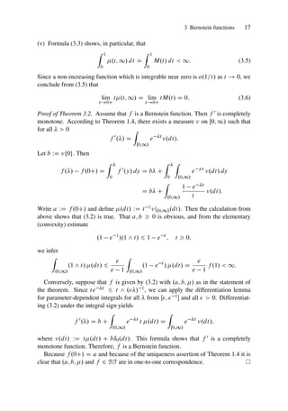
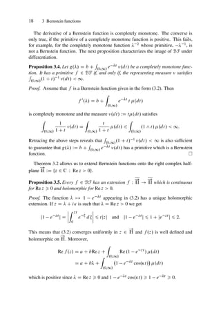
![3 Bernstein functions 19
Continuity up to the boundary follows from the estimate
jf .z/ f .w/j 6 bjz wj C
Z
.0;1/
je wt
e zt
j .dt/
6 bjz wj C
Z
.0;1/
2 ^ .tjw zj/ .dt/
for all z; w 2
!
H and the dominated convergence theorem.
The following structural characterization comes from Bochner [50, pp. 83–84]
where Bernstein functions are called completely monotone mappings.
Theorem 3.6. Let f be a positive function on .0; 1/. Then the following assertions
are equivalent.
(i) f 2 BF.
(ii) g ı f 2 CM for every g 2 CM.
(iii) e uf 2 CM for every u 0.
Proof. The proof relies on the following formula for the n-th derivative of the com-
position h D g ı f due to Faa di Bruno [93], see also [111, formula 0.430]:
h.n/
./ D
X
.m;i1;:::;i`/
nŠ
i1Š i`Š
g.m/
f ./
`
Y
j D1
f .j/./
jŠ
!ij
(3.7)
where
P
.m;i1;:::;i`/ stands for summation over all ` 2 N and all i1; : : : ; i` 2 N [ ¹0º
such that
P`
jD1 j ij D n and
P`
jD1 ij D m.
(i))(ii) Assume that f 2 BF and g 2 CM. Then h./ D g.f .// 0. Multiply
formula (3.7) by . 1/n and observe that n D mC
P`
jD1.j 1/ij . The assumptions
f 2 BF and g 2 CM guarantee that each term in the formula multiplied by . 1/n is
non-negative. This proves that h D g ı f 2 CM.
(ii))(iii) This follows from the fact that g./ WD gu./ WD e u, u 0, is
completely monotone.
(iii))(i) The series e uf ./ D
P1
j D0
. 1/j uj
jŠ Œf ./j and all of its formal deriva-
tives (w.r.t. ) converge uniformly, so we can calculate dn
dn e uf ./ by termwise dif-
ferentiation. Since e uf is completely monotone, we get
0 6 . 1/n dn
dn
e uf ./
D
1
X
j D1
uj
jŠ
. 1/nCj dn
dn
f ./
j
:
Dividing by u 0 and letting u ! 0 we see
0 6 . 1/nC1 dn
dn
f ./:](https://image.slidesharecdn.com/740668-250517230336-4df0d2aa/85/Bernstein-Functions-Theory-And-Applications-Rene-Schilling-36-320.jpg)
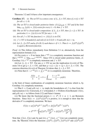
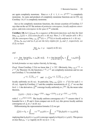
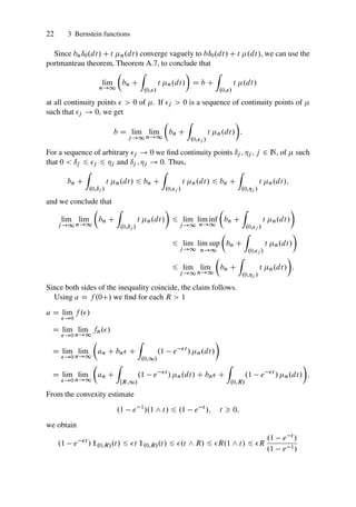
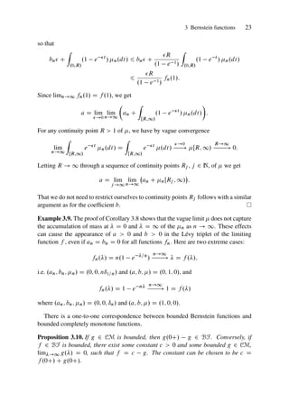
![24 3 Bernstein functions
Proof. Assume that g D L 2 CM is bounded. This means that .0; 1/ D
g.0C/ D sup0 g./ 1. Hence, f ./ WD g.0C/ g./ D
R
.0;1/.1
e t / .dt/ is a bounded Bernstein function.
Conversely, if f 2 BF is bounded, f ./ D a C
R
.0;1/.1 e t /.dt/ for some
bounded measure , cf. Corollary 3.7. Thus f ./ D c g./ where g./ D L .I /
is completely monotone, lim!1 g./ D 0 and c D a C .0; 1/ D f .0C/ C
g.0C/ 0.
Remark 3.11. Just as in the case of completely monotone functions, see Remark 1.8,
we can understand the representation formula (3.2) as a particular case of a Kreı̆n–
Milman or Choquet representation. The set
²
f 2 BF W
Z
.0;1/
f ./e
d D 1
³
is a basis of the convex cone BF, and its extremal points are given by
e0./ D ; et ./ D
1 C t
t
.1 e t
/; 0 t 1; and e1./ D 1;
see Harzallah [122] or [251, Satz 2.9]. These functions are, of course, examples
and building blocks for all Bernstein functions: every f 2 BF can be written as an
‘integral mixture’ of the above extremal Bernstein functions. If we choose .dt/ D
˛=€.1 ˛/ t 1 ˛ dt, ˛ 2 .0; 1/, .dt/ D e t , or .dt/ D t 1e t we see that the
functions
˛
.0 ˛ 1/; or
1 C
or log.1 C /
are Bernstein functions.
Comments 3.12. The name Bernstein function is not universally accepted in the literature. It originated
in the potential theory school of A. Beurling and J. Deny, but the name as such does not appear in Beur-
ling’s or Deny’s papers. The earliest mentioning of Bernstein functions as well as a nice presentation of
their properties is Faraut [95]. Bochner [50] calls Bernstein functions completely monotone mappings
but this notion was only adopted in the 1959 paper by Woll [292]. Other names include inner transfor-
mations of CM (Schoenberg [255]), Laplace or subordinator exponents (Bertoin [36, 38]), log-Laplace
transforms or positive functions with completely monotone derivative (Feller [100]).
Bochner pointed out the importance of Bernstein functions already in [49] and [50]; he defines them
through the equivalent property (ii) of Theorem 3.6. The equivalence of (i) and (ii) in Theorem 3.6
is already present in Schoenberg’s paper [255, Theorem 8]; Schoenberg defines Bernstein functions
as primitives of completely monotone functions and calls them inner transformations (of completely
monotone functions); his notation is T for the class BF. Many properties as well as higher-dimensional
analogues are given in [50, Chapter 4]. In particular, Theorems 3.2 and 3.6 can already be found there.
An up-to-date account is given in the books by Berg and Forst [29, Chapter 9] (based on [95]) and Berg,
Christensen and Ressel [28]. One can understand (3.2) as a Lévy–Khintchine formula for the semigroup
.Œ0; 1/; C/. This justifies the name Lévy measure and Lévy triplet for and .a; b; /, respectively; this
point of view is taken in [28]. The representation (3.4) is taken from Prüss [240, Chapter I.4.1] who
calls the functions k.s/ (of the type needed in (3.4), i.e. positive, non-decreasing and concave) creep
functions. The characterization of Bernstein functions using Choquet’s representation is due to Harzallah
[120, 121, 122], a slightly different version is given in [251], reprinted in [157, Theorem 3.9.20].](https://image.slidesharecdn.com/740668-250517230336-4df0d2aa/85/Bernstein-Functions-Theory-And-Applications-Rene-Schilling-41-320.jpg)
![Chapter 4
Positive and negative definite functions
Positive and negative definite functions appear naturally in connection with Fourier
analysis and potential theory. In this chapter we will see that (bounded) completely
monotone functions correspond to continuous positive definite functions on .0; 1/
and that Bernstein functions correspond to continuous negative definite functions on
the half-line. On Rd the notion of positive definiteness is familiar to most readers; for
our purposes it is useful to adopt a more abstract point of view which includes both
settings, Rd and the half-line Œ0; 1/.
An abelian semigroup with involution .S; C; / is a nonempty set equipped with a
commutative and associative addition C, a zero element 0 and a mapping W S ! S
called involution, satisfying
(a) .s C t/ D s C t for all s; t 2 S;
(b) .s/ D s for all s 2 S.
We are mainly interested in the semigroups .Œ0; 1/; C/ and .Rd ; C/ where ‘C’ is
the usual addition; the respective involutions are the identity mapping s 7! s in Œ0; 1/
and the reflection at the origin 7! in Rd . We will only develop those parts of
the theory that allow us to characterize CM and BF as positive and negative definite
functions on the half-line. Good expositions of the general case are the monographs
by Berg, Christensen, Ressel [28] (for semigroups) and Berg, Forst [29] (for abelian
groups).
Definition 4.1. A function f W S ! C is positive definite if
n
X
j;kD1
f .sj C s
k / cj N
ck 0 (4.1)
holds for all n 2 N, all s1; : : : ; sn 2 S and all c1; : : : ; cn 2 C.
We need some simple properties of positive definite functions.
Lemma 4.2. Let f W S ! C be positive definite. Then f .s C s/ 0 for all s 2 S
and f is hermitian, i.e. f .s/ D f .s/. In particular, f .0/ 0.
Lemma 4.2 shows also that positive definite functions on Œ0; 1/ are non-negative:
f 0.](https://image.slidesharecdn.com/740668-250517230336-4df0d2aa/85/Bernstein-Functions-Theory-And-Applications-Rene-Schilling-42-320.jpg)
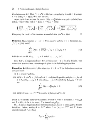
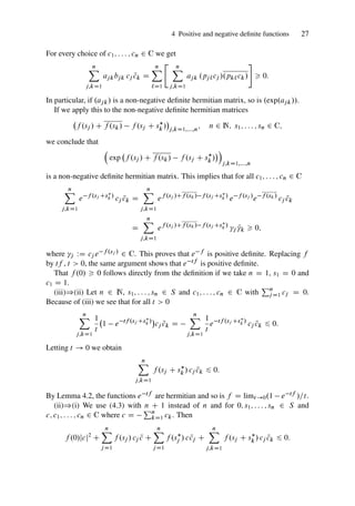
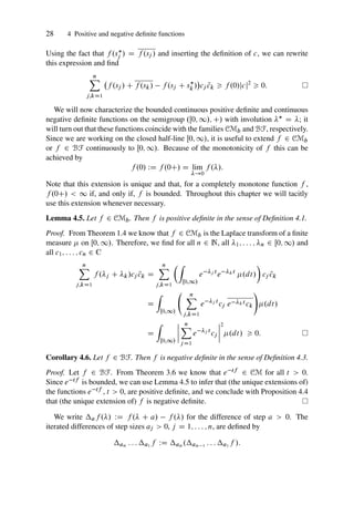
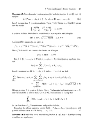
![30 4 Positive and negative definite functions
(i) f 0 and . 1/nan : : : a1 f 0 for all n 2 N and a1; : : : ; an 0.
(ii) There exists a non-negative measure on Œ0; 1/ such that
f ./ D
Z
Œ0;1/
e t
.dt/:
(iii) f is infinitely often differentiable and . 1/nf .n/ 0 for all n 2 N.
Proof. (i))(ii) Denote by B.0; 1/ the real-valued Borel measurable functions on
.0; 1/. Then
C WD
®
f 2 B.0; 1/ W f 0 and . 1/n
an : : : a1 f 0
for all n 2 N and a1; : : : ; an 0
¯
is a convex cone. If we equip B.0; 1/ with the topology of pointwise convergence,
its topological dual separates points. Since every f 2 C is non-increasing and non-
negative, the limit f .0C/ exists, and f is bounded if, and only if, f .0C/ 1.
For f 2 C the second differences are non-negative; in particular aaf 0
which we may rewrite as
f ./ C f . C 2a/ 2f . C a/; ; a 0:
This means that f is mid-point convex. Since f jŒc;d is finite on every compact
interval Œc; d .0; 1/, we conclude that f j.c;d/ is continuous for all d c 0,
i.e. f is continuous, see for example Donoghue [83, pp. 12–13].
Define K WD ¹f 2 C W f .0C/ D 1º; this is a closed subset of C. Since it is
contained in the set Œ0; 1.0;1/ B.0; 1/ which is, by Tychonov’s theorem, compact
under pointwise convergence, it is also compact. Moreover, K is a basis of the cone
Cb since for every f 2 Cb the normalized function f=f .0C/ 2 K.
Now the Kreı̆n–Milman theorem applies and shows that K is the closed convex hull
of its extreme points. For f 2 Cb we write
f ./ D f . C a/ C f ./ f . C a/
D f . C a/ C . 1/af ./:
It follows directly from the definition of the set C that f . C a/ and af are again
in Cb. Thus, if f 2 K is extremal, both functions must be multiples of f . In particu-
lar,
f . C a/ D c.a/f ./; 0; a 0:
Letting ! 0 we see that f .a/ D c.a/.
Since f .0C/ D 1 and since f is continuous, all solutions of the functional equation
f . C a/ D f .a/f ./ are of the form f ./ D et ./ D e t where t 2 Œ0; 1/. This
means that the extreme points of K are contained in the set ¹et W t 0º. Since K is](https://image.slidesharecdn.com/740668-250517230336-4df0d2aa/85/Bernstein-Functions-Theory-And-Applications-Rene-Schilling-47-320.jpg)
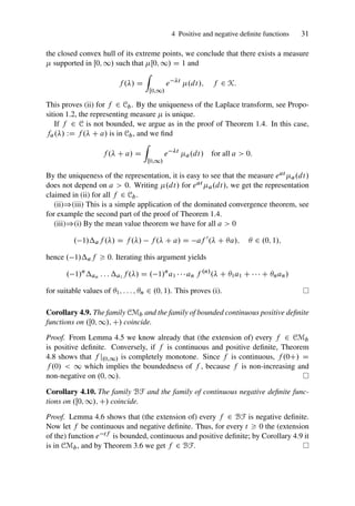
![32 4 Positive and negative definite functions
Let us briefly review the notion of positive and negative definiteness on the group
.Rd ; C/. Our standard reference is the monograph [29] by Berg and Forst.
On Rd the involution is given by D , 2 Rd . This means that f is positive
definite (in the sense of Bochner) if
n
X
j;kD1
f .j k/ cj N
ck 0; (4.6)
and negative definite (in the sense of Schoenberg) if
n
X
j;kD1
f .j / C f .k/ f .j k/
cj N
ck 0 (4.7)
hold for all n 2 N, 1; : : : ; n 2 Rd and c1; : : : ; cn 2 C.
The Rd -analogue of Lemma 4.5 and Corollary 4.9 is known as Bochner’s theorem.
Theorem 4.11 (Bochner). A function W Rd ! C is continuous and positive definite
if, and only if, it is the Fourier transform of a finite measure on Rd ,
./ D b
./ D
Z
Rd
eix
.dx/; 2 Rd
:
The measure is uniquely determined by , and vice versa.
Lemma 4.6 and Corollary 4.10 become on Rd the Lévy–Khintchine representation.
Theorem 4.12 (Lévy; Khintchine). A function W Rd ! C is continuous and nega-
tive definite if, and only if, there exist a number ˛ 0, a vector ˇ 2 Rd , a symmetric
and positive semi-definite matrix Q 2 Rdd and a measure on Rd n ¹0º satisfying
R
y¤0.1 ^ jyj2/ .dy/ 1 such that
./ D ˛ C iˇ C
1
2
Q C
Z
y¤0
1 eiy
C
i y
1 C jyj2
.dy/: (4.8)
The quadruple .˛; ˇ; Q; / is uniquely determined by , and vice versa.
Comments 4.13. Standard references for positive and negative definite functions are the monographs
[28] by Berg, Christensen and Ressel and [29] by Berg and Forst. For a more probabilistic presentation
we refer to Dellacherie and Meyer [77, Chapter X].
The natural notion of positive and negative definiteness of a (finite-dimensional) matrix was extended
to functions by Mercer [213]. A function (or kernel) of positive type is a continuous and symmetric
function W Œa; b Œa; b ! R satisfying
Z b
a
Z b
a
.s; t/ .s/.t/ ds dt 0 for all 2 CŒa; b:
This condition is originally due to Hilbert [132] who refers to it as Definitheit (definiteness). It is
shown in [213] that this is equivalent to saying that for all n 2 N and s1; : : : ; sn 2 R the matrices](https://image.slidesharecdn.com/740668-250517230336-4df0d2aa/85/Bernstein-Functions-Theory-And-Applications-Rene-Schilling-49-320.jpg)
![4 Positive and negative definite functions 33
..sj ; sk// are non-negative definite hermitian, which is in accordance with Definition 4.1. Mercer
says that is of negative type if is of positive type. Note that this does not match our definition
of negative definiteness which appears first in Schoenberg [255] and, independently, in Beurling [41];
the name negative definite was first used by Beurling [42] in connection with bounded negative definite
functions—these are all of the form c f where f is positive definite and c is a constant c f .0/, see
e.g. [29, 7.11–7.13]—while Definition 4.3 seems to appear first in Beurling and Deny [43].
The notion of a positive definite function was introduced by Mathias [210] and further developed
by Bochner [48, Chapter IV.20] culminating in his characterization of all positive definite functions,
Theorem 4.11.
Note that, in general, a negative definite function is not the negative of a positive definite function—
and vice versa. In order to avoid any confusion, many authors nowadays use ‘positive definite (in the
sense of Bochner)’ and ‘negative definite (in the sense of Schoenberg)’.
The abstract framework of positive (and negative) definiteness on semigroups is due to Ressel [243]
and Berg, Christensen and Ressel [27]. Ressel observes that positive definiteness (in a semigroup sense)
establishes the connection between two seemingly different topics: Fourier transforms and Bochner’s
theorem on the one hand and, on the other, Laplace transforms, completely monotone functions and
Bernstein’s theorem. Note that in the case of abelian groups there are always two choices for involutions:
s WD s, which is natural for groups, and s D s which is natural for semigroups. Each leads to a
different notion of positive and negative definiteness.
The proof of Proposition 4.4 is adapted from [29, Chapter II.7] and [28, Chapters 4.3, 4.4]; for The-
orems 4.7 and 4.8 we used Dellacherie–Meyer [77, X.73 and X.75] as well as Lax [199, Chapter 14.3].
The best references for continuous negative definite functions on Rd are [29, Chapter II] and [77, Chap-
ter X].](https://image.slidesharecdn.com/740668-250517230336-4df0d2aa/85/Bernstein-Functions-Theory-And-Applications-Rene-Schilling-50-320.jpg)
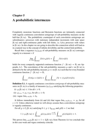
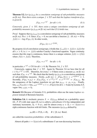
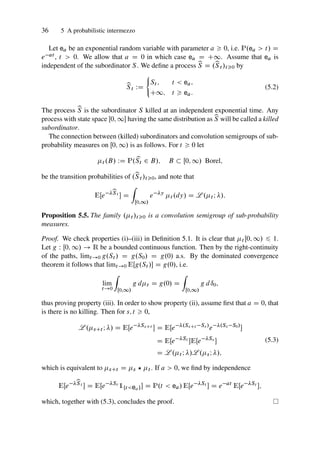
![5 A probabilistic intermezzo 37
The converse of Proposition 5.5 is also true: given a convolution semigroup .t /t0
of sub-probability measures on Œ0; 1/, there exists a killed subordinator .St /t0 on a
probability space .; F; P/ such that t D P.St 2 / for all t 0. A proof of this
fact can be found in [36].
Let us rewrite (5.1) as
EŒe b
St
D L .t I / D e tf ./
:
Recall that f 2 BF has the representation
f ./ D a C b C
Z
.0;1/
.1 e t
/ .dt/:
It is clear from the proof of Theorem 5.2 that a D f .0C/ 0 if, and only if,
t Œ0; 1/ 1 for all t 0; in this case, the associated stochastic process has a.s.
finite lifetime. This is why a is usually called the killing term of the Laplace expo-
nent f .
Let .t /t0 be a convolution semigroup of sub-probability measures on Œ0; 1/
and let f be the corresponding Bernstein function. Then the completely monotone
function g./ WD L .1I / D e f ./ has the property that for every t 0, gt is
again completely monotone. This follows easily from
gt
./ D e tf ./
D L .t I /:
From the probabilistic point of view, this means that St is an infinitely divisible ran-
dom variable. To be more precise St D
Pn
j D1.Sjt=n S.j 1/t=n/ for every n 2 N.
The random variables .Sjt=n S.j 1/t=n/16j 6n are independent and identically dis-
tributed. Hence t D ?n
t=n
is the n-fold convolution. This motivates the following
definition.
Definition 5.6. A completely monotone function g is said to be infinitely divisible if
for every t 0 the function gt is again completely monotone.
If g is infinitely divisible and g.0C/ 6 1, the sub-probability measure on Œ0; 1/
satisfying L D g is said to be an infinitely divisible distribution; we write 2 ID.
The discussion preceding the definition shows that if f 2 BF, then g WD e f is
completely monotone and infinitely divisible. Moreover, g.0C/ 6 1. This is already
one direction of the next result.
Lemma 5.7. Suppose that g W .0; 1/ ! .0; 1/. Then the following statements are
equivalent.
(i) g 2 CM, g is infinitely divisible and g.0C/ 6 1.
(ii) g D e f where f 2 BF.](https://image.slidesharecdn.com/740668-250517230336-4df0d2aa/85/Bernstein-Functions-Theory-And-Applications-Rene-Schilling-54-320.jpg)