BARRERA-THESIS-2015

THE INFLUENCE OF DAM RELEASES ON MICROBIAL AND
PHYSIOCHEMICAL PARAMETERS IN THE ALLUVIAL AQUIFER OF A
REGULATED RIVER
A Thesis
by
CHRISTINA SUZETTE BARRERA
Submitted to the Office of Graduate and Professional Studies of
Texas A&M University
in partial fulfillment of the requirements for the degree of
MASTER OF SCIENCE
Chair of Committee, Terry Gentry
Co-Chair of Committee, Peter Knappett
Committee Members, Jacqueline Aitkenhead-Peterson
Paul DeLaune
Raghupathy Karthikeyan
Allen Berthold
Head of Department, David Baltensperger
May 2015
Major Subject: Soil Science
Copyright 2015 Christina Suzette Barrera

ii
ABSTRACT
Elevated fecal indicator bacteria in river systems is a continuing concern in
Texas and throughout the United States. It has been discovered that bacterial
concentrations in surface waters can increase drastically during elevated flow events.
These events can be induced by natural, or anthropologic causes. An example of the
latter is releases of large amounts of water from dams. These large releases of water to a
river system may also influence the state of the surrounding alluvial groundwater. The
aim of this study was to better understand changes in bacterial concentrations in the
saturated alluvium approximately 19.3 kilometers downstream of the Tom Miller Dam,
following regular, dam releases every 24 hours. A transect of 4 groundwater wells, at
distances 1.5 to 6 meters from the river, was installed perpendicular to the bank of the
Colorado River near Austin, TX. The wells were sampled every 4 hours over a 24-hour
period. Field measurements were taken for temperature, electrical conductivity, pH and
dissolved oxygen (DO). Laboratory tests were used to determine concentrations of total
coliforms, fecal coliforms, E. coli, PO4-P, NO3-N, dissolved organic carbon (DOC), and
total nitrogen (TN). Results indicated that the dam release had little impact on bacterial
concentrations of the surrounding alluvium with increases detected only in the well
closest to the river at peak water levels. During the time in which these samples were
collected, the river system was under relatively low-flow conditions with the regular
dam release only raising the water level about 0.06 m (0.2 ft) during sampling.
Therefore, following sampling, the wells were fitted with pressure transducers to

iii
quantify lateral hydraulic gradients as a function of river level. Lateral hydraulic
gradients confirmed the small dam releases, currently occurring upstream of the site,
were not large enough to reverse the natural groundwater flow direction away from the
river, consistent with the microbial and chemical results.

iv
DEDICATION
I dedicate this thesis to my grandparents, Mr. and Mrs. Arnoldo Barrera Sr. and
Mr. and Mrs. Carlos Tamayo. You all always taught me to appreciate everything that I
have, to pursue my dreams and, no matter what, to work hard in order to reach my fullest
potential. I love you all more than I could ever hope to express.

v
ACKNOWLEDGMENTS
I would like to thank my committee chair, Dr. Terry Gentry, my committee co-
chair, Dr. Peter Knappett, and my committee members, Dr. Aitkenhead-Peterson, Dr.
DeLaune, and Dr. Karthikeyan, for their guidance and support throughout the course of
this research. Further thanks are extended to Carla Young for her assistance during
sampling and laboratory work and for her understanding during stressful moments in the
project.
Thanks also go to my friends, colleagues and the department faculty and staff for
making my time at Texas A&M University a great experience. I also want to extend my
gratitude to Dr. Anderson at the Center for Environmental Research and the Austin
Youth River Watch, whom graciously allowed me to use their headquarters during
sampling events.
Finally, I would like to thank my mother, father and brother for their unending
encouragement, love and support.

vi
TABLE OF CONTENTS
Page
ABSTRACT .............................................................................................................. ii
DEDICATION........................................................................................................... iv
ACKNOWLEDGMENTS.......................................................................................... v
TABLE OF CONTENTS........................................................................................... vi
LIST OF FIGURES ................................................................................................... viii
1. INTRODUCTION ............................................................................................... 1
2. LITERATURE REVIEW..................................................................................... 3
2.1. Dam releases.................................................................................................3
2.2. Stream and groundwater exchange ................................................................ 5
2.3. Filtration properties of the riverbank ............................................................. 7
2.4. Escherichia coli ............................................................................................ 8
2.5. Cryptosporidium and Enterovirus.................................................................. 9
2.6. Water chemistry............................................................................................ 10
3. MATERIALS AND METHODS.......................................................................... 13
3.1. Monitoring wells........................................................................................... 13
3.2. Pumps ........................................................................................................... 16
3.3. Sampling....................................................................................................... 17
3.3.1. Bacterial and chemical collection........................................................ 19
3.3.2. Cryptosporidium and Enterovirus collection ....................................... 20
3.3.3. Field parameters ................................................................................. 20
3.3.4. Pressure transducer data collection...................................................... 21
3.4. Laboratory analysis ....................................................................................... 22
3.4.1. Bacterial analysis................................................................................ 22
3.4.2. Chemical analysis ............................................................................... 22
3.4.2.1. Ammonium nitrogen .................................................................. 22
3.4.2.2. Nitrate nitrogen.......................................................................... 23
3.4.2.3. Phosphate phosphorus................................................................ 23
3.4.2.4. Dissolved organic carbon and total nitrogen.............................. 23
3.4.3. Cryptosporidium and Enterovirus analysis .......................................... 24
3.5. Statistical analysis ......................................................................................... 28
4. RESULTS AND DISCUSSION........................................................................... 29
4.1. Water levels and hydraulic gradient............................................................... 29
4.2. Field measurements....................................................................................... 34

vii
4.3. Water chemistry............................................................................................ 38
4.4. Bacterial concentrations ................................................................................ 42
4.5. Statistical analysis ......................................................................................... 45
4.6. Cryptosporidium and Enterovirus.................................................................. 46
5. CONCLUSIONS.................................................................................................. 47
REFERENCES.......................................................................................................... 50

viii
LIST OF FIGURES
FIGURE Page
2.1. The hyporheic zone allows for water exchange from the surface
stream into underlying groundwater and adjacent alluvial aquifer ......................6
3.1. Well transect located along the Colorado River at Hornsby Bend in
Austin, TX. TCEQ Station ID #21411 ...............................................................14
3.2. Hornsby Bend well transect showing the Colorado River in the
background and groundwater wells 05, 10, 15, and 20. .....................................15
3.3. Map of Austin area, showing the locations of Austin Lake and Tom
Miller Dam (blue), Lady Bird Lake and Longhorn Dam (yellow)
and Hornsby Bend research well transect (red star, N30°13’56.8”,
W97°39’12.6”). ................................................................................................16
3.4. Colorado River flowing at approximately 10,000 cfs following a
storm event in October 2013..............................................................................19
4.1. Graph shows the average rainfall in Austin, Texas and the change in
the height of the Colorado River at Hwy 183, prior to, during, and
after the October 2-3 sampling event, highlighted in green.................................29
4.2. Graph shows the average rainfall in Austin, Texas and the change in
river height at Hwy 183 prior to, during, and after the June 8-9 and
16-17 sampling events, highlighted in green. .....................................................30
4.3. Profile plot of the water table beginning at the river (00) and reaching
to Well 20 at Hornsby Bend over a 9 hour period, when the river
pulses from its lowest to its highest point, on October 8-9, 2013.. ......................31
4.4. Hydraulic gradient change graphs that correspond to increase in the
water table. ........................................................................................................32
4.5. Flow velocity graphs of the groundwater in the alluvial aquifer
adjacent to the Colorado River. .........................................................................33

ix
4.6. Water temperature of samples collected during October 2-3 (A), June
(B), and June 16-17 (C) sampling events (TCEQ Station ID
#21411). ............................................................................................................35
4.7. pH of samples collected during October 2-3 (A), June 8-9 (B), and
June 16-17 (C) sampling events (TCEQ Station ID #21411). .............................36
4.8. Electrical conductivity readings of samples collected during October
2-3 (A), June 8-9 (B), and June 16-17 (C) sampling events (TCEQ
Station ID #21411). ...........................................................................................37
4.9. Dissolved oxygen reading of samples collected during October 2-3
(A), June 8-9 (B), and June 16-17 (C) sampling events (TCEQ
Station ID #21411). ...........................................................................................38
4.10. Nitrate-nitrogen concentrations for samples collected during the
October 2-3 (A), June 8-9 (B), and June 16-17 (C) sampling events
(TCEQ Station ID #21411). ...............................................................................39
4.11. Total nitrogen concentrations from samples collected during the
(TCEQ Station ID #21411). ...............................................................................40
4.12. Ammonium-nitrogen concentrations from the samples collected
during the October 2-3 (A), June 8-9 (B), and June 16-17 (C)
sampling events (TCEQ Station ID #21411). .....................................................40
4.13. Phosphate-phosphorus concentrations from samples collected during
the October 2-3 (A), June 8-9 (B), and June 16-17 (C) sampling
events (TCEQ Station ID #21411). ....................................................................41
4.14. Dissolved organic carbon concentrations in samples collected during
4.15. Escherichia coli concentrations in water samples collected during

x
4.16. Fecal coliform concentrations in water samples collected during the
(TCEQ Station ID #21411). ...............................................................................44
4.17. Total coliform concentrations in water samples collected during the
(TCEQ Station ID #21411). ...............................................................................45
4.18. Statistical results for the E. coli predictors in river samples.................................45

1
1. INTRODUCTION
In many locations throughout the world, clean drinking water is not accessible to
communities that are in desperate need of it. In such cases, shallow drinking water wells
are installed in close proximity to surface water in the hopes that these groundwater
wells are less contaminated than the nearby surface water. Natural filtration processes
that occur in the adjacent saturated alluvium tend to purify the surface water of many
contaminants (Tufenkji et al., 2002). Natural exchange between surface and groundwater
fluctuates in direction and magnitude depending on the hydraulic gradient of the area. In
an area where water table and river levels are similar, low flow river conditions may
cause the river to receive groundwater. This is known as a gaining stream. During high
river stage, however, the hydraulic gradient may be reversed and water would be forced
into the surrounding alluvium.
The river associated with this project is the Colorado River. This river is the
longest to be completely within the borders of the state of Texas. Its headwaters begin
around Lamesa, TX, and the river travels approximately 1,387.25 km (862 miles) until it
empties into Matagorda Bay near Houston, TX. There are two man-made lakes along the
river that affect this project. The first is Austin Lake, created due to the construction of
Tom Miller Dam, and the second is Lady Bird Lake, created due to the construction of
Longhorn Dam (Figure 3.3). Tom Miller Dam was constructed primarily for flood
control and hydroelectricity production purposes. This facility provides electricity to the
city of Austin, especially during high use summer months. The dam is also used to

2
supplement the natural downstream flow in the river, provide water to the residents
living along the river and supply the coastal estuaries with freshwater. Water is released
from Austin Lake once every 24 hours causing a pulse in river flow that travels
downstream until it reaches Lady Bird Lake. If the lake levels at Lady Bird lake are low,
this water refills the lake. However, if the water levels at Lady Bird Lake are normal, the
additional water passes through the spillway gates at Longhorn Dam and continues
downstream.
This pulse in river flow and its effects on the breadth of the hyporheic zone of the
river was studied by Sawyer et al. (2002). They found that the river stage, at the time,
increased up to 2.8 m (9.2 ft) over a 24 hour period. Additionally, the river pulses were
reversing the hydraulic gradient of the area up to 30 m (98.4 ft) into the river bank. In
addition to the findings from that project, in 2010, the U.S. Environmental Protection
Agency classified 8 km (5 mi.) of river, 5.8 km (3.6 mi.) upstream of Hornsby Bend
(Figure 3.3.), as impaired due to bacterial contamination (USEPA, 2015). These two
veracities could have a profound impact on the alluvial groundwater of the Colorado
river system if the change in hydraulic gradient meant that impaired surface water was
interacting with the alluvial groundwater.
The main objective of this research was to measure the effect of a rising and
falling river stage along the Colorado River in Texas, over 24 hour periods, in order to
determine if concentrations of microbial fecal indicators and pathogens in the river
affected the microbial concentrations of the alluvial groundwater.

3
2. LITERTURE REVIEW
Water is an undeniably important resource for continuation of life on this planet.
The state of water quality all over the world is of growing concern. All topics addressed
in this review are key components to the purpose of this thesis. Without these
components, an accurate understanding of the influence of dam releases on the state of
alluvial groundwater would be impossible. The topics covered include the impact of
hydroelectric dam releases on the down-stream hydrology, stream and groundwater
exchange through riverbank filtration, utilization of physiochemical water parameters as
water tracers, and the measurement of microbial water quality indicators. Despite the
array in which these topics are presented, this review focus’ on their application toward
understanding the impacts that dam releases may have on the microbial and
physiochemical parameters in the alluvial aquifer of a regulated river.
2.1. Dam Releases
All water, whether in liquid, solid, or gaseous form, make up the hydrosphere of
the earth (Shiklomanov, 2000), which totals 1.386 x 106
km3
. Of this hydrosphere only
2.5% is freshwater, and of this freshwater, 68.7% is frozen, 29.9% is classified as
groundwater and only about 0.26% is available as surface water in lakes, rivers and
streams (Carpenter et al., 2011). Currently, the upper limit of available fresh water has
not been exceeded by human water usage, however, that is based on the global average.
There are approximately 2.4 billion people living in areas that are considered highly
water stressed (Oki and Kanae, 2006), and water management is crucial in these places.

4
The human solution to this problem is to install dams within large river systems to
impound water in places that are in short supply during most of the year. Of the major
river systems on the earth, dams affect over half (Nilsson et al., 2005). These effects are
seen in the both the upstream and downstream portions of the river, and range from
inundation of the floodplain upstream to temperature and water chemistry alterations
downstream (Nilsson et al., 2005; World Commission on Dams, 2000).
Downstream effects are especially predominant below hydroelectric dams due to
the large scheduled releases of water that power the turbines. These large releases cause
a rise in the river stage that has the potential to force water into the surrounding
riverbank and change the hydraulic gradient of the area. Then, if normal conditions favor
a gaining stream, as the water recedes, the gradient changes back so that groundwater
flows toward the river (Curry et al., 1994; Singh, 2004). This changes drainage water
chemistry at specific locations along the river. Smart et al. (2001) found evidence that
the geochemical characteristics of the riparian area had a significant influence on the
chemical composition of the receding water. River stage increases from anthropogenic
influences are often quite different from river stage changes brought about by natural
events; such as storms, and so may cause changes not seen during natural occurrences.
Temperature is a physical water characteristic that is often measured to be different
upstream and downstream of a dam. Cooler waters, associated with the hypolimnion of
the water body upstream of the dam, are released and alter the temperatures and oxygen
concentrations of downstream environments (Hancook, 2002). Hill et al. (2000) found

5
that microbial respiration, of the sediment near a stream containing cooler water,
decreased, due to the negative impact on mesophilic microorganisms.
2.2. Stream and groundwater exchange
Natural river and stream systems are not consistent in their discharge and,
instead, change from season to season and even from day to day (Cardenas, 2009).
Under normal flow conditions, a stream system is considered to be either a gaining or a
losing stream. When the groundwater table is higher than the surface of the stream,
water will flow toward the stream, replenishing the river with what is known as base
flow. Conversely, if the groundwater table is lower than the surface of the stream then
water will flow toward the groundwater table (Sawyer et al., 2009). Surrounding these
stream systems is an area of surface water and groundwater exchange known as the
hyporheic zone, which literally means “under flow” (Boulton, 2000) and is named so
since it is the area in which surface water infiltrates the alluvial aquifers and underlying
groundwater (Figure 2.1).

6
Figure 2.1. The hyporheic zone allows for water exchange from the surface stream into
underlying groundwater and adjacent alluvial aquifers.
Hyporheic zone exchange is influenced by pressure and hydraulic gradients of
the area (Cardenas, 2009). For rivers regulated by dams, changes in water height are
consistent, as opposed to natural systems that are subject to seasonal flooding. In cases
of rivers that are regulated by hydroelectric dams, water stage changes in the river follow
an undulating pattern as water is released regularly for the production of electricity.
During peak flow, under release schedules, it is possible that the hydraulic gradient
between the surface water and the groundwater reverses from its natural state. Another
way to explain this occurrence is through the Gill-Lung Model (Sawyer et al., 2009).
The model illustrates that during base-flow the hyporheic zone exchange of water is

7
shallow relative to the river, however, during regulated flow, such as under dam release
conditions, the water exchange in the hyporheic zone is much deeper and dynamic.
Due to the influence of surface water, pressure gradients and directional flow
changes, there are substantial amounts of water mixing occurring within the hyporheic
zone and extending, sometimes, into groundwater. This mixing of these separate bodies
of water establishes an environment that is suitable for high levels of biogeochemical
cycling and bacterial growth. This dynamic nature of the hyporheic zone and its relative
inaccessibility which makes physical mapping and special characterization of the
aforementioned processes difficult. However, in one study, Cardenas et al. (2011)
utilized electrical resistivity imaging (ERI) to map the extent and dynamics of water
mixing and flow paths within the alluvial material along the Colorado River located in
Austin, Texas. This study found that the hyporheic zone of the area extends several
meters deep and across the entire channel bed. This size and extent would not be
possible if the Colorado River was not a regulated river. Rivers that remain at low flow
status for extended periods tend to have a shallow hyporheic zone, where surface water
is not forced into and out of the hyporheic zone but merely flows through it. Thus, it can
be hypothesized that the dam releases that result in an undulating river stage may also
affect the amount of bacteria found in the surrounding groundwater due to water being
forced downward.
2.3. Filtration properties of the riverbank
The fate of microbial organisms in soils likely depends on both biotic and abiotic
controlling factors (van Keen et al., 1997). Biotic controls include competition and the

8
production of inhibitory substances by other organisms that may affect the survival of
soil organisms. Due to this, increases in the survival rates of bacteria, such as
Escherichia coli, occur when the microbial soil community is diminished in its
complexity (van Elsas et al., 2007). Abiotic factors include mechanisms such as colloid
straining. Escherichia coli was found to become retained through straining in finer-
textured soils at a greater rate than mechanisms like physico-chemical attachment
(Bradford and Bettahar, 2005). As water moves within soils, deposition profiles for a
range of microorganisms, like bacteria, viruses and protozoa, suggest that with
increasing distance from the origin of contamination there is a decreasing rate of
deposition (Albinger et al., 1994; DeFlaun et al., 1997; Baygents et al., 1998; Simoni et
al., 1998; Bolster et al., 2000; Redman et al., 2001; Zhang et al., 2001; Bradford et al.,
2002; Li et al., 2004; Bradford and Bettahar, 2005). In combination with straining,
physico-chemical filtration aid in the removal of colloidal particles from water that
moves through the soil matrix. The surface charge of soil particles, coupled with the
charges on colloids enhance physico-chemical filtration. (Li et al., 2004).
2.4. Escherichia coli
When scientists look for the existence of pathogens in water samples, they do not
test every water sample for the presence of every known pathogen, due to the high cost
associated with such a method. In order to test many samples at a relatively low cost
they test for the presence of indicator organisms. An important characteristic of an
indicator organism is that it is able to persist in the same environment as the organism(s)
of concern. However, because of many factors, including a variation in rates of survival,

9
the lifespan of specific bacteria or viruses cannot be correlated with the presence or
absence of indicator organisms (Dorner et al., 2004; Ferguson et al., 2012). The indicator
organisms primarily used are total coliforms, fecal coliforms and E. coli. Escherichia
coli is itself a fecal coliform but is the most widely used as an indicator organism
because of its association with fecal contamination (CDC, 2009). These indicator
organisms are of bacterial origin and are easily cultured in a laboratory setting on agar
plates or through the use of Most Probable Number methods.
2.5. Cryptosporidium and Enterovirus
Cryptosporidium parvum was recognized first as an animal pathogen in 1955,
and not until 1976 was it identified as a human pathogen. C. parvum is a protozoan,
obligate parasite that multiplies within its host. It causes infections and self-limiting
diarrhea in healthy adults, but in infants, the elderly, or anyone that is
immunocompromised, it may cause fatal diarrhea. The oocysts of this species of
Cryptosporidium are very hardy and environmentally resistant, which allows them to
persist outside of their host once they are shed from the body through the fecal matter
(Szewzyk et al., 2000). The Enterovirus group encompasses a few different virus types
which include Polioviruses 1-3, Coxsackievirus A, Coxsackievirus B, Echoviruses, and
Enterovirus 68-71. All of these virus types inhabit the human alimentary tract, which
means that they are transmitted via the fecal-oral route. The spectrum of Enterovirus
disease is vast, from permanent paralysis to subclinical infection. The latter is much
more common than the occurrence of a clinically manifested disease (Melnick, 1982).

10
2.6. Water chemistry
There is a substantial link between water shortage and water quality. Water
contamination reduces the amount of usable water available and also drives up the price
of water treatment. Nonpoint pollution is considered to be the most significant source for
nitrogen, phosphorus and carbon in natural water systems (Carpenter et al., 1998).
Nitrogen is an abundant element in the environment. Natural sources to watersheds
include rock weathering, lightning and wet precipitation, N-fixation to vegetation, fecal
matter from wildlife and death and decay of vegetation and animals. Anthropogenic
sources include mineral fertilizers applied to agricultural crops and homeowner
landscapes in urban and suburban watersheds, rain out of volatilized ammonia and fecal
matter and death and decay of domestic animals. Of the nitrogen species, nitrate is an
extremely conservative molecule and is easily leached through soil toward groundwater
or washed out of the soil during rainstorms and runoff events. This will cause the
nitrogen to become unusable to plants, because it will be out of the reach of their root
systems. When that occurs the end point for this nitrogen species is usually groundwater
pools or rivers and streams (Bai et al., 2012).
Phosphorus is used as an additive to agricultural farms and private lawn and garden
soils as a fertilizer. Although, anthropogenic sources of phosphorus have almost tripled
the global mobilization of this nutrient, a small portion is made mobile due to natural
sources such as decay of dead biomass, and solubilization of soil phosphates by
microorganisms (Smil, 2000). Phosphorus is unique in its cycling because phosphorus
rarely enters a gaseous form, which confines it to the soil and water of the environment.

11
Phosphorus is the limiting nutrient in freshwater aquatic systems and any increase, no
matter how small, could cause unwanted effects. These could include increased algal
growth and decreased oxygen levels that could in turn negatively influence the
population of aquatic life. There are two forms of phosphorus is the aquatic
environment, organic and inorganic. Organic phosphorus is incorporated in plant and
animal tissues, while inorganic phosphorus, the form available for plant uptake, is not.
Both forms have the potential to be dissolved or suspended in the water column. The
concentration of phosphate in the water column, largely depends on the adsorption and
desorption properties to the surrounding sediment, as equilibrium is controlled by this
exchange of phosphate into and off of particle surfaces (Kerr et al., 2011). The same
may also be true of organic carbon within shallow groundwater.
Dissolved organic carbon (DOC) in shallow groundwater, especially
groundwater that is used as a drinking water source, has unwanted aesthetic
considerations as well as an influence on microbial growth (Wassenaar et al, 1996).
Most DOC concentrations in natural groundwater sources are between the
concentrations of < 1 mg/L to 100 mg/L (Chomycia et al 2008; Wassenaar et al, 1991
and Wassenaar et al, 1996), however, the concentrations all depend on the differences in
organic matter origin and materials that makeup the overlying aquifer soils (Chomycia et
al, 2008). High humic soils and seasonal changes in the amount of vegetative growth in
the area all contribute to a change in carbon concentrations. Groundwater with high
DOC concentrations provide significant sources of carbon for microbes (Findlay et al,
1993), such as E. coli. Studies performed by Bolster et al. (2005) and Surbeck et al.

12
(2010) showed results that E. coli thrive and even show signs of population recovery in
waters that contain high DOC and other nutrients.
Surface water and groundwater has very distinct chemical characteristics, these
characteristics allow them to be useful tools in monitoring the movement of water
between streams and alluvial aquifers.

13
3. MATERIALS AND METHODS
3.1 Monitoring wells
A transect of four wells was installed along the Colorado River in Austin, Texas
(TCEQ Station ID #21411). The well site (N30°13’56.8”, W97°39’12.6”) is located at
Hornsby Bend and the Center for Environmental Research. All wells were installed
using a Geoprobe and were installed to a depth of approximately 3 m (10 ft). They were
all screened across the entire water table and are each located 1.5 m (5 ft.) from the
previous, with the first well being installed 1.5 m from the edge of the river at the time
of installation (Figure 3.1 and 3.2).
Throughout the duration of the project, all river height data was obtained from a
USGS gauge that is located under highway 183, approximately 11.6 km (7.2 mi)
upstream of the research site (USGS 08158000 Colorado River at Austin, TX) (Figure
3.3). The elevation measurements were adjusted by applying a constant, which was
calculated by taking the difference in datum elevations (meters above sea level) from
each site and then applying that difference to all subsequent water elevation
measurements.

14
Figure 3.1. Well transect located along the Colorado River at Hornsby Bend in Austin,
TX. TCEQ Station ID #21411

15
Figure 3.2. Hornsby Bend well transect showing the Colorado River in the background
and groundwater wells 05, 10, 15, and 20.

16
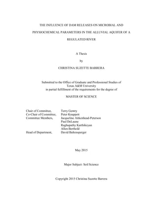
Figure 3.3. Map of Austin area, showing the locations of Austin Lake and Tom Miller
Dam (blue), Lady Bird Lake and Longhorn Dam (yellow) and Hornsby Bend research
well transect (red star, N30°13’56.8”, W97°39’12.6”) . In 2010, the section of the river
highlighted in red was classified as impaired due to bacterial contamination by
recreational standards.
3.2 Pumps
During the first round of sampling (Table 3.1), a Masterflex E/S portable
peristaltic pump (Cole-Parmer, Vernon Hills, IL) was utilized. Sampling from the
groundwater wells, during the second and third rounds of sampling, was done using four
Poseidon 12V submersible water pumps (Groundwater Essentials, Bradenton, FL); one
individual pump was used for each of the four wells in order to avoid cross-
contamination between wells. The tubing setup remained the same for all three rounds,

17
with only minor alterations in order to accommodate the pumps. The tubing used was
standard 6.35 mm (1/4 in) ID polypropylene tubing with a backflow regulator attached
to the end to prevent contamination of the well from outside sources. Before each
sampling event, the pumps and tubing system were disinfected using a 200 mg/l chlorine
solution, which was run through the pumps and tubing until 19 liters was used. The
pump and tubing was then rinsed using 40 liters of reverse osmosis water to ensure that
all residual chlorine was removed. A HACH DR 2800 spectrophotometer and TNT 867
chlorine detection kit (Hach Company, Loveland, Colorado) was used to confirm that
chlorine removal was successful. Before each sample was collected from the
groundwater wells, two entire well volumes were purged to ensure that water from the
alluvium was being sampled and not stagnant water in the well column. Samples were
collected from the river, adjacent to the well transect, using a telescoping swing sampler
(Nasco, Ft. Atkinson, WI). These surface water samples were collected from an area 3 m
from the river bank.
3.3 Sampling
There were a total of four sampling dates throughout the duration of this project
(Table 3.1). Of the four events, three were over a period of 24 hours, with one exception,
while only one was used for the purposes of Cryptosporidium and Enterovirus
collection.
Approximately a week prior to the October event, there was a significant storm
event that passed through the Austin area and caused a 1.8 m (6 ft) increase in river
stage. This sizable increase in river stage caused the Hornsby Bend well field to become

18
inundated with river water (Figure 3.4). Another storm, prior to the June 16-17 event,
caused an increase in the river stage, however, it was not significant enough to flood the
well field.
Event Date Label* Period Parameters Measured
October 2-3, 2013 A 24 hours Temperature
Electrical Conductivity
Dissolved Oxygen
Microbial
Chemical
June 8-9, 2014 B 20 hours Temperature
Dissolved Oxygen
Microbial
Chemical
June 11, 2014 M - Cryptosporidium
Enterovirus
June 16-17, 2014 C 24 hours Temperature
Dissolved Oxygen
Microbial
Chemical
Table 3.1. Shows sampling event dates and samples collected during each event.
*All labels correspond to their assigned sampling date throughout this thesis.

19
Figure 3.4. Colorado River flowing at approximately 10,000 cfs following a storm
event in October 2013.
3.3.1 Bacteria and chemical collection
All three of the 24-hour sampling rounds were scheduled to capture normal flow
conditions of the river, and were not performed unless there had been, at least, three days
between the end of the last rain event and the sampling event. Each round consisted of a
complete 24-hours of sampling, with the exception of round 2 (June 8-9) for which the
last sample was not collected due to the onset of rain in the area. Samples were collected
every 4 hours relative to the first sample collected. For every groundwater and river

20
sample, two sample bottles of water were collected. One 500 mL bottle was used for
bacterial samples that were transferred to the Lower Colorado River Authority (LCRA)
Environmental Services Laboratory, and one 125 mL, acid washed, collection bottle was
used for the collection of chemical samples which were returned to Texas A&M
University and analyzed in Dr. Aitkenhead-Peterson’s laboratory.
3.3.2 Cryptosporidium and Enterovirus collection
Sampling for Cryptosporidium and Enterovirus was performed on June 11, 2014,
which was separate from the normal sampling dates. Water samples were collected as
described for sampling events 2 and 3 above. Once well purging was completed, a total
of 10 liters from each site was pumped through an Envirochek®
HV sampling capsules
(Pall, Port Washington, NY) for Cryptosporidium and a NanoCeram®
cartridge filter
(Argonide, Sanford, FL) for Enterovirus collection. All filters were placed on ice in a
cooler and transported back to Texas A&M University for further analysis.
3.3.3. Field parameters
Field parameters, including temperature, specific conductivity, pH and dissolved
oxygen was measured at the same time that samples were taken. During the first
sampling event a YSI Professional Plus Multiparameter Handheld instrument with
Quatro Cable and respective detection probes was used (YSI Incorporated, Yellow
Springs, Ohio). However, due to equipment malfunction, pH was unable to be taken with
the YSI probe during the second sampling event. The LCRA Environmental Services lab
conducted pH measurements on all the water samples during that event. During the final
sampling event, a second YSI instrument was utilized, a YSI 556 MPS. All instruments

21
were calibrated during the morning of the scheduled sampling event, again halfway
through the sampling event, and then a final time upon the conclusion of the event to
make certain that they remained calibrated over the entire 24 hours.
3.3.4 Pressure transducer data collection
Two pressure transducers (Model 3001 Levelogger Edge, Solinst Canada Ltd.,
Georgetown, Ontario, Canada) and two TLC probes (Model 3001 LTC Junior, Solinst
Canada Ltd., Georgetown, Ontario, Canada) were installed in the shallow wells. All
probes measure temperature and pressure, whereas the TLC probes also measures
specific conductance of the water. The two TLC probes were installed closest to the river
since this zone experiences the greatest fluctuations in specific conductance due to
dilution of groundwater with river water during the high river stage (Sawyer et al.,
2009). The probes recorded temperature and pressure every 10 minutes. Pressures were
converted to water level elevation in two steps. The first step was subtracting
atmospheric pressure, which was recorded by a barologger on site (Barologger Edge,
Solinst, Georgetown, Canada). This step assumes a hydraulic efficiency of one which is
valid for shallow, unconfined aquifers (Spane, 1999; Gonthier, 2007). The second step
was to reference the transducer pressure readings to a manual water level below the top
of the well casing using a water level tape (Model 101, P7 Water Level Meter, Solinst
Canada Ltd., Georgetown, Ontario, Canada). To ensure that the calibration worked
correctly, each logger was calibrated twice; once at deployment and once after removal.
Calibrations were performed using a measured water depth, from the top of the well
casing, and compared to the measured pressure readings at the time of logger

22
deployment. The “actual water table” depth was calculated by subtracting the constant
that was measured immediately before deployment. The relative elevations of the tops of
the wells was measured using a Total Station (GTS-226, Topcon Positioning Systems,
Inc. Livermore, CA). This allowed water levels within each well to be compared across
the aquifer in meters above an arbitrary datum.
3.4 Laboratory analysis
3.4.1. Bacterial analysis
To test for the presence and number of total and fecal coliforms in the samples
provided to them, the LCRA Environmental Services Laboratory used Standard Method
9222 membrane filtration (MF). For the detection of Escherichia coli the laboratory used
Standard Method 9223 Colilert Quanti Trays by IDEXX (IDEXX Laboratories
Incorporated, Westbrook, Maine). Error bars associated with most probable number
(MPN) method were calculated using 95% confidence intervals (Hurley and Roscoe,
1983).
3.4.2. Chemical analysis
3.4.2.1. Ammonium nitrogen
Ammonium nitrogen content was determined using the United States
Environmental Protection Agency (USEPA) Method 350.1 (NH4-N USEPA Method
350.1). The method using phenate hypochlorite was further enhanced using nitroprusside
(Aitkenhead-Peterson et al., 2009).

23
3.4.2.2. Nitrate nitrogen
Nitrate nitrogen was determined using USEPA Method 353.2 (NO3-N USEPA
Method 353.2). Using this method, all samples underwent cadmium-copper reduction
(Aitkenhead-Peterson et al., 2009). Nitrate concentrations were determined by
subtracting the nitrate concentrations determined by SmartChem 200 Method 375-100E-
1 (Rev: A-03-0906) from the total organic nitrogen (NOx)-
determined by this same
method.
3.4.2.3. Phosphate phosphorus
Total orthophosphate phosphorus was found using USEPA Method 365.1 (PO4-P
USEPA Method 365.1). Ammonium molybdate and antimony potassium tartrate reacted
in an acid medium with dilute solutions of phosphorus to form an antimony-phospho-
molybdate complex. This complex was reduced to an intensely blue-colored complex by
ascorbic acid. The color, measured at 880 or 660 nm, is proportional to the phosphorus
concentration present within the sample.
3.4.2.4. Dissolved organic carbon and total nitrogen
Determination of non-purgeable organic carbon (NPOC) and total nitrogen (TN)
was done using a Shimadzu TOC-VCSH with Dual TN Module (Shimadzu Scientific
Corp. Koyoto, Japan) for NPOC/TN. NPOC, specifically, was found using 720°C
combustion catalytic oxidation/chemiluminescence method and TN was determined
using a combustion tube and oxidation catalyst which is shared with TOC analysis, and
chemiluminescence method.

24
3.4.3. Cryptosporidium and Enterovirus analysis
Prior to laboratory analysis, all sample cartridges were transported from the field
on ice, back to Texas A&M University, within 24 hours of the samples being collected.
All laboratory analysis, then, was executed within a 72 hours of that collection event. In
order to elute Cryptosporidium off of the Envirochek HV sampling capsules, USEPA
Method 1623.1 was followed. The filters were submerged in sodium hexametaphosphate
(NaHMP) solution and then agitated for five minutes at 900 rpm on a laboratory shaker.
NaHMP was removed and the filters were rinsed with reagent grade water. Elution
buffer was then added to the filter capsules and agitated for another five minutes at 900
rpm. The elution was collected in a 250 mL conical tube, and the elution process was
repeated another time to ensure all oocysts were removed from the filter. To elute
Enterovirus from NanoCeram®
cartridge filters, USEPA Method 1615 was followed.
Five hundred milliliters of 1.5% beef extract was allowed to sit for one minute. The
extract was then pushed through the filter using a peristaltic pump and collected. An
additional round of beef extract was pumped through the filter housing, allowed to sit for
fifteen minutes, and then collected in the same beaker. The pH of the collected beef
extract was adjusted to 3.5 so that the viruses would adhere to the flocculent that formed.
The samples were transferred to centrifuge tubes, and centrifuged at 2,500 g and 4°C for
15 minutes to the collect the pellet. The pellet was dissolved in 30 mL of 0.15 M sodium
phosphate (pH 9.0). The resuspended pellet was centrifuged at 4,000 x g for 10 minutes
at 4⁰C and the supernatant was retained. The sample pH was adjusted to 7, and the

25
supernatant was sterilized by using a 0.22 µm sterilizing filter. The final sample was
divided into three storage portions for later use.
The concentration methods continued with Method 1623.1 for the concentration
of Cryptosporidum oocysts by centrifuging the 250 mL conical tubes at 1,500 g for 15
minutes or until a pellet formed. All supernatant was removed until 5 mL above the
pellet so as not to lose any oocysts. The samples were transferred to microcentrifuge
tubes until the DNA extraction step; Method 1615 for Enterovirus continued with
Vivaspin-20 centrifugal concentrators. Samples were centrifuged at 3,000 g until all
samples were concentrated to 50 µl.
The final step, before analysis in a thermocycler, was to extract the nucleic acid
from all concentrated oocysts. Cryptosporidum sample extraction was performed
according to the DNeasy Blood & Tissue Kit. Initially, 200 µl of PBS and 20 µl of
proteinase K was added to each sample eluent. Following completion of that step, 200 µl
of buffer AL, without ethanol, was added to each of the samples. The samples were then
incubated at 56°C for 10 minutes, after which, 200 µl of ethanol was placed into each of
the sample tubes. All samples were transferred to DNeasy Mini spin columns and
centrifuged at 6000 g for 1 minute. The flow through was discarded and 500 µl of Buffer
AW1 was added to the spin column. The samples underwent another centrifugation
session at 6000 g for 1 minute. After the flow through was discarded again, 500 µl of
Buffer AW2 was added to the spin column and the column was centrifuged at 20,000 g
for 3 minutes. The flow through was discarded and the removable column was
transferred to a new 1.5 microfuge tube. For the final washing, 200 µl AW2 was added

26
to the DNeasy membrane and allowed to incubate for 1 minute. The final centrifugation
was done at 6,500 g for 1 minute. All samples were collected, quantified via Nanodrop
and stored at -20°C until qPCR was performed.
Extraction of Enterovirus viral RNA was achieved using a QIAamp Viral RNA
Spin Kit. Initially, 310 µl of buffer AVE was added to the tube containing carrier RNA.
Next, 67.2 µl of carrier RNA was mixed with 67.2 µl of AVL Buffer. For each of the
previously concentrated Enterovirus cell samples, 200 µl of RNA was transferred to a
1.5 mL microcentrifuge tube. Subsequently, 200 µl of the RNA carrier-AVL mixture
was also transferred to the 1.5 mL microcentrifuge tube. The tubes were vortexed for 15
seconds each to mix the solution before incubation at 56°C for 10 minutes. Following
incubation, the samples were centrifuged at 5,500 g for 5 seconds and then 200 µl of
ethanol was added to the tubes. The samples were vortexed and centrifuged again for 5
seconds. All samples were then transferred to the QIAamp Mini Spin column and
centrifuged at 6,000 g for 1 minute. The removable column was transferred to a new,
clean collection tube and 500 µl of Buffer AW1 was added. The mixture was centrifuged
again at 6,000 g for 1 minute and, after, the column was transferred to a new collection
tube. Another 500 µl of Buffer AW2 was added carefully to the column and the mixture
was centrifuged at 20,000 g for 3 minute. Column transfer to a new collection tube
occurred again and the whole tube was centrifuged at 20,000 g for 1 minute. Before the
final centrifugation step, the column was transferred to a clean RNA-free and DNA-free
collection tube, 50 µl of Buffer AE was added to the column and it was all allowed to
incubate at room temperature for 1 minute. This was followed by centrifugation at 6,000

27
g for 1 minute. The final samples were quantified by Nanodrop and stored in a -80°C
freezer until reverse transcriptase was performed.
The kit used to assay for Cryptosporidium DNA was a PCR Cryptosporidium kit
(Ceeram Tools, France). For each of the 40 samples, 20 µl of CRYPT/IPC Master Mix
was transferred to a 96 well optical plate. In the case of the control samples, 5 µl of
positive control and 5 µl of negative control was added to 20 µl of Master Mix each and
pipetted into individual wells. Five microliters of each of the regular samples were added
into individual wells, along with 20 µl of Master Mix. The solution in each well was
thoroughly mixed using a pipette and the plate was centrifuged at 3000 g for 3 minutes.
An optical cover was used to cover the plate and the plate was installed into a qPCR
thermocycler using these conditions: 50°C for 2 minutes, 95°C for 10 minutes, a cycling
step of 95°C for 15 seconds and 60°C for 1 minute for a total of 40 cycles, followed by a
4°C holding temperature.
A RT-PCR Enterovirus Test kit (Ceeram Tools, France) was used to obtain data
from the viral RNA. For all twelve samples, a master mix containing RT-PCR enzymes
was created using 19 µl of ENTERO/IPC Master Mix and 1 µl RT-PCR Enzyme Mix.
Five microliters of positive, negative, and sample aliquots were transferred to a 96 well
plate. Twenty microliters of Master Mix was then added to each well containing liquid
sample. Each of the samples were mixed thoroughly using a pipette and the plate was
centrifuged at 3,000 g for 3 minutes. An optical cover was applied to the plate and the
plate was inserted into a RT-PCR Thermocycler using these conditions: 45°C for 10

28
minutes, 95°C for 10 minutes, a cycling step of 95°C for 15 seconds and 60°C for 45
seconds for 40 cycles with a 4°C holding temperature.
3.5 Statistical analysis
Statistical analysis software (SPSS) with backwards stepwise regression
modeling was used to model the potential predictors of E.coli in water samples collected
during all three sampling events.

29
4.1. Water levels and hydraulic gradients
The pressure transducers installed in the wells showed the change in water
gradient within the subsurface of the river bank. The hydraulic gradient of the area
seemed to change with very large surges in the river, which were only brought on by
storm events. Figures 4.1 and 4.2 show the rainfall and river height changes prior to,
during and after all scheduled sampling events.
Figure 4.1. Graph shows the average rainfall in Austin, Texas and the change in the
height of the Colorado River at Hwy 183, prior to, during, and after the October 2-3
sampling event, highlighted in green.
0.00
0.20
0.40
0.60
0.80
1.00
1.20
1.40
0
1
2
3
4
5
6
7
8
9
10
RiverHeightChange(m)
Rainfall(cm)
Date
Rainfall (cm)
River Height
(m)
4. RESULTS AND DISCUSSION

30
Figure 4.2. Graph shows the average rainfall in Austin, Texas and the change in river
height at Hwy 183 prior to, during, and after the June 8-9 and 16-17 sampling events,
highlighted in green.
Figure 4.3 is a profile plot of the Hornsby Bend well transect. The plot begins at
the water’s edge (00) and reaches to Well 20. This presents the increase in water level
from the rivers lowest point, at 6:00 PM on October the 8th
, 2013 until the river reaches
peak flow at 3:00 AM on October 9th
, 2013. The information suggests that the small
positive pulse in river level has little effect on the groundwater table during the same
time span.
0.00
0.20
0.40
0.60
0.80
1.00
1.20
1.40
0
1
2
3
4
5
6
7
8
9
10
RiverHeightChange(m)
Rainfall(cm)
Date
Rainfall
(cm)
River
Height (m)

31
Figure 4.3. Profile plot of the water table beginning at the river (00) and reaching to
Well 20 at Hornsby Bend over a 9 hour period, when the river pulses from its lowest to
its highest point, on October 8-9, 2013.
The river heights shown in Fig. 4.3 were calculated by subtracting the difference
between two synoptic river level measurements at the USGS gauge site 11.6 km
upstream (Highway 183, Austin, TX) and at the well transect site to account for a
sloping river surface. As well as assuming a sloping river surface, this method is based
on the assumption that the magnitude of river pulses remain constant as they travel
downstream to Hornsby Bend. This assumption is not valid because the magnitude of
the river pulses decrease with distance downstream of a dam. Therefore the range in
surface water heights shown in Fig. 4.3 are larger than those that actually occurred on
6:00 PM
8:00 PM
10:00 PM
12:00 AM
2:00 AM
3:00 AM
123.10
123.12
123.14
123.16
123.18
123.20
123.22
00 05 10 15 20
WaterTableElevation(masl)
River and Well IDs

32
site. This gives the impression of larger hydraulic head differences between the river and
the aquifer. It is therefore more ideal that river stage and elevation be measured adjacent
to the well transect to accurately know river stage and hydraulic forcing conditions in
the riverbank aquifer.
Figure 4.4 shows the corresponding changes in hydraulic gradient during two
separate storm events following the first round of sampling in October of 2013. Any
hydraulic flow away from the river is shown in the upper graph where the line falls
below zero on the y axis. This shows that the hydraulic gradient of the area only reverses
under very large increases in the water table of the area. Suggesting that under a normal
dam release schedule, there is not enough of a shift in hydraulic gradient to force river
water into the alluvial aquifer.
Figure 4.4. Hydraulic gradient change graphs that correspond to increases in the water
table.

33
Flow velocities of the groundwater also change during times of very high flow in
the river; Figure 4.5 illustrates this change. The further the graph lines deviate from zero
on the y axis, the higher the velocity. Any movement in the positive direction shows
groundwater flow toward the river, and movement in the negative direction shows water
flow away from the river. This is in agreement with information reported in Sawyer et al
(2009), where on average, the river at this section is a gaining stream.
Figure 4.5. Flow velocity graphs of the groundwater in the alluvial aquifer adjacent to
the Colorado River.

34
During the storm event that occurred on October 31st
, 2013, the pressure
transducer that was taking readings in Well 10 was forcibly removed from the well by
storm debris and so data following that period of time was lost. However, what can be
concluded is that the flow of groundwater within the river bank is not uniform
throughout the extent of the well transect. The data shows that the groundwater has a
tendency to flow away from Well 10 and toward Well 15. Suggesting that either Well 10
is situated in a lower permeable area of the soil, or that Well 15 acted as a water sink.
4.2. Field measurements
Field measurements were collected during the time of sampling and included
water temperature, pH, conductivity, and dissolved oxygen of all samples. Figure 4.6.
show the temperature of the river and all groundwater well samples during all three of
the sampling events associated with this project. Among the three sampling events, the
highest peaks in the river height occurred between 1:00 AM and 2:00 AM. The overall
trends in river temperature fluctuation depended most heavily on the time of day, and
not on any fluctuation in the height of the river (Sawyer et al., 2009). During each of the
sampling events, the lowest water temperatures in the surface water were observed
between 9:00 PM and 9:00 AM of the 24-hr sampling period. At approximately 9:00
AM, the temperatures of the river samples began to rise gradually. The trends in
groundwater sample temperatures also followed this pattern, however, the range over
which the temperature changed was dampened when compared to river water
measurements.

35
Figure 4.6. Water temperature of samples collected during October 2-3 (A), June 8-9
(B), and June 16-17 (C) sampling events (TCEQ Station ID #21411).
With the exception of the June 8-9 sampling event (Figure 4.7), the pH increased
in the river water with increased river stage over a 24-hr period. The pH pulses in the
wells were not as drastic in their temporal variability, although they did exhibit slight
changes. During the June events, spatial variability between wells was lower than the
variability in October. This is likely due to the degree of water mixing that occurred
prior to the October sampling event. Figure 4.1. shows an elevated river stage that was
maintained for approximately a week in the later part of September 2013. This
prolonged, elevated river stage, likely reversed the natural hydraulic gradient of the river
bank enough to allow for a higher amount of stream water to enter the shallow aquifer.

36
Figure 4.7. pH of water samples collected during October 2-3 (A), June 8-9 (B), and
June 16-17 (C) sampling events (TCEQ Station ID #21411).
A much more accurate way to trace water using field measurements is by
examining the conductivity of the water. This is because the conductivity of surface
water is naturally much lower than the conductivity of groundwater in the area. This is
illustrated in Figure 4.8, where the value of the river water samples lay at an average
reading far below that of any groundwater sample. In comparison, the conductivity
values of the groundwater samples were recorded at levels at or above 1000 µs/cm, with
Well 15 as the exception during the October 2-3 sampling event. The samples pulled
form this well had an average reading of 774 µs/cm. The field parameter, pH, also show
evidence to the level of water mixing that occurred prior to the sampling events. The
October pH readings between the river and well water samples show a much smaller
difference. However, when compared to the June events, there was a much greater
distinction between the pH values of the river and those of the well water samples. This
alludes to a much higher level of water mixing in the subsurface prior to the month of
October, in comparison to the month of June when it appeared that there was a much
more distinct separation between river and groundwater.

37
Figure 4.8. Electrical conductivity of water samples collected during October 2-3 (A),
June 8-9 (B), and June 16-17 sampling events (TCEQ Station ID #21411).
Dissolved oxygen measurements in water are used as tracers and as indicators of
water quality. Any decline in oxygen concentration in the well water samples following
the initial collection was likely due to the collection itself. After the initial collection,
DO concentration remained relatively constant. Dissolved oxygen changes in the river
mimic the changes in water temperature closely, during the October sampling event. As
the temperature of the river water spiked slightly, fell and then increased gradually in the
early morning hours (Figure 4.6), the same trend was seen in the DO concentrations of
the river during the same sampling event (Figure 4.9). The relationship between water
temperature and dissolved oxygen concentration was not demonstrated as strongly
during the June sampling events. While there were small increases in the steady
undulating cycle of water temperature that occurred during the June sampling events at
1:00 AM and 2:00 AM, respectively. However, there were no observable changes in
dissolved oxygen concentration at these sampling times.

38
Figure 4.9. Dissolved oxygen concentrations in water samples collected during October
2-3 (A), June 8-9 (B), and June 16-17 (C) sampling events (TCEQ Station ID #21411).
4.3. Water chemistry
The chemical makeup of environmental waters change over time and under
different conditions, this change can be followed and recorded in order to better
understand the cycling of chemicals within the boundaries of a surface water-
groundwater interaction. Nitrate in the surface water during the month of October
averaged 6.5 mg/L, which was higher than the nitrate measured in the river during the
month of June, which was between 3.5 and 3.8 mg/L (Figure 4.10). United States EPA
(2015) has set the maximum contaminant level (MCL) for nitrate-nitrogen at 10 mg/L,
following this standard, the nitrate measured in the river during all sampling events is
within the regulatory standards. However, concentrations measured in unpolluted water
bodies are usually <4.0 mg/L. Higher nitrate levels in October were consistent with the
fact that there were larger, more intense rainstorms that occurred prior to that month,
followed by reduced base flow levels. Since nitrate is a highly water-soluble molecule,
more of it would have been washed into the river during these rainstorms and then there

39
was not enough water to dilute the dissolved molecules. This same reasoning can be
used to explain the higher levels of nitrate in the groundwater in October, also.
Figure 4.10. Nitrate-nitrogen concentrations for samples collected during the October 2-
3 (A), June 8-9 (B), and June 16-17 (C) sampling events (TCEQ Station ID #21411).
Total nitrogen concentrations (Figure 4.11) were not significantly different from
nitrate-nitrogen readings because of the low levels of other detectible forms of nitrogen
found in the natural environment. Water chemistry analysis of the ammonium-nitrogen
levels of the samples collected showed very low levels of this type of nitrogen (Figure
4.12), and thus supports the fact that nitrate-nitrogen was the most abundant form of
nitrogen in the water samples at the time of sampling.

40
Figure 4.11. Total nitrogen concentrations from samples collected during the October 2-
3 (A), June 8-9 (B), and June 16-17 (C) sampling events (TCEQ Station ID #21411).
Figure 4.12. Ammonium-nitrogen concentrations from the samples collected during the
October 2-3 (A), June 8-9 (B), and June 16-17 (C) sampling events (TCEQ Station ID
#21411).
Phosphate-phosphorus concentrations averaged around 0.1 mg/L in the
groundwater samples during all of the sampling events (Figures 4.13). The
concentrations in the river, like the river level, pulsed over a 24-hr period. However,
phosphate-phosphorus concentrations appeared to become reduced during times of
heightened flow in the river, and increased as the river level began to decline. This
occurred during all three of the sampling events.

41
Figure 4.13. Phosphate-phosphorus concentrations from samples collected during the
#21411).
Of all the chemical components of an environmental water system, dissolved
organic carbon (DOC) can give the best indication as to where the run-off of the area is
originating from, especially if the land use of the surrounding area is known (Gron et al,
1996). The height of the river, in relation to the DOC concentration in the river, did not
appear to have an appreciable effect. According to Wassenaar et al. (1991), common
DOC concentrations are on the order of 5 – 100 mg/L. The month of October results
showed levels that are expected in the alluvial groundwater of a river system, however,
the June sampling events showed concentrations that were much higher (Figure 4.14).
Since there was not as much water movement in and out of the alluvial transect during
the month of June, in comparison to the level predicted in October, the DOC content of
the groundwater was uninfluenced for an extended amount of time. If runoff from the
area transported large quantities of carbon into the subsurface from the surrounding area,
without continued runoff events the levels of DOC measured in the samples are not so
surprising.

42
Figure 4.14. Dissolved organic carbon concentrations in samples collected during the
#21411).
4.4 Bacterial concentrations
As mentioned in the methods section of this thesis, the LCRA Environmental
Laboratory used the Colilert method for bacterial detection. The Colilert method is an
enzyme substrate method. The method is able to detect a single, viable organism in a
sample and it suppresses noncoliform bacteria that also may be present within the
sample. It is also capable of specifically identifying E. coli cells that are present.
During all sampling rounds, E. coli concentrations in the river mirrored the rise
and fall of the river height. Peak concentrations of the bacteria occurred shortly after the
peak river height and then decreased over time (Figure 4.15). Overall, E. coli
concentrations were generally low, with the exception of two sampling periods during
the first round of sampling. During the 5:00 PM and 9:00 PM collection on October 3rd
,
E. coli concentrations rose to 416 MPN/100mL and 260 MPN/100mL, respectively.
During sampling rounds 2 and 3, E. coli levels never rose above 67 MPN/100mL. E. coli
concentrations in the groundwater remained lower than concentrations measured in the
river all three sampling trips.

43
Figure 4.15. Escherichia coli concentrations in water samples collected during the
October 2-3 (A), June 8-9 (B), and June 16-17 sampling events (TCEQ Station ID
#21411). Error bars represent the upper and lower 95th
percentile limits of uncertainty
for the data collected by IDEXX Colilert Quanti Trays.
Fecal coliform concentrations, like E. coli levels, remained lower in the
groundwater than concentrations found in the river, except for a single collection point
during round 2 where Well 10 had a slightly higher concentration (16 CFU/100 mL)
than the concentration measured in the river (10 CFU/100mL) (Figure 4.16). Fecal
coliform concentrations in the river peaked slightly after the peak in river height during
all three of the sampling events. When comparing sampling event results to one another,
the third round of sampling yielded concentrations in the groundwater that were
consistently near 1 CFU/100mL, which is lower than concentrations measured during
the previous two events.

44
Figure 4.16. Fecal coliform concentrations in water samples collected during the October
Concentrations of total coliforms in river samples, like E. coli and fecal coliform
concentrations, increased as the height of the river increased, during all three sampling
events (Figures 4.17). While concentrations of fecal coliforms, generally, remained
lower than concentrations measured in river samples, there was an exception in Well 05
during the second sampling event. Well 05 concentrations followed the increasing trend
seen in river samples, and only showed signs of decreasing during the 5:00 PM
collection, however, immediately increased again. Noticeably lower concentrations (<15
CFU/100 mL) during rounds 2 and 3, were measured in the groundwater when compared
to concentrations measured during round 1. Overall, there were no consistent trends in
change for total coliforms in the groundwater samples.

45
Figure 4.17. Total coliform concentrations in water samples collected during the October
4.5 Statistical analysis
River water samples were the only samples that were analyzed with any
confidence. Two separate models were run, with the only difference being the inclusion
of the parameter river stage. Despite the difference, both models reported the same
Standard Error of the Estimate. Results showed that water chemistry was the only
predictor of E. coli concentrations in the water samples (Figure 4.18).
Figure 4.18. Statistical results for the E. coli predictors in river water samples.

46
These results were surprising considering that the measured E. coli
concentrations obtained from IDEXX plate counts indicate that concentrations were
affected by river pulses over 24 hours. An explanation for this could lie in the fact that
while bacterial concentrations did increase with river stage increases, they were delayed
approximately 4 to 5 hours. This lag in bacterial increase, which was not considered for
in the model, most likely affected the results.
4.6 Cryptosporidium and Enterovirus
None of the samples collected and analyzed tested positive for the presence of
either Cryptosporidium or Enterovirus. These results were most likely due to the
extremely low concentration of these pathogens in the water system as evidenced by low
levels of E. coli and other fecal indicator microorganisms.

47
5. CONCLUSIONS
In contrast to the river samples, where most chemical and microbial parameters
fluctuated with river stage, there were no congruent fluctuations in those parameters in
groundwater samples. This is likely due to the low magnitude river stage fluctuations
caused by the low intensity of dam releases. Sawyer et al. (2009) found daily changes in
the river level, at an adjacent site on the river, impacted water-table fluctuations 30 m
into the surrounding aquifer and resulted in a hyporheic zone that extended
approximately 1-5 m into the riparian aquifer. However, daily dam releases to the river
were much larger during their study, producing changes in river levels of 2.5 m as
compared to 0.15 m during this study.
With the exception of two samples, river E. coli levels were below regulatory
limits (126 MPN/100 ml). This is consistent with data collected from February 2006
until February 2014, at a nearby site (TCEQ Station 12469) for which only 4 out of 48
samples exceeded 126 MPN/100 ml. Interestingly, E. coli levels rose with river height
and peaked shortly after the river level began to fall. An explanation for this is that rising
river levels collected additional E. coli from the surrounding riparian area and washed
them into the river as the water receded. The results from the Cryptosporidium and
Enterovirus tests found no evidence of these pathogens in the water system.
All the field parameters measured were found to be in agreement with the results
previously found by Sawyer et al. (2009). Temperature cycles are congruent with normal
diurnal river water temperature patterns. Conductivity was found to be lower in the river

48
water samples and increase in samples with increasing distance from the river. Dissolved
oxygen concentrations and pH of samples both showed strong evidence to support the
difference in the level of water mixing that occurred between sampling months. The
similarity between DO and pH values in in surface water and groundwater in October
suggests mixing of surface and groundwater occurred at a much higher rate in October in
comparison to the month of June. The results for these two field measurements in June
show a much more prominent separation between river water and groundwater
measurements.
Other water chemistry parameters also suggested evidence of higher degrees of
water mixing during the month of October, especially the organic carbon concentrations.
Whereas dissolved organic carbon concentrations were low in groundwater in October
and similar to river water, during June they were abnormally high (between 105 – 125
mg/L) (Strohmeier et al., 2013). This was likely due to an accumulation of organic
carbon from run-off events and no influx of river water to dilute the added carbon. The
low flow events in the river during the month of June also, may have, contributed to the
higher concentrations, since there was less water to dilute the added organic carbon.
Overall, the low levels of pathogens and bacterial indicator organisms coupled
with weak evidence of the mixing of river and surface water when compared to levels
seen historically, suggest that it is unlikely that the alluvial groundwater was adversely
impacted by surface water contaminants under the current dam release conditions.
Nevertheless, there is a possibility that if the dam release schedule was ever to return to

49
historical levels, the risk of pathogen infiltration into the alluvial aquifer would possibly
increase.

50
REFERENCES
Aitkenhead-Peterson, J.A., Steele, M.K., Nahar, N., and Santhy, K. (2009), Dissolved
organic carbon and nitrogen in urban and rural watersheds of south-central
Texas: land use and land management influences. Biochemistry-US. 96: 119-
129.
Albinger, O, Biesemeyer, B.K, Arnold, R.G, and Logan, B.E. (1994), Effect of bacterial
heterogeneity on adhesion t uniform collectors by monoclonal populations.
FEMS Microbiol. Lett. 124(3): 321-326.
Bai, J, Ye, X, Zhi, Y, Gao, H, Huang, L, Xiao, R, and Shao, H. (2012), Nitrate-nitrogen
transport in horizontal soil columns of the Yellow River Delta Wetland, China.
Clean-Soil Air Water. 40(10): 1106-1110.
Baygents, J.C, Glynn Jr., J.R, Albinger, O, Biesemeyer, B.K, Ogden, K.L, and Arnold,
R.G. (1998), Variations of surface charge density on monoclonal populations:
Implications for transport through porous media. Environ. Sci. Technol. 32:
1596-1603.
Bolster, C.H, Mills, A.L, Hornberger, G.M, and Herman, J.S. (1999), Spatial distribution
of deposited bacteria following miscible displacement experiments in intact
cores. Water Resour. Res. 35: 1797-1807.
Bolster, C.H, Mills, A.L, Hornberger, G, and Herman, J. (2000), Effect of intra-
population variability on the long-distance transport of bacteria. Ground Water.
38(3): 370-375.
Boulton A. (2000), River ecosystem health down under: Assessing ecological condition
in riverine groundwater zones in Australia. Ecosyst. Health. 6(2):108-118.
Bradford, S.A, and Bettahar, S.R. (2005), Straining, attachment, and detachment of
Cryptosporidium oocysts in saturated porous media. J. Environ. Qual. 34: 469-
478.
Bradford, S.A, Simunek, J, and Walker, S.L. (2006), Transport and straining of E. coli
O157:H7 in saturated porous media. Water Resour. Res. 42: W12S12

51
Bradford, S.A, Yates, S.R, Bettahar, M, and Simunek, J. (2002), Physical factors
affecting the transport and fate of colloids in saturated porous media. Water
Resour. Res. 38(12): 1327.
Cardenas, M. B. (2009), Stream-aquifer interactions and hyporheic exchange in gaining
and losing sinuous streams. Water Resour. Res. 45: 1-13.
Cardenas, M.B, and Markowski, M. (2011), Geoelectrical Imaging and Hyporheic
Exchange and Mixing of River Water and Groundwater in a Large Regulated
River. Environ. Sci. Technol. 45: 1407-1411.
Carpenter, S.R, Caraco, N.F, Correll, D.L, Howarth, R.W, Sharpley, A.N, and Smith,
V.H. (1998), Nonpoint pollution of surface waters with phosphorus and nitrogen.
Ecol. Appl. 8(3): 559-568.
Carpenter, S.R, Stanley, E.H, and Zanden, M.J.V. (2011), State of the World’s
Freshwater Ecosystems: Physical, Chemical, and Biological Changes. Annu.
Rev. Env. Resour. 36: 75-99.
Centers for Disease Control (CDC) and Prevention. (2009). Public Water Systems:
Water Quality and Testing. Online.
Chomycia, J.C., Hernes, P.J., Harter, T., and Bergamanschi, B.A. (2008), Land
management impacts on dairy-derived dissolved organic carbon in groundwater.
J. Environ. Qual. 37: 333-343.
Curry, R.A, Gehrels, J, Noakes D.L.G, Swainson, R. (1994), Effects of river flow
fluctuations on groundwater discharge through brook trout, Salvelinus fontinalis,
spawning and incubation habitats. Hydrobiologia. 277: 121-134.
DeFlaun, M.F, Murray, C.J, Holben, M, Scheibe, T, Mills, A, Ginn, T, Griffin, T, Majer,
E, and Wilson, J.L. (1997), Preliminary observations on bacterial transport in a
coastal plain aquifer. FEMS Microbiol. Rev. 20(3-4): 473-487.

52
Dorner, S.M, Huck, P.M, Slawson, R.M, Gaulin, T, and Anderson, W.B. (2004),
Assessing levels of pathogenic contamination in a heavily impacted river used as
a drinking-water source. J. Toxicol. Environ. Health A. 67: 1813-1823.
Ferguson, A., Layton, A. A., Mailloux, B. J., Culligan, P.J., Williams, D. E., Smart, A.
E., Sayler, G. S., Feighery, J., McKay, L. D., Knappett, P. S. K., Alexandrova,
E., Arbit, T., Emch, M., Escamilla, V., Ahmed, K. M., Alam, M. J., Streatfield,
P. K., Yunus, M., and von Geen, A. (2012), Comparison of fecal indicators with
pathogenic bacteria and rotavirus in groundwater. Sci. Total Environ. 431: 314-
322.
Findlay, S., Strayer, D., Goumbala, C., and Gould, K. (1993), Metabolism of
streamwater dissolved organic carbon in the shallow hyporheic zone. Limnol.
Oceanogr. 38(7): 1493-1499.
Gonthier, G. A. (2007) Graphical Method for Estimation of Barometric Efficiency from
Continuous Data – Concepts and Application to a Site in the Piedmont, Air Force
Plant 6, Marietta, Georgia. United States Geological Survey. Scientific
Investigations Report 2007-5111.
Gron, C., Wassenaar, L., and Krog, M. (1996), Origin and structures of groundwater
humic substances from three Danish aquifers. Environ. Int. 22(5): 519-534.
Hancook, P.J. (2002), Human impacts on the stream-groundwater exchange zone.
Environ. Manage. 29: 763-781.
Hill, B.H, Hall, R.K, Husby, P, Herlihy, A.T, and Dunne, M. (2000), Interregional
comparisons of sediment microbial respiration in streams. Freshwater. Biol. 44:
213-222.
Hurley, M.A. and Roscoe, M.E. (1983), Automated statistical analysis of microbial
enumeration by dilution series. J. Appl. Bacteriol. 55: 159-164.
Kerr, J.G, Burford, M, Olley, J, and Udy, J. (2011), Phosphorus sorption in soils and
sediments: implications for phosphate supply to a subtropical river in southeast
Queensland, Australia. Biogeochemistry. 102: 73-85.

53
Li, X, Scheibe, T.D, and Johnson, W.P. (2004), Apparent decreases in colloid deposition
rate coefficient with distance of transport under unfavorable deposition
conditions: A general phenomenon. Environ. Sci. Technol. 38: 5616-5625.
Melnick, Joseph L. (1982), Viral Infections of Humans. Springer US. Print. 187-251
Nilsson C, Reidy, C.A, Dynesius, M, and Revenga, C. (2005), Fragmentation and flow
regulation of the world’s large river systems. Science. 308: 405-408
Oki, T, and Kanae, S. (2006), Global hydrological cycles and world water resources.
Science. 313: 1068-1072.
Perrier, E.M.A, Bird, N.R.A, and Rieutord, T.B. (2010), Percolation properties of 3-D
multiscale pore networks: How connectivity controls soil filtration processes.
Biogeosciences. 7: 3177-3186.
Redman, J.A, Grant, S.B, Olson, T.M, and Estes, M.K. (2001), Pathogen filtrtation,
heterogeneity, and the potable reuse of wastewater. Environ. Sci. Technol. 35:
1798-1805.
Sawyer A.H, Cardenas M.B, Bomar A, Mackey M. (2009), Impact of dam operations on
hyporheic exchange in the riparian zone of a regulated river. Hydrol. Process. 23:
2129-2137.
Shiklomanov, I.A. (2000), Appraisal and assessment of world water resources. Water
Int. 25: 11-32.
Simoni, S.F, Harms, H, Bosma, T.N.P, and Zehnder, A.J.B. (1998), Population
heterogeneity affects transport of bacteria through sand columns at low flow
rates. Environ. Sci. Technol. 32: 2100-2105.
Singh, S.K. (2004), Aquifer response to sinusoidal or arbitrary stage of semipervious
stream. J. Hydrol. Eng. 130: 1108-1118.

54
Smart, R.P, Soulsby, C, Cresser, M.S, Wade, A.J, Townend, J, Billet, M.F, and Langan,
S. (2001), Riparian zone influence on stream water chemistry at different spatial
scales: a GIS-based modelling approach, an example of the Dee, NE Scotland.
Sci. Total Environ. 280: 173-193.
Smil, V. (2000), Phosphorus in the Environment: Natural Flows and Human
Interferences. Annu. Rev. Energy Environ. 25: 53-88.
Spane, F. A. (1999) Effects of Barometric Fluctuations on Well Water-Level
Measurements and Aquifer Test Data. Pacific Northwest National Laboratory,
Richland, Washington.
Strohmeier, S., Knorr, K. H., Reichert, M., Frei, S., Fleckenstein, J. H., Peiffer, S., and
Matzner, E. (2013), Concentrations and fluxes of dissolved organic carbon in
runoff from a forested catchment: insight from high frequency measurements.
Biogeosci. 10: 905-916.
Szewzyk U, Szewzyk R, Manz W, Schleifer K. (2000), Microbiological safety of
drinking water. Annu. Rev. Microbiol. 54: 81-127.
Tufenkji, N., Ryan, J. N., and Elimelech, M. (2002), The Promise of Bank Filtration.
Environ. Sci. Technol. 36(21): 422A-428A.
United States Environmental Protection Agency (USEPA). (2015). Water Quality
Assessment and TMDL Information: Waterbody Quality. Online.
van Elsas, J.D, Hill, P, Chronakova, P, Grekova, M, Topalova, Y, Elhottova, D, and
Kristurek, V. (2007), Survival of genetically marked E. coli 0157:H7 in soils as
affected by soil microbial community shifts. ISME J. 1: 204-214.
van Veen, J.A, van Overbeek, L.S, van Elsas, .D. (1997), Fate and activity of the micro-
organisms introduced into soil. Microbiol. Mol. Biol. R. 61: 121-135.

55
Wassenaar, L.I., Aravena, R., Fritz, P., and Barker, J.F. (1991), Controls in the transport
and carbon isotopic composition of dissolved organic carbon in a shallow
groundwater system, Central Ontario, Canada. Chem. Geol. 87: 39-57.
Zhang, P, Johnson, W.P, Scheibe, T.D, Choi, K, Dobbs, F.C, and Mailloux, B.J. (2001),
Extending tailing of bacteria following breakthrough at the Narrow Channel
Focus Area, Oyster, Virginia. Water Resour. Res. 37: 2687-2698.

BARRERA-THESIS-2015

Recommended

Recommended

More Related Content

Viewers also liked

Viewers also liked (17)

Similar to BARRERA-THESIS-2015

Similar to BARRERA-THESIS-2015 (20)

BARRERA-THESIS-2015