SlideShare a Scribd company logo
1 of 41
Download to read offline
American Economic Review 2020, 110(4): 1104–1144
https://doi.org/10.1257/aer.20180338
1104
Are Ideas Getting Harder to Find?†
By Nicholas Bloom, Charles I. Jones, John Van Reenen,
and Michael Webb*
­Long-run growth in many models is the product of two terms: the
effective number of researchers and their research productivity. We
present evidence from various industries, products, and firms show-
ing that research effort is rising substantially while research pro-
ductivity is declining sharply. A good example is Moore’s Law. The
number of researchers required today to achieve the famous dou-
bling of computer chip density is more than 18 times larger than the
number required in the early 1970s. More generally, everywhere we
look we find that ideas, and the exponential growth they imply, are
getting harder to find. (JEL D24, E23, O31, O47)
This paper applies the growth accounting of Solow (1957) to the production
­function for new ideas. The basic insight can be explained with a simple equation,
highlighting a stylized view of economic growth that emerges from ­idea-based
growth models:
	​​Economic growth​  
e.g., 2% or 5%
​ ​​  = ​​Research productivity​  
↓(falling)
​ ​  × ​Number of researchers​  
↑(rising)
​ ​​.
Economic growth arises from people creating ideas. As a matter of accounting,
we can decompose the ­long-run growth rate into the product of two terms: the
effective number of researchers and their research productivity. We present a wide
range of empirical evidence showing that in many contexts and at various levels of
­disaggregation, research effort is rising substantially, while research productivity is
* Bloom: Department of Economics, Stanford University, and NBER (email: nbloom@stanford.edu); Jones:
Graduate School of Business, Stanford University, and NBER (email: chad.jones@stanford.edu); Van Reenen:
Department of Economics, MIT, LSE, and NBER (email: vanreene@mit.edu); Webb: Department of Economics,
Stanford University (email: mww@stanford.edu). Emi Nakamura was the coeditor for this article. We are
grateful to three anonymous referees for detailed comments. We also thank Daron Acemoglu, Philippe Aghion,
Ufuk Akcigit, Michele Boldrin, Ben Jones, Pete Klenow, Sam Kortum, Peter ­Kruse-Andersen, Rachel Ngai,
Pietro Peretto, John Seater, Chris Tonetti, and seminar participants at Bocconi, the CEPR Macroeconomics
and Growth Conference, CREI, George Mason, Harvard, LSE, MIT, Minneapolis Fed, NBER growth meeting,
the NBER Macro across Time and Space conference, the Rimini Conference on Economics and Finance, and
Stanford for helpful comments. We are grateful to Antoine Dechezlepretre, Keith Fuglie, Dietmar Harhoff,
Wallace Huffman, Brian Lucking, Unni Pillai, and Greg Traxler for extensive assistance with data. The Alfred
Sloan Foundation, SRF, ERC, and ESRC have provided financial support. Any opinions and conclusions
expressed herein are those of the authors and do not necessarily represent the views of the US Census Bureau.
All results have been reviewed to ensure that no confidential information is disclosed. Data and replication files
can be found at http://doi.org/10.3886/E111743V1.
† 
Go to https://doi.org/10.1257/aer.20180338 to visit the article page for additional materials and author
disclosure statements.
1105BLOOM ET AL.: ARE IDEAS GETTING HARDER TO FIND?VOL. 110 NO. 4
declining sharply. Steady growth, when it occurs, results from the offsetting of these
two trends.
Perhaps the best example of this finding comes from Moore’s Law, one of the
key drivers of economic growth in recent decades. This “law” refers to the ­empirical
­regularity that the number of transistors packed onto a computer chip doubles
approximately every two years. Such doubling corresponds to a constant exponen-
tial growth rate of 35 percent per year, a rate that has been remarkably steady for
nearly half a century. As we show in detail below, this growth has been achieved by
engaging an ­ever-growing number of researchers to push Moore’s Law forward. In
particular, the number of researchers required to double chip density today is more
than 18 times larger than the number required in the early 1970s. At least as far as
semiconductors are concerned, ideas are getting harder to find. Research productiv-
ity in this case is declining sharply, at a rate of 7 percent per year.
We document qualitatively similar results throughout the US economy, provid-
ing detailed microeconomic evidence on idea production functions. In addition to
Moore’s Law, our case studies include agricultural productivity (corn, soybeans,
cotton, and wheat) and medical innovations. Research productivity for seed yields
declines at about 5 percent per year. We find a similar rate of decline when study-
ing the mortality improvements associated with cancer and heart disease. Finally,
we examine two sources of ­firm-level panel data, Compustat and the US Census
of Manufacturing. While the data quality from these samples is coarser than our
case studies, the case studies suffer from possibly not being representative. We find
substantial heterogeneity across firms, but research productivity declines at a rate
of around 10 percent per year in Compustat and 8 percent per year in the Census.
Perhaps research productivity is declining sharply within particular cases and yet
not declining for the economy as a whole. While existing varieties run into dimin-
ishing returns, perhaps new varieties are always being invented to stave this off.
We consider this possibility by taking it to the extreme. Suppose each variety has a
productivity that cannot be improved at all, and instead aggregate growth proceeds
entirely by inventing new varieties. To examine this case, we consider research
productivity for the economy as a whole. We once again find that it is declining
sharply: aggregate growth rates are relatively stable over time,1
while the number of
researchers has risen enormously. In fact, this is simply another way of looking at
the original point of Jones (1995), and we present this application first to illustrate
our methodology. We find that research productivity for the aggregate US economy
has declined by a factor of 41 since the 1930s, an average decrease of more than
5 percent per year.
This is a good place to explain why we think looking at the macrodata is insuf-
ficient and why studying the idea production function at the micro level is cru-
cial. Section II discusses this issue in more detail. The overwhelming majority of
papers on economic growth published in the past decade are based on models in
1 
There is a debate over whether the slower rates of growth over the last decade are a temporary phenomenon
due to the global financial crisis or a sign of slowing technological progress. Gordon (2016) argues that the strong
US productivity growth between 1996 and 2004 was a temporary blip and that productivity growth will, at best,
return to the lower growth rates of 1973–1996. Although we do not need to take a stance on this, note that if frontier
TFP growth really has slowed down, this only strengthens our argument.
1106 THE AMERICAN ECONOMIC REVIEW APRIL 2020
which research productivity is constant.2
An important justification for assuming
constant research productivity is an observation first made in the late 1990s by a
series of papers written in response to the aggregate evidence.3
These papers high-
lighted that composition effects could render the aggregate evidence misleading:
perhaps research productivity at the micro level is actually stable. The rise in aggre-
gate research could apply to an extensive margin, generating an increase in product
variety, so that the number of researchers per variety, and thus ­micro-level research
productivity and growth rates themselves, are constant. The aggregate evidence,
then, may tell us nothing about research productivity at the micro level. Hence, the
contribution of this paper: study the idea production function at the micro level to
see directly what is happening to research productivity there.
Not only is this question interesting in its own right, but it is also informative
about the kind of models that we use to study economic growth. Despite large
declines in research productivity at the micro level, relatively stable exponential
growth is common in the cases we study (and in the aggregate US economy). How is
this possible? Looking back at the equation that began the introduction, declines in
research productivity must be offset by increased research effort, and this is indeed
what we find.
Putting these points together, we see our paper as making three related contribu-
tions. First, it looks at many layers of evidence simultaneously. Second, the paper
uses a conceptually consistent accounting approach across these layers, one derived
from core models in the growth literature. Finally, the paper’s evidence is informa-
tive about the kind of models that we use to study economic growth.
Our selection of cases is driven primarily by the requirement that we are able to
obtain data on both the “idea output” and the corresponding “research input.” We
looked into a large number of possible cases to study, only a few of which have
made it into this paper; indeed, we wanted to report as many cases as possible. For
example, we also considered the internal combustion engine, the speed of air travel,
the efficiency of solar panels, the Nordhaus (1997) “price of light” evidence, and
the sequencing of the human genome. We would have loved to report results for
these cases. In each of them, it was relatively easy to get an “idea output” measure.
However, it proved impossible to get a series for the research input that we felt cor-
responded to the idea output. For example, the Nordhaus price of light series would
make a great additional case. But many different types of research contribute to the
falling price of light, including the development of electric generators, the discovery
of compact fluorescent bulbs, and the discovery of LEDs. We simply did not know
how to construct a research series that would capture all the relevant R&D. The
same problem applies to the other cases we considered but could not complete. For
example, it is possible to get R&D spending by the government and by a few select
companies on sequencing the human genome. But it turns out that Moore’s Law
is itself an important contributor to the fall in the price of gene sequencing. How
should we combine these research inputs? In the end, we report the cases in which
2 
Examples are cited after equation (1).
3 
The initial papers included Dinopoulos and Thompson (1998), Peretto (1998), Young (1998), and Howitt
(1999); Section II contains additional references.
1107BLOOM ET AL.: ARE IDEAS GETTING HARDER TO FIND?VOL. 110 NO. 4
we felt most confident. We hope our paper will stimulate further research into other
case studies of changing research productivity.
The remainder of the paper is organized as follows. After a literature review in
the next subsection, Section I lays out our conceptual framework and presents the
aggregate evidence on research productivity to illustrate our methodology. Section II
places this framework in the context of growth theory and suggests that applying
the framework to microdata is crucial for understanding the nature of economic
growth. Sections III through VI consider our applications to Moore’s Law, agricul-
tural yields, medical technologies, and ­firm-level data. Section VII then revisits the
implications of our findings for growth theory, and Section VIII concludes.
Relationship to the Existing Literature
Other papers also provide evidence suggesting that ideas may be getting harder
to find. A large literature documents that the flow of new ideas per research dollar
is declining. For example, Griliches (1994) provides a summary of the earlier liter-
ature exploring the decline in patents per dollar of research spending; Kogan et al.
(2017) has more recent evidence; and Kortum (1993) provides detailed evidence on
this point. Scannell et al. (2012) and Pammolli, Magazzini, and Riccaboni (2011)
point to a ­well-known decline in pharmaceutical innovation per dollar of pharma-
ceutical research. Absent theory, these seem like natural measures of research pro-
ductivity. However, as explained in detail below, it turns out that essentially all the
­idea-driven growth models in the literature predict that ideas per (real) research
dollar will be declining. In other words, these natural measures are not really infor-
mative about whether research faces constant or diminishing returns. Instead, the
right measure according to theory is the flow of ideas divided by the number of
researchers (­perhaps including a quality adjustment). Our paper tries to make this
clear and to focus on the measures of research productivity that are suggested by
theory as being most informative.
Second, many earlier studies use patents as an indicator of ideas. For example,
Griliches (1994) and Kortum (1997) emphasize that patents per researcher declined
sharply between 1920 and 1990.4
The problem with this stylized fact is that it is no
longer true! For example, see Kortum and Lerner (1998) and Webb et al. (2018).
Starting in the 1980s, patent grants by the USPTO began growing much faster than
before, leading patents per capita and patents per researcher to stabilize and even
increase. The patent literature is very rich and has interpreted this fact in different
ways. It could suggest, for example, that ideas are no longer getting harder to find.
Alternatively, maybe a patent from 50 years ago and a patent today mean differ-
ent things because of changes in what can be patented (algorithms, software) and
changes in the legal setting; see Gallini (2002), Henry and Turner (2006), and Jaffe
and Lerner (2006). In other words, the relationship between patents and “ideas” may
itself not be stable over time, making this evidence hard to interpret, a point made
by Lanjouw and Schankerman (2004). Our paper focuses on ­nonpatent ­measures
4 
See also Evenson (1984, 1991, 1993) and Lanjouw and Schankerman (2004).
1108 THE AMERICAN ECONOMIC REVIEW APRIL 2020
of ideas and provides new evidence that we hope can help resolve some of these
questions.
Gordon (2016) reports extensive new historical evidence from throughout the
nineteenth and twentieth centuries to suggest that ideas are getting harder to find.
Cowen (2011) synthesizes earlier work to explicitly make the case. Benjamin Jones
(2009, 2010) documents a rise in the age at which inventors first patent and a general
increase in the size of research teams, arguing that over time more and more learn-
ing is required just to get to the point where researchers are capable of pushing the
frontier forward. We see our evidence as complementary to these earlier studies but
more focused on drawing out the tight connections to growth theory.
Finally, there is a huge and rich literature linking firm performance (such as
productivity) to R&D inputs (see Hall, Mairesse, and Mohnen 2010 for a survey).
Three findings from this literature are that (i) firm productivity is positively related
to its own R&D, (ii) there are significant spillovers of R&D between firms, and (iii)
these relationships are at least partially causal. Our paper is consistent with these
three findings and our ­firm-level analysis in Section VI is closely tied to this body of
work. We go beyond this literature by using growth theory to motivate the specific
micro facts that we document and discuss these links in more detail in Section VII.
I.  Research Productivity and Aggregate Evidence
A. The Conceptual Framework
An equation at the heart of many growth models is an idea production function
taking a particular form:
(1)	​​ 
​​A ˙ ​​t​​
 _ 
​A​  t​​
 ​  =  α ​S​  t​​​ .
Classic examples include Romer (1990) and Aghion and Howitt (1992), but many
recent papers follow this approach, including Aghion, Akcigit, and Howitt (2014);
Acemoglu and Restrepo (2016); Akcigit, Celik, and Greenwood (2016); and Jones
and Kim (2018). In the equation above, ​​​A ˙ ​​t​​ / ​A​  t​​​is total factor productivity growth in
the economy. The variable ​​S​  t​​​ (think “scientists”) is some measure of research input,
such as the number of researchers. This equation then says that the growth rate of
the economy, through the production of new ideas, is proportional to the number of
researchers.
Relating ​​​A ˙ ​​t​​ / ​A​  t​​​to ideas runs into the familiar problem that ideas are hard to mea-
sure. Even as simple a question as “What are the units of ideas?” is troublesome.
We follow much of the literature, including Aghion and Howitt (1992), Grossman
and Helpman (1991), and Kortum (1997), and define ideas to be in units so that a
constant flow of new ideas leads to constant exponential growth in ​A​. For example,
each new idea raises incomes by a constant percentage, on average, rather than by
a certain number of dollars. This is the standard approach in the quality ladder lit-
erature on growth: ideas are proportional improvements in productivity. The patent
statistics for most of the twentieth century are consistent with this view; indeed, this
was a key piece of evidence motivating Kortum (1997). This definition means that
the left-hand side of equation (1) corresponds to the flow of new ideas. However, this
1109BLOOM ET AL.: ARE IDEAS GETTING HARDER TO FIND?VOL. 110 NO. 4
is clearly just a convenient definition, and in some ways a more accurate title for this
paper would be “Is Exponential Growth Getting Harder to Achieve?”
We can now define the productivity of the idea production function as the ratio of
the output of ideas to the inputs used to make them:
(2)	​Research productivity  ≔   ​ 
​​A ˙ ​​t​​ / ​A​  t​​
 _ 
​S​  t​​
 ​  = ​  number of new ideas  __________________  
number of researchers
 ​​ .
The null hypothesis tested in this paper comes from the relationship assumed
in (1). Substituting this equation into the definition of research productivity, we see
that (1) implies that research productivity equals ​α​, that is, research productivity is
constant over time. This is the standard hypothesis in much of the growth literature.
Under this null, a constant number of researchers can generate constant exponential
growth.
The reason this is such a common assumption is also easy to see in equation (1).
With constant research productivity, a research subsidy that increases the number
of researchers permanently will permanently raise the growth rate of the economy.
In other words “constant research productivity” and the fact that sustained research
subsidies produce “permanent growth effects” are equivalent statements.5
This clar-
ifies a claim in the introduction: testing the null hypothesis of constant research
productivity is interesting in its own right but also because it is informative about the
kind of models that we use to study economic growth.
B. Aggregate Evidence
The bulk of the evidence presented in this paper concerns the extent to which a
constant level of research effort can generate constant exponential growth within a
relatively narrow category, such as a firm or a seed type or Moore’s Law or a health
condition. We provide consistent evidence that the historical answer to this question
is no: research productivity is declining at a substantial rate in virtually every place
we look.
This finding raises a natural question, however. What if there is sharply declining
research productivity within each product line, but growth is sustained by the cre-
ation of new product lines? First there was steam power, then electric power, then
the internal combustion engine, then the semiconductor, then gene editing, and so
on. Maybe there is limited opportunity within each area for productivity improve-
ment and ­long-run growth occurs through the invention of entirely new areas. An
analysis focused on microeconomic case studies might never reveal this to be the
case.
The answer to this concern turns out to be straightforward and is an excellent
place to begin. First, consider the extreme case where there is no possibility at all
for productivity improvement in a product line and all productivity growth comes
from adding new product lines. Of course, this is just the original Romer (1990)
5 
The careful reader may wonder about this statement in richer models: for example, lab equipment models
where research is measured in goods rather than in bodies or models with both horizontal and vertical dimensions
to growth. These extensions will be incorporated below in such a way as to maintain the equivalence between
“­constant research productivity” and “permanent growth effects.”
1110 THE AMERICAN ECONOMIC REVIEW APRIL 2020
model itself, and to generate constant research productivity in that case requires the
equation with which we started the paper:
(3)	​​ 
​​A ˙ ​​t​​
 _ 
​A​  t​​
 ​  =  α ​S​  t​​​ .
In this interpretation, ​​A​ t​​​represents the number of product varieties and ​​S​ t​​​is the aggre-
gate number of researchers. Even with no ability to improve productivity within
each variety, a constant number of researchers can sustain exponential growth if the
­variety-discovery function exhibits constant research productivity.
This hypothesis, however, runs into an important ­well-known problem noted by
Jones (1995). For the US economy as a whole, exponential growth rates in GDP
per person since 1870 or in total factor productivity since the 1930s, which are
related to the left side of equation (3), are relatively stable or even declining. But
­measures of research effort, the right side of the equation, have grown tremendously.
When applied to the aggregate data, our approach of looking at research productiv-
ity is just another way of making this same point.
To illustrate the approach, we use the decadal averages of TFP growth to mea-
sure the “output” of the idea production function. For the input, we use the NIPA
measure of investment in “intellectual property products,” a number that is primarily
made up of research and development spending but also includes expenditures on
creating other nonrival goods like computer software, music, books, and movies. As
explained further below, we deflate this input by a measure of the average annual
earnings for men with four or more years of college so that it measures the “effec-
tive” number of researchers that the economy’s R&D spending could purchase.
These basic data are shown in Figure 1. Note that we use the same scale on the two
vertical axes to reflect the null hypothesis that TFP growth and effective research
should behave similarly. But of course the two series look very different.
Figure 2 shows research productivity and research effort by decade. Since
the 1930s, research effort has risen by a factor of 23, an average growth rate of
4.3 ­percent per year. Research productivity has fallen by an even larger amount, by a
factor of 41 (or at an average growth rate of −5.1 percent per year). By construction,
a factor of 23 of this decline is due to the rise in research effort and so less than a
factor of 2 is due to the ­well-known decline in TFP growth.
This aggregate evidence could be improved on in many ways. One might ques-
tion the TFP growth numbers: how much of TFP growth is due to innovation versus
reallocation or declines in misallocation? One might seek to include international
research in the input measure.6
But reasonable variations along these lines would
not change the basic point: a model in which economic growth arises from the
discovery of newer and better varieties with limited possibilities for productivity
growth within each variety exhibits ­sharply-declining research productivity. If one
wishes to maintain the hypothesis of constant research productivity, one must look
6 
Online Appendix Figure 1 reports alternative R&D measures using ­full-time equivalent researchers rather than
deflated spending. It also looks at R&D measures that include the whole OECD (rather than just the United States)
and also Russia and China. Although the exact numbers change (our baseline is in the middle of the pack), there has
been a substantial increase in the volume of R&D no matter which series we use.
1111BLOOM ET AL.: ARE IDEAS GETTING HARDER TO FIND?VOL. 110 NO. 4
elsewhere. It is for this reason that the literature, and this paper, turns to the micro
side of economic growth.
II.  Refining the Conceptual Framework
In this section, we further develop the conceptual framework. First, we explain
why the aggregate evidence just presented can be misleading, motivating our focus
on microdata. Second, we consider the measurement of research productivity when
Figure 1. Aggregate Data on Growth and Research Effort
Notes: The idea output measure is TFP growth, by decade (and for ­2000–2014 for the latest observation). For the
years since 1950, this measure is the Bureau of Labor Statistics (2017) Private Business Sector multifactor produc-
tivity growth series, ­adding back in the contributions from R&D and IPP. For the 1930s and 1940s, we use the mea-
sure from Gordon (2016). The idea input measure, Effective number of researchers, is gross domestic investment
in intellectual ­property products from the National Income and Product Accounts (Bureau of Economic Analysis
2017), deflated by a measure of the nominal wage for ­high-skilled workers.
Figure 2. Aggregate Evidence on Research Productivity
Notes: Research productivity is the ratio of idea output, measured as TFP growth, to the effective number of
researchers. See Notes to Figure 1 and the online Appendix. Both research productivity and research effort are
­normalized to the value of 1 in the 1930s.
0%
5%
10%
15%
20%
25%
US TFP growth
(left scale)
Effective number of
researchers (right scale)Growthrate
0
5
10
15
20
25
Factorincreasesince1930
1930s 1940s 1950s 1960s 1970s 1980s 1990s 2000s
1/64
1/32
1/16
1/8
1/4
1/2
1
Research productivity
(left scale)
Effective number of
researchers (right scale)
Index(1930=1)
1
2
4
8
16
32
Index(1930=1)
1112 THE AMERICAN ECONOMIC REVIEW APRIL 2020
the input to research is R&D expenditures (i.e., “goods”) rather than just bodies or
researchers (i.e., “time”). Finally, we discuss various extensions.
A. The Importance of Microdata
The null hypothesis that research productivity is constant over time is attractive
conceptually in that it leads to models in which changes in policies related to research
can permanently affect the growth rate of the economy. Several papers, then, have
proposed alternative models in which the calculations using aggregate data can be
misleading about research productivity. The insight of Dinopoulos and Thompson
(1998), Peretto (1998), Young (1998), and Howitt (1999) is that the aggregate evi-
dence may be masking important heterogeneity, and that research productivity may
nevertheless be constant for a significant portion of the economy. Perhaps the idea
production function for individual products shows constant research productivity.
The aggregate numbers may simply capture the fact that every time the economy
gets larger we add more products.7
To see the essence of the argument, suppose that the economy produces ​​N​ t​​​ diff­
erent products, and each of these products is associated with some quality level ​​A​ it​​​.
Innovation can lead the quality of each product to rise over time according to an idea
production function,
(4)	​​ 
​​A ˙ ​​it​​
 _ 
​A​ it​​
 ​  =  α ​S​ it​​​ .
Here, ​​S​ it​​​is the number of scientists devoted to improving the quality of good ​i​, and in
a symmetric case, we might have ​​S​ it​​  =  ​S​  t​​ / ​N​ t​​​ . The key is that the aggregate ­number
of scientists ​​S​  t​​​can be growing, but perhaps the number of scientists per product ​​S​  t​​ / ​N​ t​​​
is not growing. This can occur in equilibrium if the number of products itself grows
endogenously at the right rate. In this case, the aggregate evidence discussed earlier
would not tell us anything about the idea production functions associated with the
quality improvements of each variety. Instead, aggregation masks the true constancy
of research productivity at the micro level.
This insight provides one of the key motivations for the present paper: to study the
idea production function at the micro level. That is, we study equation (4) directly
and consider research productivity for individual products:
(5)	​Research productivity  ≔  ​ 
​​A ˙ ​​it​​ / ​A​ it​​
 _ 
​S​ it​​
 ​​ .
B. “Lab Equipment” Specifications
In many applications, the input that we measure is R&D expenditures rather
than the number of researchers. In fact, one could make the case that this is a
more ­desirable measure in that it weights the various research inputs according
to their relative prices: if expanding research involves employing people of lower
­talent, this will be properly measured by R&D spending. When the only input into
7 
This line of research has been further explored by Aghion and Howitt (1998), ­Li (2000), Laincz and Peretto
(2006), Ha and Howitt (2007), ­Kruse-Andersen (2016), and Peretto (2016a, b).
1113BLOOM ET AL.: ARE IDEAS GETTING HARDER TO FIND?VOL. 110 NO. 4
ideas is researchers, deflating R&D expenditures by an average wage will recover a
­quality-adjusted quantity of researchers. In practice, R&D expenditures also include
spending on capital goods and materials. As explained next, deflating by the nom-
inal wage to get an “effective number of researchers” that this research spending
could hypothetically purchase remains a good way to proceed.
In the growth literature, these specifications are called “lab equipment” models,
because implicitly both capital and labor are used as inputs to produce ideas. In lab
equipment models, the endogenous growth case occurs when the idea production
function takes the form
(6)	​​​A ˙ ​​t​​  =  α ​R​  t​​​ ,
where ​​R​ t​​​is measured in units of a final output good. For the moment, we discuss
this issue in the context of a ­single-good economy; in the next section, we explain
how the analysis extends to the case of multiple products.
To see why equation (6) delivers endogenous growth, it is necessary to specify
the economic environment more fully. First, suppose there is a final output good that
is produced with a standard ­Cobb-Douglas production function:
(7)	​​Y​ t​​  =  ​K​ t​ θ
​ ​​(​A​  t​​ L)​​​ 1−θ
​​ ,
where we assume labor is fixed, for simplicity. Next, the resource constraint for this
economy is
(8)	​​Y​ t​​  =  ​C​  t​​ + ​I​  t​​ + ​R​  t​​​ .
That is, final output is used for consumption, investment in physical capital, or
research.
We can now combine these three equations to get the endogenous growth result.
Dividing both sides of the production function for final output by ​​Y​​  θ
​​ and rearranging
yields
(9)	 ​​Y​ t​​  =  ​​
(
​ 
​K ​t​​
 _ 
​Y​ t​​
 ​
)
​​​ 
​  θ _ 
1−θ
 ​
​ ​A​  t​​ L​ .
Then, letting ​​s​ t​​  ≔  ​R​ t​​ / ​Y​ t​​​denote the share of the final good spent on research, the
idea production function in (6) can be expressed as
(10)	​​​A ˙ ​​t​​  =  α ​R​  t​​  =  α ​s​  t​​ ​Y​ t​​  =  α ​s​  t​​ ​​(​ 
​K​  t​​
 _ 
​Y​ t​​
 ​)​​​ 
​  θ
 _ 1−θ
 ​
​ ​A​  t​​ L​ .
And rearranging gives
(11)	​​ 
​​A ˙ ​​t​​
 _ 
​A​  t​​
 ​  =​  α ​​(​ 
​K​  t​​
 _ 
​Y​ t​​
 ​)​​​ 
​  θ
 _ 1−θ
 ​
​​  
research productivity
​​×​  ​s​  t​​ L​ 
“scientists”
​​​.
It is now easy to see how this setup generates endogenous growth. Along a
­balanced growth path, the ­capital-output ratio ​K / Y​will be constant, as will the
research investment share ​​s​ t​​​. If we assume there is no population growth, then
1114 THE AMERICAN ECONOMIC REVIEW APRIL 2020
­equation (11) delivers a constant growth rate of total factor productivity in the ­long
run. Moreover, a permanent increase in the R&D share ​s​will permanently raise the
growth rate of the economy.
Looking back at the idea production function in (6), the question is then how to
define research productivity there. The answer is both intuitive and simple: we deflate
the R&D expenditures ​​R​  t​​​by the wage to get a measure of “effective ­scientists.”
Letting ​​w​ t​​  = ​θ 
–
 ​ ​Y​ t​​ / ​L​  t​​​be the wage for labor in this economy,8
(6) can be written as
(12)	​​ 
​​A ˙ ​​t​​
 _ 
​A​  t​​
 ​  =  ​ 
α ​w​ t​​
 _ 
​A​  t​​
 ​ × ​ 
​R​  t​​
 _ ​w​ t​​ ​​ .
Importantly, the two terms on the ­right-hand side of this equation will be constant
along a balanced growth path (BGP) in a standard endogenous growth model. It is
easy to see that ​​​S ̃ ​​t​​  ≔  ​R​  t​​ / ​w​ t​​  = ​(​R​  t​​/​Y​ t​​)​ ⋅ ​(​Y​ t​​/​w​ t​​)​  =  ​s​ t​​ L /  ​θ 
–
 ​​. And of course ​​w​ t​​ / ​A​  t​​​ is
also ­constant along a BGP.
In other words, if we deflate R&D spending by the economy’s wage rate, we
get ​​​S ̃ ​​t​​​ , a measure of the number of researchers the R&D spending could purchase.
Research labs spend on other things as well, like lab equipment and materials, but
the theory makes clear that ​​​S ̃ ​​t​​​is a useful measure for constructing research produc-
tivity. Hence, we will refer to ​​​S ̃ ​​t​​​as “effective scientists” or “research effort.”
The idea production function in (12) can then be written as
(13)	​​ 
​​A ˙ ​​t​​
 _ 
​A​ t​​
 ​  = ​​α ̃ ​​t​​ ​​S ̃ ​​t​​​
where both ​​​α ̃ ​​t​​​and ​​​S ̃ ​​t​​​will be constant in the long run under the null hypothesis of
endogenous growth. We can therefore define research productivity in the lab equip-
ment setup in a way that parallels our earlier treatment:
(14)	​Research productivity  ≔  ​ 
​​A ˙ ​​t​​ / ​A​  t​​
 _ 
​​S ̃ ​​t​​
 ​​ .
The only difference is that we deflate R&D expenditures by a measure of the nom-
inal wage to get ​​S ̃ ​​. An easy intuition for (14) is this: endogenous growth requires
that a constant population, or a constant number of researchers, be able to generate
constant exponential growth. Deflating R&D spending by the wage puts the R&D
input in units of “people” so that constant research productivity is equivalent to the
null hypothesis of endogenous growth.
Equation (12) also makes clear why deflating R&D spending by the wage is
important. If we did not and instead naively computed research productivity by divid-
ing ​​​A ˙ ​​t​​ / ​A​  t​​​by ​​R​  t​​​, we would find that research productivity would be falling because
of the rise in ​​A​  t​​​ , even in the endogenous growth case. In other words, ­virtually all
­idea-driven growth models in the literature predict that ideas per research dollar
is declining; theory suggests that ideas per researcher is a much more informative
measure.
8 
The bar over ​θ​allows for the possibility, common in these models, that labor is paid proportionately less than
its marginal product because of imperfect competition.
1115BLOOM ET AL.: ARE IDEAS GETTING HARDER TO FIND?VOL. 110 NO. 4
As a measure of the nominal wage in our empirical applications, we use mean
personal income from the Current Population Survey for males with a bachelor’s
degree or more of education.9
C. Heterogeneous Goods and the Lab Equipment Specification
In the previous two subsections, we discussed (i) what happens if research pro-
ductivity is only constant within each product while the number of products grows
and (ii) how to define research productivity when the input to research is measured
in goods rather than bodies. Here, we explain how to put these two together.
Among the very first models that used both horizontal and vertical research to
neutralize scale effects, only Howitt (1999) used the ­lab-equipment approach. In
that paper, it turns out that the method we have just discussed, deflating R&D expen-
ditures by the economy’s average wage, works precisely as explained above. That is,
research productivity for each product should be constant if one divides the growth
rate by the effective number of researchers working to improve that product.10
This
is true more generally in these horizontal/vertical models of growth whenever prod-
uct variety grows at the same rate as the economy’s population. Peretto (2016a)
cites a large literature suggesting that this is the case: product variety and population
scale together over time and across countries.11
The two previous subsections then
merge together very naturally.
D. Diminishing Returns at a Point in Time
One other potential modification to the idea production function that has been
considered in the literature is a duplication externality. Specifically, perhaps the idea
production function depends on ​​S​ t​ λ
​​, where ​λ​is less than 1. Doubling the ­number of
researchers may less than double the production of new ideas because of ­duplication
or because of some other source of diminishing returns.
We could incorporate this effect into our analysis explicitly but we choose instead
to focus on the benchmark case of ​λ  =  1​for several reasons. First, our ­measurement
9 
See the onlineAppendix for more details.A shortcoming of using the college earnings series is that the increase
in college participation may mean that less talented people are attending college over time. To the extent that this is
true, our deflator may understate the rise in the wage for a ­constant-quality college graduate and hence overstate the
decline in research productivity. As an alternative, we redid all our results using two alternative deflators: first by
adding 1 percent per year to the ­high-skilled nominal wage growth as a coarse adjustment and second using nom-
inal GDP per person to deflate R&D expenditures, which according to the discussion surrounding equation (12) is
a valid way to proceed. The results are shown in the online Appendix and are broadly similar, in part because the
decreases in research productivity that we document are so large.
10 
The main surprise in confirming this observation is that ​​w​ t​​ / ​A​  it​​​is constant. In particular, ​​w​ t​​​is proportional
to output per worker, and one might have expected that output per worker would grow with ​​A​  t​​​ (an average across
varieties) but also with ​​N​  t​​​, the number of varieties. However, this turns out not to be the case: Howitt includes a
fixed factor of production (like land), and this fixed factor effectively eats up the gains from expanding variety.
More precisely, the number of varieties grows with population while the amount of land per person declines with
population, and these two effects exactly offset.
11 
Building on the preceding footnote, it is worth also considering Peretto (2016b) in this context. Like Howitt,
that paper has a fixed factor and for some parameter values, his setup also leads to constant research productiv-
ity. For other parameter values (e.g., if the fixed factor is turned off), the wage ​​w​ t​​​grows both because of quality
improvements and because of increases in variety. Nevertheless, deflating by the wage is still a good way to test the
null hypothesis of endogenous growth: in that case, research productivity rises along an endogenous growth path.
So the finding below that research productivity is declining is also relevant in this broader framework.
1116 THE AMERICAN ECONOMIC REVIEW APRIL 2020
of research effort already incorporates a ­market-based adjustment for the depletion
of talent: R&D spending weights workers according to their wage, and less talented
researchers will naturally earn a lower salary. If more of these ­workers are hired over
time, R&D spending will not rise by as much. Second, adjusting for ​λ​only affects
the magnitude of the trend in research productivity, not the overall qualitative fact
of whether or not there is a downward trend. It is easy to deflate the growth rate of
research effort by any particular value of ​λ​to get a sense for how this matters; cut-
ting our growth rates in half, an extreme adjustment, would still leave the nature of
our results unchanged. Finally, there is no consensus on what value of ​λ​one should
use: Kremer (1993) even considers the possibility that it might be larger than one
because of network effects and Zeira (2011) shows how patent races and duplica-
tion can occur even with ​λ =  1​. Nevertheless, the Appendix shows the robustness
of the main results in the paper to our baseline assumption by considering the case
of ​λ  = 3 / 4​.
The remainder of the paper applies this framework in a wide range of different
contexts: Moore’s Law for semiconductors, agricultural crop yields, pharmaceutical
innovation and mortality, and then finally at the firm level using Compustat data.
III.  Moore’s Law
One of the key drivers of economic growth during the last half century is Moore’s
Law: the empirical regularity that the number of transistors packed onto an inte-
grated circuit serving as the central processing unit for a computer doubles approx-
imately every two years. Figure 3 shows this regularity back to 1971. The log scale
of this figure indicates the overall stability of the relationship, dating back nearly 50
years, as well as the tremendous rate of growth that is implied. Related formulations
of Moore’s Law involving computing performance per watt of electricity or the cost
of information technology could also be considered, but the transistor count on an
integrated circuit is the original and most famous version of the law, so we use that
one here.
A doubling time of two years is equivalent to a constant exponential growth
rate of 35 percent per year. We therefore measure the output of the idea production
for Moore’s Law as a stable 35 percent per year. Other alternatives are possible.
For example, we could use decadal growth rates or other averages, and some of
these approaches will be employed later in the paper. However, from the stand-
point of understanding steady, rapid exponential growth for nearly half a century,
the ­stability implied by the straight line in Figure 3 is a good place to start. And
any slowing of Moore’s Law would only reinforce the finding we are about to
document.12
If the output side of Moore’s Law is constant exponential growth, what is
­happening on the input side? Many commentators note that Moore’s Law is not
a law of nature but instead results from intense research effort: doubling the tran-
sistor density is often viewed as a goal or target for research programs. We measure
research effort by deflating the nominal semiconductor R&D expenditures of all the
12 
For example, there is a recent shift away from speed and toward ­energy-saving features; see Flamm (2017)
and Pillai (2016). However, our analysis still applies historically.
1117BLOOM ET AL.: ARE IDEAS GETTING HARDER TO FIND?VOL. 110 NO. 4
main firms by the nominal wage of ­high-skilled workers, as discussed above. Our
semiconductor R&D series includes research spending by Intel, Fairchild, National
Semiconductor, Motorola, Texas Instruments, Samsung, and more than two dozen
other semiconductor firms and equipment manufacturers. More details are provided
in the notes to Table 1 and in the online Appendix.
The striking fact, shown in Figure 4, is that research effort has risen by a factor
of 18 since 1971. This increase occurs while the growth rate of chip density is more
or less stable: the constant exponential growth implied by Moore’s Law has been
achieved only by a massive increase in the amount of resources devoted to pushing
the frontier forward.
Assuming a constant growth rate for Moore’s Law, the implication is that research
productivity has fallen by this same factor of 18, an average rate of 6.8 percent
per year. If the null hypothesis of constant research productivity were correct, the
growth rate underlying Moore’s Law should have increased by a factor of 18 as well.
Instead, it was remarkably stable. Put differently, because of declining research
­productivity, it is around 18 times harder today to generate the exponential growth
behind Moore’s Law than it was in 1971.
The top panel of Table 1 reports the robustness of this result to various assump-
tions about which R&D expenditures should be counted. No matter how we measure
R&D spending, we see a large increase in effective research and a corresponding
large decline in research productivity. Even by the most conservative measure in the
table, research productivity falls by a factor of 8 between 1971 and 2014.
The bottom panel of Table  1 considers an alternative to Moore’s Law as the
“idea output” measure, focusing instead on TFP growth in the “­semiconductor
and related device manufacturing” industry (NAICS 334413) from the
Figure 3. The Steady Exponential Growth of Moore’s Law
Source: Wikipedia (2017)
2,600,000,000
1,000,000,000
100,000,000
10,000,000
1,000,000
100,000
10,000
2,300
1971 1980 1990
Transistorcount
Date of introduction
2000 2011
Line shows transistor
count doubling every
two years
1118 THE AMERICAN ECONOMIC REVIEW APRIL 2020
NBER/CES Manufacturing Industry Database. Because of an acceleration in
­average TFP growth from around 8 percent per year to around 20 percent per year
in the late 1990s, approximately a ­three-fold increase in the growth rate, these
­calculations show a slightly smaller decline in research productivity. Still, though,
the increases in research effort are much larger than the increase in TFP growth, so
research productivity falls substantially even using this alternative.
Caveats
Now is a good time to consider what could go wrong in our research produc-
tivity calculation at the micro level. Mismeasurement on both the output and input
sides are clearly a cause for concern in general. However, there are two specific
measurement problems that are worth considering in more detail. First, suppose
there are “spillovers” from other sectors into the production of new ideas related to
semiconductors. For example, progress in a completely different branch of materials
Table 1—Research Productivity for Moore’s Law
Factor
decrease
Average
growth (%)
Implied
half-life (years)
Moore’s Law, 1971–2014
Baseline 18 −6.8 10.3
1. Narrow 8 −4.8 14.5
2. Narrow (downweight conglomerates) 11 −5.6 12.3
3. Broad (downweight conglomerates) 26 −7.6 9.1
4.  Intel only (narrow) 347 −13.6 5.1
5. Intel + AMD (narrow) 352 −13.6 5.1
TFP Growth in Semiconductors, 1975–2011
6. Narrow (no equipment R&D) 5 −3.2 21.4
7. Narrow (with equipment R&D) 7 −4.4 15.8
8. Broad (no equipment R&D) 11 −5.6 12.3
9. Broad (with equipment R&D) 13 −6.1 11.3
Notes: Research productivity is the ratio of idea output, either a constant 35 percent per year for the first panel
or TFP growth in semiconductors for the second, to the effective number of researchers. The effective number
of researchers is measured by deflating the nominal semiconductor R&D expenditures of key firms by the aver-
age wage of high-skilled workers. The R&D measures are based on Compustat (2016) data and PATSTAT data,
assembled with assistance from Unni Pillai and Antoine Dechezlepretre. We start with the R&D spending data on
30 semiconductor firms plus an additional 11 semiconductor equipment manufacturers from all over the world.
Next, we gathered data from PATSTAT on patents from the US patent office. The different rows in this table differ
in how we add up the data across firms. There are two basic ways we treat the R&D data. In the Narrow treatment,
we recognize that firms engage in different kinds of R&D, only some of which may be relevant for Moore’s Law.
We therefore weight a firm’s R&D according to a (moving average) of the share of its patents that are in semicon-
ductors (IPC group “H01L”). For example, in 1970, 75 percent of Intel’s patents were for semiconductors, but by
2010 this number had fallen to just 8 percent. In the Broad category, we include all R&D by semiconductor firms
like Intel and National Semiconductor but use the patent data to infer semiconductor R&D for conglomerates like
IBM, RCA, Texas Instruments, Toshiba, and Samsung. The downweight conglomerates label means that we further
downweight the R&D spending of conglomerates and newer firms like Micron and SK Hynix that focus on mem-
ory chips or chips for HDTVs and automobiles by a factor of 1/2, reflecting the possibility that even their semicon-
ductor patenting data may be broader than Moore’s Law. Rows 4 and 5 show results when we consider the Narrow
measure of R&D but focus on only one or two firms. Rows 6 through 9 undertake the calculation using TFP growth
in the “semiconductor and related device manufacturing” industry (334413) from the NBER/CES Manufacturing
Industry Database; see Bartelsman and Gray (1996). We smooth TFP growth using the HP filter and lag R&D by
5 years in this calculation. In addition to the narrow/broad split, we also include and exclude R&D from semicon-
ductor equipment manufacturers in this calculation (equipment is captured in a separate 6-digit industry, but there
may be spillovers). See the online Appendix for more details. The implied half life is the number of years that it
takes research productivity to fall in half at the measured growth rate.
1119BLOOM ET AL.: ARE IDEAS GETTING HARDER TO FIND?VOL. 110 NO. 4
science may lead to a new idea that improves computer chips. Such positive spill-
overs are not a problem for our analysis; instead, they are one possible factor that
our research productivity measure captures. Of course, other things equal, positive
spillovers would show up as an increase in research productivity rather than as the
declines that we document in this paper. Alternatively, if such spillovers were larger
at the start of our time period than at the end, then this would be one possible story
for why research productivity has declined.13
A type of measurement error that could cause our findings to be misleading is if
we systematically understate R&D in early years and this bias gets corrected over
time. In the case of Moore’s Law, we are careful to include research spending by
firms that are no longer household names, like Fairchild Camera and Instrument
(later Fairchild Semiconductor) and National Semiconductor so as to minimize this
bias: for example, in 1971, Intel’s R&D was just 0.4 percent of our estimate for total
semiconductor R&D in that year. Throughout the paper, we try to be as careful as
we can with measurement issues, but this type of problem must be acknowledged.
IV.  Agricultural Crop Yields
Our next application for measuring research productivity is agriculture. Due partly
to the sector’s historical importance, crop yields and agricultural R&D spending are
relatively ­well measured. We begin in Figure 5 by showing research ­productivity for
the agriculture sector as a whole. As our “idea output” measure, we use (a smoothed
13 
Lucking, Bloom, and Van Reenen (2017) provides an analysis of R&D spillovers using US ­firm-level data
over the last three decades. They find evidence that knowledge spillovers are substantial, but have been broadly
stable over time.
Figure 4. Data on Moore’s Law
Notes: The effective number of researchers is measured by deflating the nominal semiconductor R&D expenditures
of key firms by the average wage of ­high-skilled workers and is normalized to 1 in 1970. The R&D data include
research by Intel, Fairchild, National Semiconductor, Texas Instruments, Motorola, and more than two dozen other
semiconductor firms and equipment manufacturers; see Table 1 for more details.
0%
35%
Effective number of
researchers (right scale)Growthrate
1
5
10
1970 1975 1980 1985 1990 1995 2000 2005 2010 2015
15
20
Factorincreasesince1971
A˙it/Ait (left scale)
1120 THE AMERICAN ECONOMIC REVIEW APRIL 2020
version of ) total factor productivity growth over the next five years. TFP growth
declines slightly in agriculture, while effective research rises by about a factor of
two between 1970 and 2007. Research productivity therefore declines over this
period by a factor of nearly four, or at an average annual rate of 3.7 percent per year.
We now turn to the main focus of this section, research productivity for various
agricultural crops. Ideally, we would use total factor productivity by crop as our idea
output measure. Unfortunately, such a measure is not available because farms are
“multiple input, multiple output” enterprises in which capital, labor, materials, and
energy inputs are not easily allocated to individual crops. Instead, we use the growth
rate of yield per acre as our measure of idea output. For the agriculture sector as a
whole, growth in yield per acre and total factor productivity look similar.
For each of corn, soybeans, cotton, and wheat, we obtain data on both crop
yields and R&D expenditures directed at improving crop yields. Figure 6 shows the
annualized average ­5-year growth rate of yields (after smoothing to remove shocks
mostly due to weather).Yield growth has averaged around 1.5 percent per year since
1960 for these four crops, but with ample heterogeneity. These ­5-year growth rates
serve as our measure of idea output in studying the idea production function for
seed yields.
The green lines in Figure 6 show measures of the “effective” number of research-
ers focused on each crop, measured as the sum of public and private R&D spend-
ing deflated by the wage of ­high-skilled workers. Two measures are presented.
The ­faster-rising number corresponds to research targeted only at ­so-called bio-
logical efficiency. This includes ­cross-breeding (hybridization) and genetic mod-
ification directed at increasing yields, both directly and indirectly via improving
insect resistance, herbicide tolerance, and efficiency of nutrient uptake, for exam-
ple. The ­slower-growing number additionally includes research on crop protection
Figure 5. TFP Growth and Research Effort in Agriculture
Notes: The effective number of researchers is measured by deflating nominal R&D expenditures by the average
wage of ­high-skilled workers. Both TFP growth and US R&D spending (public and private) for the agriculture
­sector as a whole are taken from the US Department of Agriculture Economic Research Service (2018a, b). The
TFP series is smoothed with an HP filter. Global R&D spending for agriculture is taken from Fuglie et al. (2011),
Beintema et al. (2012), and Pardey et al. (2016).
0
2
4
TFP growth, left scale
(next 5 years)
US researchers
(1970 = 1, right scale)
Global researchers
(1980 = 1, right scale)
Growthrate
1
1.5
2
Factorincrease
1950 1960 1970 1980 1990 2000 2010
1121BLOOM ET AL.: ARE IDEAS GETTING HARDER TO FIND?VOL. 110 NO. 4
and ­maintenance, which includes the development of herbicides and pesticides. The
effective number of researchers has grown sharply since 1969, rising by a factor that
ranges from 3 to more than 25, depending on the crop and the research measure.14
It is immediately evident from Figure  6 that research productivity has fallen
sharply for agricultural yields: yield growth is relatively stable or even declining,
while the effective research that has driven this yield growth has risen tremendously.
Research productivity is simply the ratio of average yield growth divided by the
number of researchers.
Table 2 summarizes the research productivity calculation for seed yields. As
already noted, the effective number of researchers working to improve seed yields
rose enormously between 1969 and 2009. For example, the increase was more than
a factor of 23 for both corn and soybeans when research is limited to seed effi-
ciency. If yield growth were constant (which is not a bad approximation across
the four crops as shown in Figure 6), then research productivity would on average
14 
Our measure of R&D inputs consists of the sum of R&D spending by the public and private sectors in the
United States. Data on private sector biological efficiency and crop protection R&D expenditures are from an
updated USDA series based on Fuglie et al. (2011), with the distribution of expenditure by crop taken from Perrin,
Kunnings, and Ihnen (1983); ­Fernandez-Cornejo et al. (2004); Traxler et al. (2005); Huffman and Evenson (2006);
and Centre for Industry Education Collaboration (2016). Data on US public sector R&D expenditure by crop are
from the US Department of Agriculture National Institute of Food and Agriculture Current Research Information
System (2016) and Huffman and Evenson (2006), with the distribution of expenditure by research focus taken from
Huffman and Evenson (2006).
Figure 6.Yield Growth and Research Effort by Crop
Notes: The blue line is the annual growth rate of the smoothed crop yields over the following 5 years; national real-
ized yields for each crop are taken from the US Department of Agriculture National Agricultural Statistics Service
(2016). The two green lines report effective research: the solid line is based on R&D targeting seed efficiency only;
the dashed lower line additionally includes research on crop protection. Both are ­normalized to 1 in 1969. R&D
expenditures are deflated by a measure of the nominal wage for ­high-skilled ­workers. See the online Appendix for
more details.
0%
4%
8%
12%
16%
Yield growth, left scale
(moving average)
Yield growth, left scale
(moving average)
Effective number of
researchers (right scale)
Yield growth, left scale
(moving average)
Effective number of
researchers (right scale)
Yield growth, left scale
(moving average)
Effective number of
researchers (right scale)
Effective number of
researchers (right scale)
GrowthrateGrowthrate
0%
4%
8%
12%
16%
GrowthrateGrowthrate
0
6
12
18
24
0
2
4
6
8
0
4
8
12
0
6
12
18
24
Factorincreasesince1969
Factorincreasesince1969Factorincreasesince1969
Factorincreasesince1969
Panel A. Corn Panel B. Soybeans
Panel C. Cotton Panel D. Wheat
0%
2%
4%
6%
8%
0%
2%
4%
6%
8%
1960 1970 1980 2000 20101990 1960 1970 1980 2000 20101990
1960 1970 1980 2000 201019901960 1970 1980 2000 20101990
1122 THE AMERICAN ECONOMIC REVIEW APRIL 2020
decline by this same factor. The last 2 columns of Table 2 show this to be the case.
On average, research productivity declines for crop yields by about 6 percent per
year using the narrow definition of research and by about 4 percent per year using
the broader definition.
A potential source of mismeasurement for this case relates to the quality of
land inputs. What if researchers are devoting their efforts to bringing ­lower-quality
land into production? This could show up as a decrease in average yields, even as
research is increasing yields for any given quality of land. First, at a high level, it’s
worth noting that the total acreage of cotton and wheat planted in the United States
has declined over our time period. (By contrast, acreage devoted to soybeans has
doubled, while that for corn has increased slightly.) The declining acreage for cotton
and wheat, and roughly constant acreage for corn, does not suggest on the face of it
that changes on the extensive margin for those crops are crucial. Moreover, in order
for what we find to be consistent with constant research productivity, we’d need
average yields in the absence of research to be falling (due to lower land quality,
say) at a rate that is growing exponentially in magnitude. This also seems unlikely.
As an additional robustness check, we calculated our measures of research produc-
tivity using ­state-level estimates of seed yield growth as our idea output measure
(maintaining our broad research effort measure, since the nonrivalry of ideas means
that research everywhere could be relevant for seed yields in each state). We found
that, for each crop, the vast majority of individual states experienced declines in
research productivity over our time period, mirroring the ­national-level results.
V.  Mortality and Life Expectancy
Health expenditures account for around 18 percent of US GDP, and a healthy life
is one of the most important goods we purchase. Our third collection of case studies
examines the productivity of medical research.
Table 2—Research Productivity in Agriculture, 1969–2009
Effective research Research productivity
Factor increase Avg. growth (%) Factor decrease Avg. growth (%)
Research on seed efficiency only
 Corn 23.0 7.8 52.2 −9.9
 Soybeans 23.4 7.9 18.7 −7.3
 Cotton 10.6 5.9 3.8 −3.4
 Wheat 6.1 4.5 11.7 −6.1
Research includes crop protection
 Corn 5.3 4.2 12.0 −6.2
 Soybeans 7.3 5.0 5.8 −4.4
 Cotton 1.7 1.3 0.6 +1.3
 Wheat 2.0 1.7 3.8 −3.3
Agriculture
  US research, 1970–2008 1.9 1.8 3.9 −3.7
  Global research, 1980–2010 1.6 1.6 5.2 −5.5
Notes: Research productivity is the ratio of idea output, yield growth, to the effective number of researchers, mea-
sured as R&D expenditures deflated by the nominal wage for high-skilled workers. In the first panel of results,
the research input is based on R&D expenditures for seed efficiency only. The second panel additionally includes
research on crop protection. See the online Appendix for more details.
1123BLOOM ET AL.: ARE IDEAS GETTING HARDER TO FIND?VOL. 110 NO. 4
A. New Molecular Entities
Our first example from the medical sector is a fact that is ­well known in the litera-
ture, recast in terms of our research productivity calculation. New molecular entities
(NMEs) are novel compounds that form the basis of new drugs. Historically, the
number of NMEs approved by the Food and Drug Administration each year shows
little or no trend, while the number of dollars spent on pharmaceutical research
has grown dramatically; for example, see Akcigit and Liu (2016). We reexamine
this fact using our measure of research productivity, i.e., deflating pharmaceutical
research by the ­high-skilled wage. The details of this calculation are reported in
the online Appendix. The result is that research effort rises by a factor of 9, while
research productivity falls by a factor of 11 by 2007 before rising in recent years
so that the overall decline by 2014 is a factor of 5. Over the entire period, research
effort rises at an annual rate of 6.0 percent, while research productivity falls at an
annual rate of 3.5 percent. Of course, it is far from obvious that simple counts of
NMEs appropriately measure the output of ideas; we would really like to know how
important each innovation is. In addition, NMEs suffer from an important aggre-
gation issue, adding up across a wide range of health conditions. These limitations
motivate the approach described next, where we turn to the productivity of medical
research for specific diseases.
B. Years of Life Saved
To measure idea output in treating diseases, we begin with life expectancy. Figure
7 shows US life expectancy at birth and at age 65. This graph makes the important
point that life expectancy is one of the few economic goods that does not exhibit
exponential growth. Instead, arithmetic growth is a better description. Since 1950,
US life expectancy at birth has increased at a relatively stable rate of 1.8 years
each decade, and life expectancy at age 65 has risen at 0.9 years per decade. Linear
increases in life expectancy seem to coincide with stable economic growth.15
Also shown in the graph is the ­well-known fact that overall life expectancy grew
even more rapidly during the first half of the twentieth century, at around 3.8 years
per decade. This raises the question of whether even arithmetic growth is an appro-
priate characterization. We believe that it is for two reasons. First, there is no sign
of a slowdown in the years gained per decade since 1950, either in life expectancy
at birth or in life expectancy at age 65. The second reason is a fascinating empir-
ical regularity documented by Oeppen and Vaupel (2002). That paper shows that
“record female life expectancy,” the life expectancy of women in the country for
which they live the longest, has risen at a remarkably steady rate of 2.4 years per
decade ever since 1840. Steady linear increases in life expectancy, not exponential
ones, seem to be the norm.
For this reason, we use “years of life saved,” that is, the change in life expectancy
rather than its growth rate, as a measure of idea output. Because the growth rate of
life expectancy is declining, our results would be even stronger under that alternative.
15 
For example, see Nordhaus (2003), Hall and Jones (2007), and ­Dalgaard and Strulik (2014).
1124 THE AMERICAN ECONOMIC REVIEW APRIL 2020
C. Years of Life Saved from Specific Diseases
To measure the years of life saved from reductions in ­disease-specific ­mortality,
consider a person who faces two ­age-invariant Poisson processes for dying, with
arrival rates ​​δ​1​​​and ​​δ​2​​​. We think of ​​δ​1​​​as reflecting a particular disease we are
­studying, such as cancer or heart disease, and ​​δ​2​​​as capturing all other sources of mor-
tality. The probability a person lives for at least ​x​years before succumbing to type ​i​
mortality is the survival rate ​​S​  i​​​(x)​  =  ​e​​ −​δ​i​​ x
​​, and the probability the person lives for
at least ​x​years before dying from any cause is ​S​(x)​  =  ​S​ 1​​​(x)​ ​S​  2​​​(x)​  =  ​e​​ −​(​δ​1​​+​δ​2​​)​x
​​. Life
expectancy at age ​a​, ​LE​(a)​​is then well known to equal
(15)	​LE​(a)​  = ​∫ 0
​ 
∞
​​S​(x)​ d x  = ​∫ 0
​ 
∞
​​​e​​ −​(​δ​1​​+​δ​2​​)​ x
​ d x  =  ​  1 _ 
​δ​1​​ + ​δ​2​​
 ​​ .
Now consider how life expectancy changes if the type ​i​mortality rate changes
slightly. It is easy to show that the expected years of life saved by the mortality
change is
(16)	​dLE​(a)​  =  ​ 
​δ​i​​
 _ 
​δ​1​​ + ​δ​2​​
 ​ ⋅ LE​(a)​ ⋅ ​
(
− ​ 
d​δ​i​​
 _ 
​δ​i​​
 ​
)
​​ .
That is, the expected years of life saved from a decline in, say, cancer mortality is the
product of three terms. First is the fraction of deaths that result from cancer. Second
is the average years of life lost if someone dies from cancer at age ​a​, and the final
term is the percentage decline in cancer mortality.16
16 
Our measures of life expectancy and mortality from all sources by age come from the Human Mortality
Database (2016) (http://mortality.org). To measure the percentage declines in mortality rates from cancer, we use
the ­age-adjusted mortality rates for people ages 50 and over computed from ­5-year survival rates, taken from the
National Cancer Institute’s Surveillance, Epidemiology, and End Results program (http://seer.cancer.gov/).
Figure 7. United States Life Expectancy
Sources: National Center for Health Statistics (2014) and Clio Infra (2016)
1900 1920 1940 1960 1980 2000
45
50
55
60
65
70
75
80
At birth (left scale)
At age 65 (right scale)
Years
Years
13
14
15
16
17
18
19
20
1125BLOOM ET AL.: ARE IDEAS GETTING HARDER TO FIND?VOL. 110 NO. 4
Vaupel and ­Canudas Romo (2003) shows that this expression generalizes to a
much richer setting. In particular, the expected years of life saved is the product of
three terms with the same interpretation. For example, they allow for an arbitrary
number of causes of death each of which has a mortality rate that varies arbitrarily
with age.17
The research input aimed at reducing mortality from a given disease is at first
blush harder to measure. For example, it is difficult to get research spending bro-
ken down into spending on various diseases. Nevertheless, we implement a poten-
tial solution to this problem by measuring the number of scientific publications in
PubMed that have “Neoplasms,” for example, as a MeSH (Medical Subject Heading)
term. MeSH is the National Library of Medicine’s controlled vocabulary thesau-
rus.18
We do this in two ways. Our broader approach (publications) uses all pub-
lications with the appropriate MeSH keyword as our input measure. Our narrower
approach (trials) further restricts our measure to those publications that according to
MeSH correspond to a clinical trial. Rather than using scientific publications as an
output measure, as other studies have done, we use publications and clinical trials as
input measures to capture research effort aimed at reducing mortality for a particular
disease.19
Figure 8 shows our basic “idea output” and “idea input” measures for mortality
from all cancers, from breast cancer, and from heart disease. Heart disease and can-
cer are the top two leading causes of death in the United States, and in the spirit of
looking as narrowly as possible, we also chose to look at breast cancer mortality.
For the two cancer types, we use the ­5-year mortality rate conditional on being diag-
nosed with either type of cancer and see an ­S-shaped decline since 1975. This trans-
lates into a ­hump-shaped Years of life saved per 1,000 people, the empirical analog
of equation (16). For example, for all cancers, the years of life saved series peaks
around 1990 at more than 100 years of life saved per 1,000 people before declining
to around 60 years in the 2000s. For heart disease, a substantial part of the decline in
deaths comes from people not contracting the disease in the first place, so we focus
on the (smoothed) crude death rate for people aged 55 to 64. The death rate declines
at different rates in different periods, leading to a series of humps in years of life
saved, but overall there is no large trend in this measure of idea output.
The right panels of Figure 8 show our research input measure based on PubMed
publication statistics. Total publications for all cancers increased by a factor of 3.5
between 1975 and 2006 (the years for which we’ll be able to compute research
productivity), while publications restricted to clinical trials increased by a factor of
17 
Their formula involves an extra covariance term as well. In particular, the covariance between the ­age-specific
percentage decline in mortality associated with cancer and the years of life saved at age ​a​when cancer is averted.
When the percentage decline in mortality rates is the same across ages, this covariance is zero. More generally, it
can differ from zero, but in many of the calculations in their paper, the covariance is small.
18 
For more information on MeSH, see https://www.nlm.nih.gov/mesh/. Our queries of the PubMed data use
the webtool created by the Institute for Biostatistics and Medical Informatics (IBMI) Medical Faculty, University
of Ljubljana, Slovenia (available at http://webtools.mf.­uni-lj.si/).
19 
In independent work, Lichtenberg (2017) takes a similar approach in an econometric framework for the years
1999–2013. He uses a ­difference-in-differences specification to document an ­economically-significant correlation
between research publications related to various cancer sites and subsequent mortality and years of life saved.
Lichtenberg (2018) extends this approach further back in time to the period 1946–2015 and continues to find a
relationship between publications and ­5-year survival rates.
1126 THE AMERICAN ECONOMIC REVIEW APRIL 2020
14.1 during this same period. A similar pattern is seen for research on breast cancer
and heart disease.
Research productivity for our medical research applications is computed as
the ratio of years of life saved to the number of publications. Figure 9 shows our
research productivity measures. The hump shape present in the ­years-of-life-saved
measure carries over here. Research productivity rises until the mid-1980s and then
falls. Overall, between 1975 and 2006, research productivity for all cancers declines
by a factor of 1.2 using all publications and a factor of 4.8 using clinical trials. The
declines for breast cancer and heart disease are even larger, as shown in Table 3.
Figure 8. Mortality,Years of Life Saved, and Research Effort
Notes: For the two cancer panels, the mortality rate is computed as negative the log of the (smoothed) ­five-year sur-
vival rate for cancer for people ages 50 and higher, from the National Cancer Institute’s Surveillance, Epidemiology,
and End Results program at http://seer.cancer.gov/. For heart disease, we report the crude death rate in each year for
people aged 55–64. Years of life saved per 1,000 people is computed using equation (16), as described in the text.
Research effort is measured by the number of related publications and clinical trials, taken from the PubMed publi-
cations database. For publications, the research input is based on all publications in PubMed with “Neoplasms” or
“Breast Neoplasms” or “Heart Diseases” as a MeSH keyword. The lines for “clinical trials” restrict further to pub-
lications involving clinical trials.
0.3
0.4
1975
1980
1985
1995
2000
2005
2010
1990
1975
1980
1985
1995
2000
2005
2010
1990
1975
1970
1965
1980
1985
1995
2000
2005
2010
2015
1990
1960
1970
1980
2000
2010
2020
1990
1960
1970
1980
2000
2010
2020
1990
1960
1970
1980
2000
2010
2020
1990
0.5
0.6
0.7
0.8
Years of life saved
per 1,000 people
(right scale)
Years of life saved
per 1,000 people
(right scale)
Years of life saved
per 1,000 people
(right scale)
Mortality rate (left scale)
Mortality rate
(left scale)
DeathrateDeathrateDeathrate
20
40
60
80
100
120
YearsYearsYears
25
100
400
1,600
6,400
25,600
102,400 Number of publications
Number for clinical trials
ResearcheffortResearcheffortResearcheffort
Panel A. All cancers
0.05
0.1
0.15
0.2
0.25
0.3
0.35
5
10
15
20
25
30
35
25
50
100
200
400
800
1,600
3,200
6,400
12,800 Number of publications
Number for clinical trials
Panel B. Breast cancer
0.002
0.004
0.006
0.008
0.01
0.012
0.014
0.016
0.018
120
130
140
150
160
170
180
190
200
25
100
400
1,600
6,400
25,600
102,400
Number of publications
Number for clinical trials
Panel C. Heart disease
1127BLOOM ET AL.: ARE IDEAS GETTING HARDER TO FIND?VOL. 110 NO. 4
Several general comments about research productivity for medical research
deserve mention. First, for this application, the units of research productiv-
ity are ­diff­erent than what we’ve seen so far. For example, between 1985 and
2006, ­declining research productivity means that the number of years of life saved
per 100,000 people in the population by each publication of a clinical trial related to
cancer declined from more than 8 years to just over one year. For breast cancer, the
changes are even starker: from around 16 years per clinical trial in the mid-1980s to
less than 1 year by 2006.
Figure 9. Research Productivity for Medical Research
Note: Research productivity is computed as the ratio of years of life saved to the number of publications.
Per clinical trial
Per 100 publications
1
2
4
8
16
32
Yearsoflifesaved
per100,000people
Yearsoflifesaved
per100,000people
Yearsoflifesaved
per100,000people
Panel A. All cancers
Per clinical trial
Per 100 publications
1/2
1
2
4
8
16
32
64
128
256
Panel B. Breast cancer
Per clinical trial
Per 100 publications
4
8
16
32
64
128
256
Panel C. Heart disease
1975
1970
1980
1985
1995
2000
2005
2010
2015
1990
1975
1980
1985
1995
2000
2005
2010
1990
1975
1980
1985
1995
2000
2005
2010
1990
Table 3—Research Productivity for Medical Research
Effective research Research productivity
Disease Factor increase Avg. growth (%) Factor decrease Avg. growth (%)
All publications
  Cancer, all types 3.5 4.0 1.2 −0.6
  Breast cancer 5.9 5.7 8.2 −6.8
  Heart disease 5.1 3.6 5.3 −3.7
Clinical trials only
  Cancer, all types 14.1 8.5 4.8 −5.1
  Breast cancer 16.3 9.0 22.6 −10.1
  Heart disease 24.2 7.1 25.3 −7.2
Notes: Research productivity is computed as the ratio of years of life saved to the number of publications. In the
first panel, the research input is based on all publications in PubMed with “Neoplasms” or “Breast Neoplasms”
or “Heart Diseases” as a MeSH keyword. The second panel restricts to only publications involving clinical trials.
Results for cancer and breast cancer cover the years 1975–2006, while those for heart disease apply to 1968–2011.
See the online Appendix for more details.
1128 THE AMERICAN ECONOMIC REVIEW APRIL 2020
Next, however, notice that the changes were not monotonic if we go back to
1975. Between 1975 and the ­mid-1980s, research productivity for these two cancer
research categories increased quite substantially. The production function for new
ideas is obviously complicated and heterogeneous. These cases suggest that it may
get easier to find new ideas at first before getting harder, at least in some areas.
VI.  Research Productivity in ­Firm-Level Data
Our studies of semiconductors, crops, and health are illuminating, but at the end
of the day, they are just case studies. One naturally wonders how representative they
are of the broader economy. In addition, some growth models associate each firm
with a different variety: perhaps the number of firms making corn or semiconduc-
tor chips is rising sharply, so that research effort per firm is actually constant, as is
research productivity at the firm level. Declining research productivity for corn or
semiconductors could in this view simply reflect a further composition bias.20
To help address these concerns, we report two sets of results with ­firm-level data.
Our first set is Compustat (2016) data on US ­publicly-traded firms. Our second
set is ­administrative data from the Census of Manufacturing. Each dataset has its
strengths. Compustat includes a longer time series as well as firms from outside
manufacturing. The Census covers the universe of manufacturing firms rather than
just those that are publicly traded.
The strength of the ­firm-level data is that they are more representative than the
case studies, but of course they too have limitations. ­Publicly-traded firms and man-
ufacturing firms are each still a selected sample, and our measures of “ideas” and
research inputs are likely to be less precise. And in some models, the product line
rather than the firm is the right unit of observation. Creative destruction may make
the ­firm-level results harder to interpret. This is because part of the effect of a firm’s
own RD on its growth rate may reflect not just the impact on its productivity,
but also a gain in market share at the expense of another firm (business stealing).
Fortunately, empirical evaluations of the magnitude of R­D-induced business steal-
ing using Compustat data find it to be quantitatively dominated by the knowledge
creating effects of RD (see Bloom, Schankerman, and  Van Reenen 2013 and
Lucking, Bloom, and Van Reenen 2017). With these caveats in mind, we view this
­firm-level evidence as a helpful complement to the case studies.
A. Compustat Results
As a measure of the output of the idea production function, we use decadal aver-
ages of annual growth in sales revenue, market capitalization, employment, and
revenue labor productivity within each firm. We take the decade as our period of
observation to smooth out fluctuations.
Why would growth in sales revenue, market cap, or employment be ­informative
about a firm’s production of ideas? This approach follows a recent literature
20 
For example, Peretto (1998, 2016b) emphasize this perspective on varieties, while Aghion and Howitt (1992)
takes the alternative view that different firms may be involved in producing the same variety. Klette and Kortum
(2004) allows the number of varieties produced by each firm to be heterogeneous and to evolve over time.
1129BLOOM ET AL.: ARE IDEAS GETTING HARDER TO FIND?VOL. 110 NO. 4
­emphasizing precisely these links. Many papers have shown that news of patent
grants for a firm has a large immediate effect on the firm’s stock market capital-
ization (e.g., Blundell, Griffith, and Van Reenen 1999; Kogan et al. 2015). Patents
are also positively correlated with the firm’s subsequent growth in employment
and sales.
More generally, in models in the tradition of Lucas (1978), Hopenhayn (1992),
and Melitz (2003), increases in the fundamental productivity of a firm show up in
the long run as increases in sales and firm size, but not as increases in sales reve-
nue per worker.21
This motivates our use of sales revenue or employment to mea-
sure fundamental productivity. Hsieh and Klenow (2009) and ­Garcia-Macia, Hsieh,
and Klenow (2016) are recent examples of papers that follow a related approach.
Of course, in more general models with fixed overhead labor costs for example,
revenue labor productivity (i.e., sales revenue per worker) and TFPR can be related
to fundamental productivity (e.g., Bartelsman, Haltiwanger, and Scarpetta 2013).
And sales revenue and employment can change for reasons other than the discovery
of new ideas. We try to address these issues by also looking at revenue productivity
and through various sample selection procedures, discussed below. These problems
also motivate the earlier approach of looking at case studies.
To measure the research input, we use a firm’s spending on research and devel-
opment from Compustat. This means we are restricted to ­publicly-listed firms that
report formal RD, and such firms are ­well-known to be a select sample (e.g.,
disproportionately in manufacturing and large). We look at firms since 1980 that
report ­nonzero RD, and this restricts us to an initial sample of 15,128 firms.
Our ­additional requirements for sample selection in our baseline sample are:
	 (i)	 We observe at least 3 annual growth observations for the firm in a given
decade. These growth rates are averaged to form the idea output growth
­measure for that firm in that decade.
	 (ii)	We only consider decades in which our idea output growth measure for
the firm is positive (negative growth is clearly not the result of the firm
innovating).
	 (iii)	 We require the firm to be observed (for both the output growth measure and
the research input measure) for two consecutive decades. Our decades are the
1980s, the 1990s, the 2000s (which refers to the ­2000–2007 period), and the
2010s (which refers to the ­2010–2015 period); we drop the years 2008 and
2009 because of the financial crisis.
We relax many of these conditions in our robustness checks.
21 
This is obvious when one thinks about the equilibrium condition for the allocation of labor across firms in
simple settings: in equilibrium, a worker must be indifferent between working in two different firms, which equal-
izes wages. But wages are typically proportional to output per worker. Moreover, with ­Cobb-Douglas production
and a common exponent on labor, sales revenue per worker would be precisely equated across firms even if they
had different underlying productivities. In a Lucas (1978) span of control setting, more productive firms just hire
more workers, which drives down the marginal product until it is equated across firms. In alternative settings with
monopolistic competition, it is the price of a particular variety that declines as the firm expands. Regardless, higher
fundamental productivity shows up as higher employment or sales revenue, but not in higher sales per employee.
1130 THE AMERICAN ECONOMIC REVIEW APRIL 2020
Table 4 shows our research productivity calculation for various cuts of the
Compustat data. In all samples, there is substantial growth in the effective number of
researchers within each firm, with growth rates averaging between 2.4 percent and
8.8 percent per year. Under our null hypothesis, this rapid growth in research should
translate into higher growth rates of ­firm-level sales and employment with a constant
level of research productivity. Instead, what we see in Table 4 are rapid declines in
­firm-level research productivity across all samples, at growth rates that range from
−4.2 percent to −14.5 percent per year for multiple decades.
Averaging across all our samples, research productivity falls at a rate of about
9  percent per year, cumulating to a 2.­5-fold decline every decade. At this rate,
research productivity declines by a factor of about 15 over three decades of changes;
put differently, it requires 15 times more researchers today than it did 30 years ago
to produce the same rate of firm revenue growth.
Figure 10 demonstrates the heterogeneity across firms in our Compustat sample
by showing the distribution of the factor changes in effective research and research
productivity across firms. In this figure, we focus on the results for sales revenue for
firms observed for two decades, but the results with other output measures and other
time horizons are similar; additional results are available in the online Appendix.
The heterogeneity across firms is impressive and somewhat reminiscent of
the heterogeneity we see in our case studies. Nevertheless, it is clear from the
histogram that there is essentially no evidence that constant research productivity is
Table 4—Research Productivity in Compustat Firm-Level Data
Effective research Research productivity
Sample Factor increase Avg. growth (%) Factor decrease Avg. growth (%)
Sales revenue
  2 decades (1,712 firms) 2.0 6.8 3.9 −13.6
  3 decades (469 firms) 3.8 6.7 9.2 −11.1
  4 decades (149 firms) 13.7 8.7 40.3 −12.3
Market cap
  2 decades (1,124 firms) 2.2 8.0 3.4 −12.2
  3 decades (335 firms) 3.1 5.6 6.3 − 9.2
  4 decades (125 firms) 7.9 6.9 14.0 −8.8
Employment
  2 decades (1,395 firms) 2.2 8.0 2.8 −10.3
  3 decades (319 firms) 4.0 6.9 18.2 −14.5
  4 decades (101 firms) 13.9 8.8 31.5 −11.5
Revenue labor productivity
  2 decades (1,444 firms) 1.9 6.4 2.2 −7.9
  3 decades (337 firms) 1.6 2.4 2.5 −4.5
  4 decades (109 firms) 2.5 3.1 3.5 −4.2
Notes: The table shows averages of firm-level outcomes for effective research and research productivity. Sales rev-
enue and Market cap are deflated by the GDP implicit price deflator. Revenue labor productivity is deflated Sales
revenue divided by Employment. The effective number of researchers (Effective research) is measured by deflat-
ing nominal RD expenditures by the average wage of high-skilled workers. The average growth rate across two
decades is computed by dividing by ten years (e.g., between 1985 and 1995); others follow this same approach.
Averages are computed by weighting firms by the median number of effective researchers in each firm across the
decades. See the online Appendix for more details.
1131BLOOM ET AL.: ARE IDEAS GETTING HARDER TO FIND?VOL. 110 NO. 4
a good characterization of the ­firm-level data. The average, median, and modal firms
experience large declines in research productivity. There is a long tail of firms expe-
riencing even larger declines but also a small minority of firms that see increases
in research productivity. The fraction of firms that exhibit something like constant
research productivity is tiny. For example, less than 5 percent of firms across our
three time frames have research productivity changing (either rising or falling) by
less than 1 percent per year on average.
Table 5 provides additional evidence of robustness. In the interests of brevity, we
report these results for the sales revenue and for firms that we observe across three
decades, but the results for our other output measures and time frames are similar.
The first row repeats the benchmark results described earlier. The second and third
rows relax the requirement that sales growth is positive. This increases the sample
size considerably and brings the RD growth numbers down substantially. In both
cases, research productivity falls sharply, reassuring us that this sample selection
criteria is not driving the results. The fourth row imposes the restriction that research
is increasing across the observed decades. The fifth row tightens our restrictions and
drops firm in which sales revenue declines on average in any decade. The sixth row
uses median sales growth rather than mean as our output measure. The seventh row
reports unweighted averages rather than weighting firms by the effective ­number
of researchers. And the eighth row uses ­so-called “DHS growth rates” defined
­following Davis, Haltiwanger, and Schuh (1996); this bounds growth rates between
−2 and +2, addressing any concerns over outliers. The general finding of substan-
tial declines in research productivity is robust.
Figure 10. Compustat Distributions, Sales Revenue (Two Decades)
Notes: Based on 1,712 firms. 22.1 percent of firms have increasing research productivity. Only 3.0 percent have
research productivity that is roughly constant, defined as a growth rate whose absolute value is less than 1 percent
per year. See Notes to Table 4 for more details.
Number of
researchers
Research
productivity
1/100,000
1/10,000
1/1,000
1/100
1/10
1
10
100
1,000
10,000
200
180
160
140
120
80
60
40
20
0
100
Numberoffirms
Across two decades
Factor change in research productivity and effective number of researchers
1132 THE AMERICAN ECONOMIC REVIEW APRIL 2020
B. Census of Manufacturing Results
We also look at firms in the US Census of Manufacturing (Bureau of the Census
2015b), using data from the responses to mandatory survey responses on sales
(Economic Census) and on RD activity (Bureau of the Census 2009, 2015a,
SIRD/BRDIS). These data have a number of differences with Compustat which
makes them a valuable robustness check. First, they use the responses to official
(mandatory) government surveys, rather than audited financial accounts. So this
could potentially induce some measurement error (if the auditing process helps to
eliminate recording errors for example), but it also helps to address concerns over
potential bias in reported accounting data for ­publicly-listed firms (e.g., if firms
manipulate their reported RD activity to influence their stock market valuation).
Second, they cover the activity of all firms operating in the United States, public and
private, including the subsidiaries of foreign multinationals. Thus, smaller firms,
­start-ups, and subsidiaries of overseas firms are included.22
Third, the Census data
exclude the RD and sales activities of US firms abroad, which for large manufactur-
ing firms is often substantial. By contrast, Compustat reports the global ­consolidated
accounts, so overseas sales and RD will be included in the totals.23
Fourth, the
Census also collects data on the number of scientists and engineers engaged in RD
activity, providing a quantity measure of innovation inputs. Finally, the Census com-
pares the figures for large firms against administrative data, e.g., IRS tax returns and
social security filings, helping to ensure data accuracy.
Our sample includes all firms that reported manufacturing shipments (sales) in
the Economic Censuses (CMF) of 1982, 1992, 2002, and 2012, as well as positive
22 
Including the RD and performance of small firms is potentially important as many innovations may come
from younger firms. For example, see Acs and Audretsch (1988).
23 
The Compustat Segment data do provide some breakdowns by geography and sector, but these are not consis-
tently reported over a long enough time period nor for enough firms (especially for RD) for our exercise.
Table 5—Compustat Sales Data across Three Decades: Robustness
Effective research Research productivity
Case Factor increase Avg. growth (%) Factor decrease Avg. growth (%)
Benchmark (469 firms) 3.8 6.7 9.2 −11.1
Winsorize g  0.01 (986 firms) 2.3 4.1 7.9 −10.3
Winsorize top/bottom (986 firms) 2.3 4.1 6.0 −8.9
Research must increase (356 firms) 5.1 8.1 11.6 −12.3
Drop if any negative growth (367 firms) 5.6 8.6 17.9 −14.4
Median sales growth (586 firms) 3.8 6.6 6.3 −9.2
Unweighted averages (469 firms) 3.8 6.7 9.2 −11.1
DHS growth rates (470 firms) 3.8 6.7 3.6 −6.4
Notes: Robustness results reported for the sample of changes across three decades. Winsorize g  0.01 means
we replace any idea output measure that is less than 1  percent annually with a value of 1 percent. Winsorize
top/bottom does this same thing but winsorizes an equal number of firms at the top of the idea output distri-
bution. Research must increase means we require that the research measure be rising across the decades.
Drop if any negative growth means we drop firms that have any decade (across our 1980–2015 period) in
which average market cap growth is negative. Median sales growth uses the median of sales revenue growth
in each decade rather than the mean. Unweighted averages gives each firm equal weight in computing sum-
mary statistics, rather than weighting each firm by its effective number of researchers. DHS growth rates uses
​​(​y​ t​​ − ​y​ t−1​​)​ / ​(0.5 ×  ​y​ t​​ + 0.5 × ​y​ t−1​​)​​to compute the growth rate of research productivity at the firm level to reduce
problems with small denominators.
1133BLOOM ET AL.: ARE IDEAS GETTING HARDER TO FIND?VOL. 110 NO. 4
RD expenditure in the BRDIS (or SIRD before 2008) surveys of RD in at least
one year in each decade. The data span 1,300 firms over 2,700 observations (where
numbers have been rounded for disclosure purposes).
Research productivity results in the Census data are reported in Table 6 and are
similar to what we saw in the Compustat sample. In row 1 we see that while effec-
tive research inputs have risen by 1.6 percent a year on average research productivity
has fallen by 7.8 percent between 1992 and 2012. Part of the explanation is that
our early period includes the “new economy” while our later period includes the
Great Recession; this is a limitation of the Census sample. In row 2 we winsorize
the growth rate in sales from below at 1 percent, finding that research productivity
now falls by 6 percent. In row 3 we winsorize both the top and the bottom of the
distribution of sales growth by the same share and still find a substantial decline in
research productivity of 4.9 percent. In row 4 rather than weight firms by mean RD
spending over the 20 year window we provide unweighted results showing a larger
decline of −8.1 percent. Finally, in row 5 we use the number of research scientists
and engineers that is collected in the BRDIS/SIRD survey form as our measure of
scientific input. This addresses any concerns over the deflator for RD inputs as we
are using a quantity (number of scientists and engineers) input measure, and we find
once again a significant decline in research productivity of 6 percent.
VII. Discussion
A. Summary and ­Semi-Endogenous Growth Theory
The evidence presented in this paper concerns the extent to which a constant level
of research effort can generate constant exponential growth, either in the economy
as a whole or within relatively narrow categories, such as a firm or a seed type or a
health condition. We provide consistent evidence that the historical answer to this
question is “no”: as summarized in Table 7, research productivity is declining at a
substantial rate in virtually every place we look. The table also provides a way to
Table 6—Census of Manufacturing Results, across Two Decades (1992–2002, 2002–2012)
Effective research Research productivity
Case Factor increase Avg. growth (%) Factor decrease Avg. growth (%)
1. Benchmark 1.2 1.6 2.2 −7.8
2. Winsorize g  0.01 1.2 1.6 1.9 −6.0
3. Winsorize top/bottom 1.2 1.6 1.7 −4.9
4. Unweighted 1.0 0.0 1.9 −8.1
5. Research  = scientists 1.3 2.3 2.3 −6.0
Notes: Research productivity is the ten-year DHS growth in real sales divided by mean RD spending, deflated
by the skilled wage, over those ten years. Research productivity growth is then calculated as the percent change in
research productivity compared to ten years earlier. In row 2, idea output (sales growth) is winsorized from below
at 1 percent. In row 3, idea output (sales growth) is winsorized from below at 1 percent and from above such that an
equal number of firms are winsorized in each tail. In row 4, the mean is unweighted. In row 5, the denominator in
research productivity is the number of scientists and engineers. In rows 1 to 3, the mean of the growth rate of RD
is weighted by mean RD over the past 20 years. In row 5, the mean of the growth rate of scientists and engineers
is weighted by mean RD over the past 20 years. Factor decrease is calculated as 1/(​1 − ​mean) where mean is the
mean of the research productivity growth weighted by the average RD spending over the past 20 years. Average
growth is calculated as ​1 − ​​(1 − mean)​​​ 1/10
​​where mean is the mean of research productivity growth weighted by the
average RD spending over the past 20 years. The sample includes 1,300 firms and 2,700 observations for all cells.
Are Ideas Getting Harder to Find?. Nicholas Bloom, Charles I. Jones, John Van Reenen, and Michael Webb

More Related Content

What's hot

STEM & the American Workforce
STEM & the American WorkforceSTEM & the American Workforce
STEM & the American WorkforceSalma Bahramy
 
Causal Relationship between Stock market and Real Economy in India using Gran...
Causal Relationship between Stock market and Real Economy in India using Gran...Causal Relationship between Stock market and Real Economy in India using Gran...
Causal Relationship between Stock market and Real Economy in India using Gran...sammysammysammy
 
Is there Seasonality in the UK Stock Market?
Is there Seasonality in the UK Stock Market?Is there Seasonality in the UK Stock Market?
Is there Seasonality in the UK Stock Market?Sharan Aggarwal
 
Disparity in growth rates among countries
Disparity in growth rates among countriesDisparity in growth rates among countries
Disparity in growth rates among countriesSparsh Banga
 
Degree of economic_freedom_and_relationship_to_economic_growth
Degree of economic_freedom_and_relationship_to_economic_growthDegree of economic_freedom_and_relationship_to_economic_growth
Degree of economic_freedom_and_relationship_to_economic_growthAnochi.com.
 
How do regulated and unregulated labor markets respond to shocks? Evidence fr...
How do regulated and unregulated labor markets respond to shocks? Evidence fr...How do regulated and unregulated labor markets respond to shocks? Evidence fr...
How do regulated and unregulated labor markets respond to shocks? Evidence fr...Stockholm Institute of Transition Economics
 
Twitter Based Sentimental Analysis of Impact of COVID-19 on Economy using Naï...
Twitter Based Sentimental Analysis of Impact of COVID-19 on Economy using Naï...Twitter Based Sentimental Analysis of Impact of COVID-19 on Economy using Naï...
Twitter Based Sentimental Analysis of Impact of COVID-19 on Economy using Naï...CSCJournals
 
The Long-run Determinants of Inequality: What Can We Learn From Top Income Data?
The Long-run Determinants of Inequality: What Can We Learn From Top Income Data?The Long-run Determinants of Inequality: What Can We Learn From Top Income Data?
The Long-run Determinants of Inequality: What Can We Learn From Top Income Data?Stockholm Institute of Transition Economics
 
Four Day Workweek Policy For Improving Employment and Environmental Condition...
Four Day Workweek Policy For Improving Employment and Environmental Condition...Four Day Workweek Policy For Improving Employment and Environmental Condition...
Four Day Workweek Policy For Improving Employment and Environmental Condition...Sociotechnical Roundtable
 

What's hot (19)

STEM & the American Workforce
STEM & the American WorkforceSTEM & the American Workforce
STEM & the American Workforce
 
Causal Relationship between Stock market and Real Economy in India using Gran...
Causal Relationship between Stock market and Real Economy in India using Gran...Causal Relationship between Stock market and Real Economy in India using Gran...
Causal Relationship between Stock market and Real Economy in India using Gran...
 
Chandraketutripathi_world 2050-1
Chandraketutripathi_world 2050-1Chandraketutripathi_world 2050-1
Chandraketutripathi_world 2050-1
 
Is there Seasonality in the UK Stock Market?
Is there Seasonality in the UK Stock Market?Is there Seasonality in the UK Stock Market?
Is there Seasonality in the UK Stock Market?
 
Master Thesis
Master ThesisMaster Thesis
Master Thesis
 
Nk wee-concept-paper(2)
Nk wee-concept-paper(2)Nk wee-concept-paper(2)
Nk wee-concept-paper(2)
 
Disparity in growth rates among countries
Disparity in growth rates among countriesDisparity in growth rates among countries
Disparity in growth rates among countries
 
Interplay Between Macroeconomic Factors and Equity Premium: Evidence Pakistan...
Interplay Between Macroeconomic Factors and Equity Premium: Evidence Pakistan...Interplay Between Macroeconomic Factors and Equity Premium: Evidence Pakistan...
Interplay Between Macroeconomic Factors and Equity Premium: Evidence Pakistan...
 
Hiring uncertainty: a new labour market indicator
Hiring uncertainty: a new labour market indicatorHiring uncertainty: a new labour market indicator
Hiring uncertainty: a new labour market indicator
 
Applied_Research_Shrestha
Applied_Research_ShresthaApplied_Research_Shrestha
Applied_Research_Shrestha
 
Degree of economic_freedom_and_relationship_to_economic_growth
Degree of economic_freedom_and_relationship_to_economic_growthDegree of economic_freedom_and_relationship_to_economic_growth
Degree of economic_freedom_and_relationship_to_economic_growth
 
How do regulated and unregulated labor markets respond to shocks? Evidence fr...
How do regulated and unregulated labor markets respond to shocks? Evidence fr...How do regulated and unregulated labor markets respond to shocks? Evidence fr...
How do regulated and unregulated labor markets respond to shocks? Evidence fr...
 
Twitter Based Sentimental Analysis of Impact of COVID-19 on Economy using Naï...
Twitter Based Sentimental Analysis of Impact of COVID-19 on Economy using Naï...Twitter Based Sentimental Analysis of Impact of COVID-19 on Economy using Naï...
Twitter Based Sentimental Analysis of Impact of COVID-19 on Economy using Naï...
 
Common Trends and Shocks to Top Incomes: A Structural Breaks Approach
Common Trends and Shocks to Top Incomes: A Structural Breaks ApproachCommon Trends and Shocks to Top Incomes: A Structural Breaks Approach
Common Trends and Shocks to Top Incomes: A Structural Breaks Approach
 
The Long-run Determinants of Inequality: What Can We Learn From Top Income Data?
The Long-run Determinants of Inequality: What Can We Learn From Top Income Data?The Long-run Determinants of Inequality: What Can We Learn From Top Income Data?
The Long-run Determinants of Inequality: What Can We Learn From Top Income Data?
 
Four Day Workweek Policy For Improving Employment and Environmental Condition...
Four Day Workweek Policy For Improving Employment and Environmental Condition...Four Day Workweek Policy For Improving Employment and Environmental Condition...
Four Day Workweek Policy For Improving Employment and Environmental Condition...
 
Social Forecasting Relevance In
Social Forecasting   Relevance InSocial Forecasting   Relevance In
Social Forecasting Relevance In
 
Social Forecasting Relevance In corporate sector
Social Forecasting   Relevance In corporate sector Social Forecasting   Relevance In corporate sector
Social Forecasting Relevance In corporate sector
 
Concept Note
Concept NoteConcept Note
Concept Note
 

Similar to Are Ideas Getting Harder to Find?. Nicholas Bloom, Charles I. Jones, John Van Reenen, and Michael Webb

Informative Speech Sample Essay. Writing an Informative Speech
Informative Speech Sample Essay. Writing an Informative SpeechInformative Speech Sample Essay. Writing an Informative Speech
Informative Speech Sample Essay. Writing an Informative SpeechFelicia Gonzales
 
Research Paper on Endogenous Growth Theory 1.2
Research Paper on Endogenous Growth Theory 1.2Research Paper on Endogenous Growth Theory 1.2
Research Paper on Endogenous Growth Theory 1.2Colby Scott
 
An ‘econographic’ analysis of the relevance of the thomas malthus theory to n...
An ‘econographic’ analysis of the relevance of the thomas malthus theory to n...An ‘econographic’ analysis of the relevance of the thomas malthus theory to n...
An ‘econographic’ analysis of the relevance of the thomas malthus theory to n...Alexander Decker
 
Forecasting Economic Activity using Asset Prices
Forecasting Economic Activity using Asset PricesForecasting Economic Activity using Asset Prices
Forecasting Economic Activity using Asset PricesPanos Kouvelis
 
assignment of statistics 2.pdf
assignment of statistics 2.pdfassignment of statistics 2.pdf
assignment of statistics 2.pdfSyedDaniyalKazmi2
 
GEN 499Ronald’s PostIdentify the global societal issue you ha.docx
GEN 499Ronald’s PostIdentify the global societal issue you ha.docxGEN 499Ronald’s PostIdentify the global societal issue you ha.docx
GEN 499Ronald’s PostIdentify the global societal issue you ha.docxshericehewat
 
The Demographic Transition Theory
The Demographic Transition TheoryThe Demographic Transition Theory
The Demographic Transition TheorySheri Elliott
 
Resistance-Enhanced Dynamometer
Resistance-Enhanced DynamometerResistance-Enhanced Dynamometer
Resistance-Enhanced DynamometerDana Boo
 
What Causes Economic Growth? A Breakdown of The Solow Growth Model
What Causes Economic Growth? A Breakdown of The Solow Growth ModelWhat Causes Economic Growth? A Breakdown of The Solow Growth Model
What Causes Economic Growth? A Breakdown of The Solow Growth ModelJaredBilberry1
 
Los 20 mejores articulos de investigacion en economia
Los 20 mejores articulos de investigacion en economiaLos 20 mejores articulos de investigacion en economia
Los 20 mejores articulos de investigacion en economianeiracar
 
Best Essay Writing Apps For Ipad
Best Essay Writing Apps For IpadBest Essay Writing Apps For Ipad
Best Essay Writing Apps For IpadAmy Bryant
 
Climate change and economic growth – full report
Climate change and economic growth – full reportClimate change and economic growth – full report
Climate change and economic growth – full reportRégis Frias
 
THE RISE & FALL OF THE GDPSTUDY QUESTIONS - MGMT 4231. Wh.docx
THE RISE & FALL OF THE GDPSTUDY QUESTIONS   -   MGMT 4231.  Wh.docxTHE RISE & FALL OF THE GDPSTUDY QUESTIONS   -   MGMT 4231.  Wh.docx
THE RISE & FALL OF THE GDPSTUDY QUESTIONS - MGMT 4231. Wh.docxssusera34210
 
Personality Type Essay. Personality Types Essay Example Topics and Well Writ...
Personality Type Essay. Personality Types Essay Example  Topics and Well Writ...Personality Type Essay. Personality Types Essay Example  Topics and Well Writ...
Personality Type Essay. Personality Types Essay Example Topics and Well Writ...Nikki Barreto
 
What Is A Critical Review Essay
What Is A Critical Review EssayWhat Is A Critical Review Essay
What Is A Critical Review EssayMelissa Elliott
 

Similar to Are Ideas Getting Harder to Find?. Nicholas Bloom, Charles I. Jones, John Van Reenen, and Michael Webb (17)

Informative Speech Sample Essay. Writing an Informative Speech
Informative Speech Sample Essay. Writing an Informative SpeechInformative Speech Sample Essay. Writing an Informative Speech
Informative Speech Sample Essay. Writing an Informative Speech
 
Research Paper on Endogenous Growth Theory 1.2
Research Paper on Endogenous Growth Theory 1.2Research Paper on Endogenous Growth Theory 1.2
Research Paper on Endogenous Growth Theory 1.2
 
An ‘econographic’ analysis of the relevance of the thomas malthus theory to n...
An ‘econographic’ analysis of the relevance of the thomas malthus theory to n...An ‘econographic’ analysis of the relevance of the thomas malthus theory to n...
An ‘econographic’ analysis of the relevance of the thomas malthus theory to n...
 
Forecasting Economic Activity using Asset Prices
Forecasting Economic Activity using Asset PricesForecasting Economic Activity using Asset Prices
Forecasting Economic Activity using Asset Prices
 
assignment of statistics 2.pdf
assignment of statistics 2.pdfassignment of statistics 2.pdf
assignment of statistics 2.pdf
 
GEN 499Ronald’s PostIdentify the global societal issue you ha.docx
GEN 499Ronald’s PostIdentify the global societal issue you ha.docxGEN 499Ronald’s PostIdentify the global societal issue you ha.docx
GEN 499Ronald’s PostIdentify the global societal issue you ha.docx
 
The Demographic Transition Theory
The Demographic Transition TheoryThe Demographic Transition Theory
The Demographic Transition Theory
 
Resistance-Enhanced Dynamometer
Resistance-Enhanced DynamometerResistance-Enhanced Dynamometer
Resistance-Enhanced Dynamometer
 
Economic growth 2
Economic growth 2Economic growth 2
Economic growth 2
 
What Causes Economic Growth? A Breakdown of The Solow Growth Model
What Causes Economic Growth? A Breakdown of The Solow Growth ModelWhat Causes Economic Growth? A Breakdown of The Solow Growth Model
What Causes Economic Growth? A Breakdown of The Solow Growth Model
 
Los 20 mejores articulos de investigacion en economia
Los 20 mejores articulos de investigacion en economiaLos 20 mejores articulos de investigacion en economia
Los 20 mejores articulos de investigacion en economia
 
Best Essay Writing Apps For Ipad
Best Essay Writing Apps For IpadBest Essay Writing Apps For Ipad
Best Essay Writing Apps For Ipad
 
Climate change and economic growth – full report
Climate change and economic growth – full reportClimate change and economic growth – full report
Climate change and economic growth – full report
 
THE RISE & FALL OF THE GDPSTUDY QUESTIONS - MGMT 4231. Wh.docx
THE RISE & FALL OF THE GDPSTUDY QUESTIONS   -   MGMT 4231.  Wh.docxTHE RISE & FALL OF THE GDPSTUDY QUESTIONS   -   MGMT 4231.  Wh.docx
THE RISE & FALL OF THE GDPSTUDY QUESTIONS - MGMT 4231. Wh.docx
 
Perception of Job Instability in Europe
Perception of Job Instability in EuropePerception of Job Instability in Europe
Perception of Job Instability in Europe
 
Personality Type Essay. Personality Types Essay Example Topics and Well Writ...
Personality Type Essay. Personality Types Essay Example  Topics and Well Writ...Personality Type Essay. Personality Types Essay Example  Topics and Well Writ...
Personality Type Essay. Personality Types Essay Example Topics and Well Writ...
 
What Is A Critical Review Essay
What Is A Critical Review EssayWhat Is A Critical Review Essay
What Is A Critical Review Essay
 

More from eraser Juan José Calderón

Evaluación de t-MOOC universitario sobre competencias digitales docentes medi...
Evaluación de t-MOOC universitario sobre competencias digitales docentes medi...Evaluación de t-MOOC universitario sobre competencias digitales docentes medi...
Evaluación de t-MOOC universitario sobre competencias digitales docentes medi...eraser Juan José Calderón
 
Editorial of the JBBA Vol 4, Issue 1, May 2021. Naseem Naqvi,
Editorial of the JBBA Vol 4, Issue 1, May 2021. Naseem Naqvi, Editorial of the JBBA Vol 4, Issue 1, May 2021. Naseem Naqvi,
Editorial of the JBBA Vol 4, Issue 1, May 2021. Naseem Naqvi, eraser Juan José Calderón
 
REGULATION OF THE EUROPEAN PARLIAMENT AND OF THE COUNCIL LAYING DOWN HARMONIS...
REGULATION OF THE EUROPEAN PARLIAMENT AND OF THE COUNCIL LAYING DOWN HARMONIS...REGULATION OF THE EUROPEAN PARLIAMENT AND OF THE COUNCIL LAYING DOWN HARMONIS...
REGULATION OF THE EUROPEAN PARLIAMENT AND OF THE COUNCIL LAYING DOWN HARMONIS...eraser Juan José Calderón
 
Predicting Big Data Adoption in Companies With an Explanatory and Predictive ...
Predicting Big Data Adoption in Companies With an Explanatory and Predictive ...Predicting Big Data Adoption in Companies With an Explanatory and Predictive ...
Predicting Big Data Adoption in Companies With an Explanatory and Predictive ...eraser Juan José Calderón
 
Innovar con blockchain en las ciudades: Ideas para lograrlo, casos de uso y a...
Innovar con blockchain en las ciudades: Ideas para lograrlo, casos de uso y a...Innovar con blockchain en las ciudades: Ideas para lograrlo, casos de uso y a...
Innovar con blockchain en las ciudades: Ideas para lograrlo, casos de uso y a...eraser Juan José Calderón
 
Ética y Revolución Digital . revista Diecisiete nº 4. 2021
Ética y Revolución Digital . revista Diecisiete nº 4. 2021Ética y Revolución Digital . revista Diecisiete nº 4. 2021
Ética y Revolución Digital . revista Diecisiete nº 4. 2021eraser Juan José Calderón
 
#StopBigTechGoverningBigTech . More than 170 Civil Society Groups Worldwide O...
#StopBigTechGoverningBigTech . More than 170 Civil Society Groups Worldwide O...#StopBigTechGoverningBigTech . More than 170 Civil Society Groups Worldwide O...
#StopBigTechGoverningBigTech . More than 170 Civil Society Groups Worldwide O...eraser Juan José Calderón
 
PACTO POR LA CIENCIA Y LA INNOVACIÓN 8 de febrero de 2021
PACTO POR LA CIENCIA Y LA INNOVACIÓN 8 de febrero de 2021PACTO POR LA CIENCIA Y LA INNOVACIÓN 8 de febrero de 2021
PACTO POR LA CIENCIA Y LA INNOVACIÓN 8 de febrero de 2021eraser Juan José Calderón
 
Expert Panel of the European Blockchain Observatory and Forum
Expert Panel of the European Blockchain Observatory and ForumExpert Panel of the European Blockchain Observatory and Forum
Expert Panel of the European Blockchain Observatory and Forumeraser Juan José Calderón
 
Desigualdades educativas derivadas del COVID-19 desde una perspectiva feminis...
Desigualdades educativas derivadas del COVID-19 desde una perspectiva feminis...Desigualdades educativas derivadas del COVID-19 desde una perspectiva feminis...
Desigualdades educativas derivadas del COVID-19 desde una perspectiva feminis...eraser Juan José Calderón
 
"Experiencias booktuber: Más allá del libro y de la pantalla"
"Experiencias booktuber: Más allá del libro y de la pantalla""Experiencias booktuber: Más allá del libro y de la pantalla"
"Experiencias booktuber: Más allá del libro y de la pantalla"eraser Juan José Calderón
 
The impact of digital influencers on adolescent identity building.
The impact of digital influencers on adolescent identity building.The impact of digital influencers on adolescent identity building.
The impact of digital influencers on adolescent identity building.eraser Juan José Calderón
 
Open educational resources (OER) in the Spanish universities
Open educational resources (OER) in the Spanish universitiesOpen educational resources (OER) in the Spanish universities
Open educational resources (OER) in the Spanish universitieseraser Juan José Calderón
 
El modelo flipped classroom: un reto para una enseñanza centrada en el alumno
El modelo flipped classroom: un reto para una enseñanza centrada en el alumnoEl modelo flipped classroom: un reto para una enseñanza centrada en el alumno
El modelo flipped classroom: un reto para una enseñanza centrada en el alumnoeraser Juan José Calderón
 
Pensamiento propio e integración transdisciplinaria en la epistémica social. ...
Pensamiento propio e integración transdisciplinaria en la epistémica social. ...Pensamiento propio e integración transdisciplinaria en la epistémica social. ...
Pensamiento propio e integración transdisciplinaria en la epistémica social. ...eraser Juan José Calderón
 
Escuela de Robótica de Misiones. Un modelo de educación disruptiva.
Escuela de Robótica de Misiones. Un modelo de educación disruptiva.Escuela de Robótica de Misiones. Un modelo de educación disruptiva.
Escuela de Robótica de Misiones. Un modelo de educación disruptiva.eraser Juan José Calderón
 
La Universidad española Frente a la pandemia. Actuaciones de Crue Universidad...
La Universidad española Frente a la pandemia. Actuaciones de Crue Universidad...La Universidad española Frente a la pandemia. Actuaciones de Crue Universidad...
La Universidad española Frente a la pandemia. Actuaciones de Crue Universidad...eraser Juan José Calderón
 
Covid-19 and IoT: Some Perspectives on the Use of IoT Technologies in Prevent...
Covid-19 and IoT: Some Perspectives on the Use of IoT Technologies in Prevent...Covid-19 and IoT: Some Perspectives on the Use of IoT Technologies in Prevent...
Covid-19 and IoT: Some Perspectives on the Use of IoT Technologies in Prevent...eraser Juan José Calderón
 

More from eraser Juan José Calderón (20)

Evaluación de t-MOOC universitario sobre competencias digitales docentes medi...
Evaluación de t-MOOC universitario sobre competencias digitales docentes medi...Evaluación de t-MOOC universitario sobre competencias digitales docentes medi...
Evaluación de t-MOOC universitario sobre competencias digitales docentes medi...
 
Call for paper 71. Revista Comunicar
Call for paper 71. Revista ComunicarCall for paper 71. Revista Comunicar
Call for paper 71. Revista Comunicar
 
Editorial of the JBBA Vol 4, Issue 1, May 2021. Naseem Naqvi,
Editorial of the JBBA Vol 4, Issue 1, May 2021. Naseem Naqvi, Editorial of the JBBA Vol 4, Issue 1, May 2021. Naseem Naqvi,
Editorial of the JBBA Vol 4, Issue 1, May 2021. Naseem Naqvi,
 
REGULATION OF THE EUROPEAN PARLIAMENT AND OF THE COUNCIL LAYING DOWN HARMONIS...
REGULATION OF THE EUROPEAN PARLIAMENT AND OF THE COUNCIL LAYING DOWN HARMONIS...REGULATION OF THE EUROPEAN PARLIAMENT AND OF THE COUNCIL LAYING DOWN HARMONIS...
REGULATION OF THE EUROPEAN PARLIAMENT AND OF THE COUNCIL LAYING DOWN HARMONIS...
 
Predicting Big Data Adoption in Companies With an Explanatory and Predictive ...
Predicting Big Data Adoption in Companies With an Explanatory and Predictive ...Predicting Big Data Adoption in Companies With an Explanatory and Predictive ...
Predicting Big Data Adoption in Companies With an Explanatory and Predictive ...
 
Innovar con blockchain en las ciudades: Ideas para lograrlo, casos de uso y a...
Innovar con blockchain en las ciudades: Ideas para lograrlo, casos de uso y a...Innovar con blockchain en las ciudades: Ideas para lograrlo, casos de uso y a...
Innovar con blockchain en las ciudades: Ideas para lograrlo, casos de uso y a...
 
Innovar con blockchain en las ciudades: Ideas para lograrlo, casos de uso y a...
Innovar con blockchain en las ciudades: Ideas para lograrlo, casos de uso y a...Innovar con blockchain en las ciudades: Ideas para lograrlo, casos de uso y a...
Innovar con blockchain en las ciudades: Ideas para lograrlo, casos de uso y a...
 
Ética y Revolución Digital . revista Diecisiete nº 4. 2021
Ética y Revolución Digital . revista Diecisiete nº 4. 2021Ética y Revolución Digital . revista Diecisiete nº 4. 2021
Ética y Revolución Digital . revista Diecisiete nº 4. 2021
 
#StopBigTechGoverningBigTech . More than 170 Civil Society Groups Worldwide O...
#StopBigTechGoverningBigTech . More than 170 Civil Society Groups Worldwide O...#StopBigTechGoverningBigTech . More than 170 Civil Society Groups Worldwide O...
#StopBigTechGoverningBigTech . More than 170 Civil Society Groups Worldwide O...
 
PACTO POR LA CIENCIA Y LA INNOVACIÓN 8 de febrero de 2021
PACTO POR LA CIENCIA Y LA INNOVACIÓN 8 de febrero de 2021PACTO POR LA CIENCIA Y LA INNOVACIÓN 8 de febrero de 2021
PACTO POR LA CIENCIA Y LA INNOVACIÓN 8 de febrero de 2021
 
Expert Panel of the European Blockchain Observatory and Forum
Expert Panel of the European Blockchain Observatory and ForumExpert Panel of the European Blockchain Observatory and Forum
Expert Panel of the European Blockchain Observatory and Forum
 
Desigualdades educativas derivadas del COVID-19 desde una perspectiva feminis...
Desigualdades educativas derivadas del COVID-19 desde una perspectiva feminis...Desigualdades educativas derivadas del COVID-19 desde una perspectiva feminis...
Desigualdades educativas derivadas del COVID-19 desde una perspectiva feminis...
 
"Experiencias booktuber: Más allá del libro y de la pantalla"
"Experiencias booktuber: Más allá del libro y de la pantalla""Experiencias booktuber: Más allá del libro y de la pantalla"
"Experiencias booktuber: Más allá del libro y de la pantalla"
 
The impact of digital influencers on adolescent identity building.
The impact of digital influencers on adolescent identity building.The impact of digital influencers on adolescent identity building.
The impact of digital influencers on adolescent identity building.
 
Open educational resources (OER) in the Spanish universities
Open educational resources (OER) in the Spanish universitiesOpen educational resources (OER) in the Spanish universities
Open educational resources (OER) in the Spanish universities
 
El modelo flipped classroom: un reto para una enseñanza centrada en el alumno
El modelo flipped classroom: un reto para una enseñanza centrada en el alumnoEl modelo flipped classroom: un reto para una enseñanza centrada en el alumno
El modelo flipped classroom: un reto para una enseñanza centrada en el alumno
 
Pensamiento propio e integración transdisciplinaria en la epistémica social. ...
Pensamiento propio e integración transdisciplinaria en la epistémica social. ...Pensamiento propio e integración transdisciplinaria en la epistémica social. ...
Pensamiento propio e integración transdisciplinaria en la epistémica social. ...
 
Escuela de Robótica de Misiones. Un modelo de educación disruptiva.
Escuela de Robótica de Misiones. Un modelo de educación disruptiva.Escuela de Robótica de Misiones. Un modelo de educación disruptiva.
Escuela de Robótica de Misiones. Un modelo de educación disruptiva.
 
La Universidad española Frente a la pandemia. Actuaciones de Crue Universidad...
La Universidad española Frente a la pandemia. Actuaciones de Crue Universidad...La Universidad española Frente a la pandemia. Actuaciones de Crue Universidad...
La Universidad española Frente a la pandemia. Actuaciones de Crue Universidad...
 
Covid-19 and IoT: Some Perspectives on the Use of IoT Technologies in Prevent...
Covid-19 and IoT: Some Perspectives on the Use of IoT Technologies in Prevent...Covid-19 and IoT: Some Perspectives on the Use of IoT Technologies in Prevent...
Covid-19 and IoT: Some Perspectives on the Use of IoT Technologies in Prevent...
 

Recently uploaded

High Class Call Girls Nagpur Grishma Call 7001035870 Meet With Nagpur Escorts
High Class Call Girls Nagpur Grishma Call 7001035870 Meet With Nagpur EscortsHigh Class Call Girls Nagpur Grishma Call 7001035870 Meet With Nagpur Escorts
High Class Call Girls Nagpur Grishma Call 7001035870 Meet With Nagpur Escortsranjana rawat
 
Solution Manual for Principles of Corporate Finance 14th Edition by Richard B...
Solution Manual for Principles of Corporate Finance 14th Edition by Richard B...Solution Manual for Principles of Corporate Finance 14th Edition by Richard B...
Solution Manual for Principles of Corporate Finance 14th Edition by Richard B...ssifa0344
 
Best VIP Call Girls Noida Sector 18 Call Me: 8448380779
Best VIP Call Girls Noida Sector 18 Call Me: 8448380779Best VIP Call Girls Noida Sector 18 Call Me: 8448380779
Best VIP Call Girls Noida Sector 18 Call Me: 8448380779Delhi Call girls
 
Malad Call Girl in Services 9892124323 | ₹,4500 With Room Free Delivery
Malad Call Girl in Services  9892124323 | ₹,4500 With Room Free DeliveryMalad Call Girl in Services  9892124323 | ₹,4500 With Room Free Delivery
Malad Call Girl in Services 9892124323 | ₹,4500 With Room Free DeliveryPooja Nehwal
 
Dividend Policy and Dividend Decision Theories.pptx
Dividend Policy and Dividend Decision Theories.pptxDividend Policy and Dividend Decision Theories.pptx
Dividend Policy and Dividend Decision Theories.pptxanshikagoel52
 
00_Main ppt_MeetupDORA&CyberSecurity.pptx
00_Main ppt_MeetupDORA&CyberSecurity.pptx00_Main ppt_MeetupDORA&CyberSecurity.pptx
00_Main ppt_MeetupDORA&CyberSecurity.pptxFinTech Belgium
 
Lundin Gold April 2024 Corporate Presentation v4.pdf
Lundin Gold April 2024 Corporate Presentation v4.pdfLundin Gold April 2024 Corporate Presentation v4.pdf
Lundin Gold April 2024 Corporate Presentation v4.pdfAdnet Communications
 
VIP Call Girls LB Nagar ( Hyderabad ) Phone 8250192130 | ₹5k To 25k With Room...
VIP Call Girls LB Nagar ( Hyderabad ) Phone 8250192130 | ₹5k To 25k With Room...VIP Call Girls LB Nagar ( Hyderabad ) Phone 8250192130 | ₹5k To 25k With Room...
VIP Call Girls LB Nagar ( Hyderabad ) Phone 8250192130 | ₹5k To 25k With Room...Suhani Kapoor
 
03_Emmanuel Ndiaye_Degroof Petercam.pptx
03_Emmanuel Ndiaye_Degroof Petercam.pptx03_Emmanuel Ndiaye_Degroof Petercam.pptx
03_Emmanuel Ndiaye_Degroof Petercam.pptxFinTech Belgium
 
Independent Lucknow Call Girls 8923113531WhatsApp Lucknow Call Girls make you...
Independent Lucknow Call Girls 8923113531WhatsApp Lucknow Call Girls make you...Independent Lucknow Call Girls 8923113531WhatsApp Lucknow Call Girls make you...
Independent Lucknow Call Girls 8923113531WhatsApp Lucknow Call Girls make you...makika9823
 
20240429 Calibre April 2024 Investor Presentation.pdf
20240429 Calibre April 2024 Investor Presentation.pdf20240429 Calibre April 2024 Investor Presentation.pdf
20240429 Calibre April 2024 Investor Presentation.pdfAdnet Communications
 
The Economic History of the U.S. Lecture 30.pdf
The Economic History of the U.S. Lecture 30.pdfThe Economic History of the U.S. Lecture 30.pdf
The Economic History of the U.S. Lecture 30.pdfGale Pooley
 
VIP Call Girls Service Dilsukhnagar Hyderabad Call +91-8250192130
VIP Call Girls Service Dilsukhnagar Hyderabad Call +91-8250192130VIP Call Girls Service Dilsukhnagar Hyderabad Call +91-8250192130
VIP Call Girls Service Dilsukhnagar Hyderabad Call +91-8250192130Suhani Kapoor
 
The Economic History of the U.S. Lecture 19.pdf
The Economic History of the U.S. Lecture 19.pdfThe Economic History of the U.S. Lecture 19.pdf
The Economic History of the U.S. Lecture 19.pdfGale Pooley
 
Independent Call Girl Number in Kurla Mumbai📲 Pooja Nehwal 9892124323 💞 Full ...
Independent Call Girl Number in Kurla Mumbai📲 Pooja Nehwal 9892124323 💞 Full ...Independent Call Girl Number in Kurla Mumbai📲 Pooja Nehwal 9892124323 💞 Full ...
Independent Call Girl Number in Kurla Mumbai📲 Pooja Nehwal 9892124323 💞 Full ...Pooja Nehwal
 
Solution Manual for Financial Accounting, 11th Edition by Robert Libby, Patri...
Solution Manual for Financial Accounting, 11th Edition by Robert Libby, Patri...Solution Manual for Financial Accounting, 11th Edition by Robert Libby, Patri...
Solution Manual for Financial Accounting, 11th Edition by Robert Libby, Patri...ssifa0344
 
Call Girls Service Nagpur Maya Call 7001035870 Meet With Nagpur Escorts
Call Girls Service Nagpur Maya Call 7001035870 Meet With Nagpur EscortsCall Girls Service Nagpur Maya Call 7001035870 Meet With Nagpur Escorts
Call Girls Service Nagpur Maya Call 7001035870 Meet With Nagpur Escortsranjana rawat
 
Booking open Available Pune Call Girls Shivane 6297143586 Call Hot Indian Gi...
Booking open Available Pune Call Girls Shivane  6297143586 Call Hot Indian Gi...Booking open Available Pune Call Girls Shivane  6297143586 Call Hot Indian Gi...
Booking open Available Pune Call Girls Shivane 6297143586 Call Hot Indian Gi...Call Girls in Nagpur High Profile
 
The Economic History of the U.S. Lecture 18.pdf
The Economic History of the U.S. Lecture 18.pdfThe Economic History of the U.S. Lecture 18.pdf
The Economic History of the U.S. Lecture 18.pdfGale Pooley
 

Recently uploaded (20)

High Class Call Girls Nagpur Grishma Call 7001035870 Meet With Nagpur Escorts
High Class Call Girls Nagpur Grishma Call 7001035870 Meet With Nagpur EscortsHigh Class Call Girls Nagpur Grishma Call 7001035870 Meet With Nagpur Escorts
High Class Call Girls Nagpur Grishma Call 7001035870 Meet With Nagpur Escorts
 
Solution Manual for Principles of Corporate Finance 14th Edition by Richard B...
Solution Manual for Principles of Corporate Finance 14th Edition by Richard B...Solution Manual for Principles of Corporate Finance 14th Edition by Richard B...
Solution Manual for Principles of Corporate Finance 14th Edition by Richard B...
 
Best VIP Call Girls Noida Sector 18 Call Me: 8448380779
Best VIP Call Girls Noida Sector 18 Call Me: 8448380779Best VIP Call Girls Noida Sector 18 Call Me: 8448380779
Best VIP Call Girls Noida Sector 18 Call Me: 8448380779
 
Malad Call Girl in Services 9892124323 | ₹,4500 With Room Free Delivery
Malad Call Girl in Services  9892124323 | ₹,4500 With Room Free DeliveryMalad Call Girl in Services  9892124323 | ₹,4500 With Room Free Delivery
Malad Call Girl in Services 9892124323 | ₹,4500 With Room Free Delivery
 
Dividend Policy and Dividend Decision Theories.pptx
Dividend Policy and Dividend Decision Theories.pptxDividend Policy and Dividend Decision Theories.pptx
Dividend Policy and Dividend Decision Theories.pptx
 
00_Main ppt_MeetupDORA&CyberSecurity.pptx
00_Main ppt_MeetupDORA&CyberSecurity.pptx00_Main ppt_MeetupDORA&CyberSecurity.pptx
00_Main ppt_MeetupDORA&CyberSecurity.pptx
 
Lundin Gold April 2024 Corporate Presentation v4.pdf
Lundin Gold April 2024 Corporate Presentation v4.pdfLundin Gold April 2024 Corporate Presentation v4.pdf
Lundin Gold April 2024 Corporate Presentation v4.pdf
 
VIP Call Girls LB Nagar ( Hyderabad ) Phone 8250192130 | ₹5k To 25k With Room...
VIP Call Girls LB Nagar ( Hyderabad ) Phone 8250192130 | ₹5k To 25k With Room...VIP Call Girls LB Nagar ( Hyderabad ) Phone 8250192130 | ₹5k To 25k With Room...
VIP Call Girls LB Nagar ( Hyderabad ) Phone 8250192130 | ₹5k To 25k With Room...
 
03_Emmanuel Ndiaye_Degroof Petercam.pptx
03_Emmanuel Ndiaye_Degroof Petercam.pptx03_Emmanuel Ndiaye_Degroof Petercam.pptx
03_Emmanuel Ndiaye_Degroof Petercam.pptx
 
Independent Lucknow Call Girls 8923113531WhatsApp Lucknow Call Girls make you...
Independent Lucknow Call Girls 8923113531WhatsApp Lucknow Call Girls make you...Independent Lucknow Call Girls 8923113531WhatsApp Lucknow Call Girls make you...
Independent Lucknow Call Girls 8923113531WhatsApp Lucknow Call Girls make you...
 
20240429 Calibre April 2024 Investor Presentation.pdf
20240429 Calibre April 2024 Investor Presentation.pdf20240429 Calibre April 2024 Investor Presentation.pdf
20240429 Calibre April 2024 Investor Presentation.pdf
 
The Economic History of the U.S. Lecture 30.pdf
The Economic History of the U.S. Lecture 30.pdfThe Economic History of the U.S. Lecture 30.pdf
The Economic History of the U.S. Lecture 30.pdf
 
VIP Call Girls Service Dilsukhnagar Hyderabad Call +91-8250192130
VIP Call Girls Service Dilsukhnagar Hyderabad Call +91-8250192130VIP Call Girls Service Dilsukhnagar Hyderabad Call +91-8250192130
VIP Call Girls Service Dilsukhnagar Hyderabad Call +91-8250192130
 
The Economic History of the U.S. Lecture 19.pdf
The Economic History of the U.S. Lecture 19.pdfThe Economic History of the U.S. Lecture 19.pdf
The Economic History of the U.S. Lecture 19.pdf
 
Independent Call Girl Number in Kurla Mumbai📲 Pooja Nehwal 9892124323 💞 Full ...
Independent Call Girl Number in Kurla Mumbai📲 Pooja Nehwal 9892124323 💞 Full ...Independent Call Girl Number in Kurla Mumbai📲 Pooja Nehwal 9892124323 💞 Full ...
Independent Call Girl Number in Kurla Mumbai📲 Pooja Nehwal 9892124323 💞 Full ...
 
Solution Manual for Financial Accounting, 11th Edition by Robert Libby, Patri...
Solution Manual for Financial Accounting, 11th Edition by Robert Libby, Patri...Solution Manual for Financial Accounting, 11th Edition by Robert Libby, Patri...
Solution Manual for Financial Accounting, 11th Edition by Robert Libby, Patri...
 
Call Girls Service Nagpur Maya Call 7001035870 Meet With Nagpur Escorts
Call Girls Service Nagpur Maya Call 7001035870 Meet With Nagpur EscortsCall Girls Service Nagpur Maya Call 7001035870 Meet With Nagpur Escorts
Call Girls Service Nagpur Maya Call 7001035870 Meet With Nagpur Escorts
 
Booking open Available Pune Call Girls Shivane 6297143586 Call Hot Indian Gi...
Booking open Available Pune Call Girls Shivane  6297143586 Call Hot Indian Gi...Booking open Available Pune Call Girls Shivane  6297143586 Call Hot Indian Gi...
Booking open Available Pune Call Girls Shivane 6297143586 Call Hot Indian Gi...
 
The Economic History of the U.S. Lecture 18.pdf
The Economic History of the U.S. Lecture 18.pdfThe Economic History of the U.S. Lecture 18.pdf
The Economic History of the U.S. Lecture 18.pdf
 
Commercial Bank Economic Capsule - April 2024
Commercial Bank Economic Capsule - April 2024Commercial Bank Economic Capsule - April 2024
Commercial Bank Economic Capsule - April 2024
 

Are Ideas Getting Harder to Find?. Nicholas Bloom, Charles I. Jones, John Van Reenen, and Michael Webb

  • 1. American Economic Review 2020, 110(4): 1104–1144 https://doi.org/10.1257/aer.20180338 1104 Are Ideas Getting Harder to Find?† By Nicholas Bloom, Charles I. Jones, John Van Reenen, and Michael Webb* ­Long-run growth in many models is the product of two terms: the effective number of researchers and their research productivity. We present evidence from various industries, products, and firms show- ing that research effort is rising substantially while research pro- ductivity is declining sharply. A good example is Moore’s Law. The number of researchers required today to achieve the famous dou- bling of computer chip density is more than 18 times larger than the number required in the early 1970s. More generally, everywhere we look we find that ideas, and the exponential growth they imply, are getting harder to find. (JEL D24, E23, O31, O47) This paper applies the growth accounting of Solow (1957) to the production ­function for new ideas. The basic insight can be explained with a simple equation, highlighting a stylized view of economic growth that emerges from ­idea-based growth models: ​​Economic growth​   e.g., 2% or 5% ​ ​​  = ​​Research productivity​   ↓(falling) ​ ​  × ​Number of researchers​   ↑(rising) ​ ​​. Economic growth arises from people creating ideas. As a matter of accounting, we can decompose the ­long-run growth rate into the product of two terms: the effective number of researchers and their research productivity. We present a wide range of empirical evidence showing that in many contexts and at various levels of ­disaggregation, research effort is rising substantially, while research productivity is * Bloom: Department of Economics, Stanford University, and NBER (email: nbloom@stanford.edu); Jones: Graduate School of Business, Stanford University, and NBER (email: chad.jones@stanford.edu); Van Reenen: Department of Economics, MIT, LSE, and NBER (email: vanreene@mit.edu); Webb: Department of Economics, Stanford University (email: mww@stanford.edu). Emi Nakamura was the coeditor for this article. We are grateful to three anonymous referees for detailed comments. We also thank Daron Acemoglu, Philippe Aghion, Ufuk Akcigit, Michele Boldrin, Ben Jones, Pete Klenow, Sam Kortum, Peter ­Kruse-Andersen, Rachel Ngai, Pietro Peretto, John Seater, Chris Tonetti, and seminar participants at Bocconi, the CEPR Macroeconomics and Growth Conference, CREI, George Mason, Harvard, LSE, MIT, Minneapolis Fed, NBER growth meeting, the NBER Macro across Time and Space conference, the Rimini Conference on Economics and Finance, and Stanford for helpful comments. We are grateful to Antoine Dechezlepretre, Keith Fuglie, Dietmar Harhoff, Wallace Huffman, Brian Lucking, Unni Pillai, and Greg Traxler for extensive assistance with data. The Alfred Sloan Foundation, SRF, ERC, and ESRC have provided financial support. Any opinions and conclusions expressed herein are those of the authors and do not necessarily represent the views of the US Census Bureau. All results have been reviewed to ensure that no confidential information is disclosed. Data and replication files can be found at http://doi.org/10.3886/E111743V1. †  Go to https://doi.org/10.1257/aer.20180338 to visit the article page for additional materials and author disclosure statements.
  • 2. 1105BLOOM ET AL.: ARE IDEAS GETTING HARDER TO FIND?VOL. 110 NO. 4 declining sharply. Steady growth, when it occurs, results from the offsetting of these two trends. Perhaps the best example of this finding comes from Moore’s Law, one of the key drivers of economic growth in recent decades. This “law” refers to the ­empirical ­regularity that the number of transistors packed onto a computer chip doubles approximately every two years. Such doubling corresponds to a constant exponen- tial growth rate of 35 percent per year, a rate that has been remarkably steady for nearly half a century. As we show in detail below, this growth has been achieved by engaging an ­ever-growing number of researchers to push Moore’s Law forward. In particular, the number of researchers required to double chip density today is more than 18 times larger than the number required in the early 1970s. At least as far as semiconductors are concerned, ideas are getting harder to find. Research productiv- ity in this case is declining sharply, at a rate of 7 percent per year. We document qualitatively similar results throughout the US economy, provid- ing detailed microeconomic evidence on idea production functions. In addition to Moore’s Law, our case studies include agricultural productivity (corn, soybeans, cotton, and wheat) and medical innovations. Research productivity for seed yields declines at about 5 percent per year. We find a similar rate of decline when study- ing the mortality improvements associated with cancer and heart disease. Finally, we examine two sources of ­firm-level panel data, Compustat and the US Census of Manufacturing. While the data quality from these samples is coarser than our case studies, the case studies suffer from possibly not being representative. We find substantial heterogeneity across firms, but research productivity declines at a rate of around 10 percent per year in Compustat and 8 percent per year in the Census. Perhaps research productivity is declining sharply within particular cases and yet not declining for the economy as a whole. While existing varieties run into dimin- ishing returns, perhaps new varieties are always being invented to stave this off. We consider this possibility by taking it to the extreme. Suppose each variety has a productivity that cannot be improved at all, and instead aggregate growth proceeds entirely by inventing new varieties. To examine this case, we consider research productivity for the economy as a whole. We once again find that it is declining sharply: aggregate growth rates are relatively stable over time,1 while the number of researchers has risen enormously. In fact, this is simply another way of looking at the original point of Jones (1995), and we present this application first to illustrate our methodology. We find that research productivity for the aggregate US economy has declined by a factor of 41 since the 1930s, an average decrease of more than 5 percent per year. This is a good place to explain why we think looking at the macrodata is insuf- ficient and why studying the idea production function at the micro level is cru- cial. Section II discusses this issue in more detail. The overwhelming majority of papers on economic growth published in the past decade are based on models in 1  There is a debate over whether the slower rates of growth over the last decade are a temporary phenomenon due to the global financial crisis or a sign of slowing technological progress. Gordon (2016) argues that the strong US productivity growth between 1996 and 2004 was a temporary blip and that productivity growth will, at best, return to the lower growth rates of 1973–1996. Although we do not need to take a stance on this, note that if frontier TFP growth really has slowed down, this only strengthens our argument.
  • 3. 1106 THE AMERICAN ECONOMIC REVIEW APRIL 2020 which research productivity is constant.2 An important justification for assuming constant research productivity is an observation first made in the late 1990s by a series of papers written in response to the aggregate evidence.3 These papers high- lighted that composition effects could render the aggregate evidence misleading: perhaps research productivity at the micro level is actually stable. The rise in aggre- gate research could apply to an extensive margin, generating an increase in product variety, so that the number of researchers per variety, and thus ­micro-level research productivity and growth rates themselves, are constant. The aggregate evidence, then, may tell us nothing about research productivity at the micro level. Hence, the contribution of this paper: study the idea production function at the micro level to see directly what is happening to research productivity there. Not only is this question interesting in its own right, but it is also informative about the kind of models that we use to study economic growth. Despite large declines in research productivity at the micro level, relatively stable exponential growth is common in the cases we study (and in the aggregate US economy). How is this possible? Looking back at the equation that began the introduction, declines in research productivity must be offset by increased research effort, and this is indeed what we find. Putting these points together, we see our paper as making three related contribu- tions. First, it looks at many layers of evidence simultaneously. Second, the paper uses a conceptually consistent accounting approach across these layers, one derived from core models in the growth literature. Finally, the paper’s evidence is informa- tive about the kind of models that we use to study economic growth. Our selection of cases is driven primarily by the requirement that we are able to obtain data on both the “idea output” and the corresponding “research input.” We looked into a large number of possible cases to study, only a few of which have made it into this paper; indeed, we wanted to report as many cases as possible. For example, we also considered the internal combustion engine, the speed of air travel, the efficiency of solar panels, the Nordhaus (1997) “price of light” evidence, and the sequencing of the human genome. We would have loved to report results for these cases. In each of them, it was relatively easy to get an “idea output” measure. However, it proved impossible to get a series for the research input that we felt cor- responded to the idea output. For example, the Nordhaus price of light series would make a great additional case. But many different types of research contribute to the falling price of light, including the development of electric generators, the discovery of compact fluorescent bulbs, and the discovery of LEDs. We simply did not know how to construct a research series that would capture all the relevant R&D. The same problem applies to the other cases we considered but could not complete. For example, it is possible to get R&D spending by the government and by a few select companies on sequencing the human genome. But it turns out that Moore’s Law is itself an important contributor to the fall in the price of gene sequencing. How should we combine these research inputs? In the end, we report the cases in which 2  Examples are cited after equation (1). 3  The initial papers included Dinopoulos and Thompson (1998), Peretto (1998), Young (1998), and Howitt (1999); Section II contains additional references.
  • 4. 1107BLOOM ET AL.: ARE IDEAS GETTING HARDER TO FIND?VOL. 110 NO. 4 we felt most confident. We hope our paper will stimulate further research into other case studies of changing research productivity. The remainder of the paper is organized as follows. After a literature review in the next subsection, Section I lays out our conceptual framework and presents the aggregate evidence on research productivity to illustrate our methodology. Section II places this framework in the context of growth theory and suggests that applying the framework to microdata is crucial for understanding the nature of economic growth. Sections III through VI consider our applications to Moore’s Law, agricul- tural yields, medical technologies, and ­firm-level data. Section VII then revisits the implications of our findings for growth theory, and Section VIII concludes. Relationship to the Existing Literature Other papers also provide evidence suggesting that ideas may be getting harder to find. A large literature documents that the flow of new ideas per research dollar is declining. For example, Griliches (1994) provides a summary of the earlier liter- ature exploring the decline in patents per dollar of research spending; Kogan et al. (2017) has more recent evidence; and Kortum (1993) provides detailed evidence on this point. Scannell et al. (2012) and Pammolli, Magazzini, and Riccaboni (2011) point to a ­well-known decline in pharmaceutical innovation per dollar of pharma- ceutical research. Absent theory, these seem like natural measures of research pro- ductivity. However, as explained in detail below, it turns out that essentially all the ­idea-driven growth models in the literature predict that ideas per (real) research dollar will be declining. In other words, these natural measures are not really infor- mative about whether research faces constant or diminishing returns. Instead, the right measure according to theory is the flow of ideas divided by the number of researchers (­perhaps including a quality adjustment). Our paper tries to make this clear and to focus on the measures of research productivity that are suggested by theory as being most informative. Second, many earlier studies use patents as an indicator of ideas. For example, Griliches (1994) and Kortum (1997) emphasize that patents per researcher declined sharply between 1920 and 1990.4 The problem with this stylized fact is that it is no longer true! For example, see Kortum and Lerner (1998) and Webb et al. (2018). Starting in the 1980s, patent grants by the USPTO began growing much faster than before, leading patents per capita and patents per researcher to stabilize and even increase. The patent literature is very rich and has interpreted this fact in different ways. It could suggest, for example, that ideas are no longer getting harder to find. Alternatively, maybe a patent from 50 years ago and a patent today mean differ- ent things because of changes in what can be patented (algorithms, software) and changes in the legal setting; see Gallini (2002), Henry and Turner (2006), and Jaffe and Lerner (2006). In other words, the relationship between patents and “ideas” may itself not be stable over time, making this evidence hard to interpret, a point made by Lanjouw and Schankerman (2004). Our paper focuses on ­nonpatent ­measures 4  See also Evenson (1984, 1991, 1993) and Lanjouw and Schankerman (2004).
  • 5. 1108 THE AMERICAN ECONOMIC REVIEW APRIL 2020 of ideas and provides new evidence that we hope can help resolve some of these questions. Gordon (2016) reports extensive new historical evidence from throughout the nineteenth and twentieth centuries to suggest that ideas are getting harder to find. Cowen (2011) synthesizes earlier work to explicitly make the case. Benjamin Jones (2009, 2010) documents a rise in the age at which inventors first patent and a general increase in the size of research teams, arguing that over time more and more learn- ing is required just to get to the point where researchers are capable of pushing the frontier forward. We see our evidence as complementary to these earlier studies but more focused on drawing out the tight connections to growth theory. Finally, there is a huge and rich literature linking firm performance (such as productivity) to R&D inputs (see Hall, Mairesse, and Mohnen 2010 for a survey). Three findings from this literature are that (i) firm productivity is positively related to its own R&D, (ii) there are significant spillovers of R&D between firms, and (iii) these relationships are at least partially causal. Our paper is consistent with these three findings and our ­firm-level analysis in Section VI is closely tied to this body of work. We go beyond this literature by using growth theory to motivate the specific micro facts that we document and discuss these links in more detail in Section VII. I.  Research Productivity and Aggregate Evidence A. The Conceptual Framework An equation at the heart of many growth models is an idea production function taking a particular form: (1) ​​  ​​A ˙ ​​t​​  _  ​A​  t​​  ​  =  α ​S​  t​​​ . Classic examples include Romer (1990) and Aghion and Howitt (1992), but many recent papers follow this approach, including Aghion, Akcigit, and Howitt (2014); Acemoglu and Restrepo (2016); Akcigit, Celik, and Greenwood (2016); and Jones and Kim (2018). In the equation above, ​​​A ˙ ​​t​​ / ​A​  t​​​is total factor productivity growth in the economy. The variable ​​S​  t​​​ (think “scientists”) is some measure of research input, such as the number of researchers. This equation then says that the growth rate of the economy, through the production of new ideas, is proportional to the number of researchers. Relating ​​​A ˙ ​​t​​ / ​A​  t​​​to ideas runs into the familiar problem that ideas are hard to mea- sure. Even as simple a question as “What are the units of ideas?” is troublesome. We follow much of the literature, including Aghion and Howitt (1992), Grossman and Helpman (1991), and Kortum (1997), and define ideas to be in units so that a constant flow of new ideas leads to constant exponential growth in ​A​. For example, each new idea raises incomes by a constant percentage, on average, rather than by a certain number of dollars. This is the standard approach in the quality ladder lit- erature on growth: ideas are proportional improvements in productivity. The patent statistics for most of the twentieth century are consistent with this view; indeed, this was a key piece of evidence motivating Kortum (1997). This definition means that the left-hand side of equation (1) corresponds to the flow of new ideas. However, this
  • 6. 1109BLOOM ET AL.: ARE IDEAS GETTING HARDER TO FIND?VOL. 110 NO. 4 is clearly just a convenient definition, and in some ways a more accurate title for this paper would be “Is Exponential Growth Getting Harder to Achieve?” We can now define the productivity of the idea production function as the ratio of the output of ideas to the inputs used to make them: (2) ​Research productivity  ≔   ​  ​​A ˙ ​​t​​ / ​A​  t​​  _  ​S​  t​​  ​  = ​  number of new ideas  __________________   number of researchers  ​​ . The null hypothesis tested in this paper comes from the relationship assumed in (1). Substituting this equation into the definition of research productivity, we see that (1) implies that research productivity equals ​α​, that is, research productivity is constant over time. This is the standard hypothesis in much of the growth literature. Under this null, a constant number of researchers can generate constant exponential growth. The reason this is such a common assumption is also easy to see in equation (1). With constant research productivity, a research subsidy that increases the number of researchers permanently will permanently raise the growth rate of the economy. In other words “constant research productivity” and the fact that sustained research subsidies produce “permanent growth effects” are equivalent statements.5 This clar- ifies a claim in the introduction: testing the null hypothesis of constant research productivity is interesting in its own right but also because it is informative about the kind of models that we use to study economic growth. B. Aggregate Evidence The bulk of the evidence presented in this paper concerns the extent to which a constant level of research effort can generate constant exponential growth within a relatively narrow category, such as a firm or a seed type or Moore’s Law or a health condition. We provide consistent evidence that the historical answer to this question is no: research productivity is declining at a substantial rate in virtually every place we look. This finding raises a natural question, however. What if there is sharply declining research productivity within each product line, but growth is sustained by the cre- ation of new product lines? First there was steam power, then electric power, then the internal combustion engine, then the semiconductor, then gene editing, and so on. Maybe there is limited opportunity within each area for productivity improve- ment and ­long-run growth occurs through the invention of entirely new areas. An analysis focused on microeconomic case studies might never reveal this to be the case. The answer to this concern turns out to be straightforward and is an excellent place to begin. First, consider the extreme case where there is no possibility at all for productivity improvement in a product line and all productivity growth comes from adding new product lines. Of course, this is just the original Romer (1990) 5  The careful reader may wonder about this statement in richer models: for example, lab equipment models where research is measured in goods rather than in bodies or models with both horizontal and vertical dimensions to growth. These extensions will be incorporated below in such a way as to maintain the equivalence between “­constant research productivity” and “permanent growth effects.”
  • 7. 1110 THE AMERICAN ECONOMIC REVIEW APRIL 2020 model itself, and to generate constant research productivity in that case requires the equation with which we started the paper: (3) ​​  ​​A ˙ ​​t​​  _  ​A​  t​​  ​  =  α ​S​  t​​​ . In this interpretation, ​​A​ t​​​represents the number of product varieties and ​​S​ t​​​is the aggre- gate number of researchers. Even with no ability to improve productivity within each variety, a constant number of researchers can sustain exponential growth if the ­variety-discovery function exhibits constant research productivity. This hypothesis, however, runs into an important ­well-known problem noted by Jones (1995). For the US economy as a whole, exponential growth rates in GDP per person since 1870 or in total factor productivity since the 1930s, which are related to the left side of equation (3), are relatively stable or even declining. But ­measures of research effort, the right side of the equation, have grown tremendously. When applied to the aggregate data, our approach of looking at research productiv- ity is just another way of making this same point. To illustrate the approach, we use the decadal averages of TFP growth to mea- sure the “output” of the idea production function. For the input, we use the NIPA measure of investment in “intellectual property products,” a number that is primarily made up of research and development spending but also includes expenditures on creating other nonrival goods like computer software, music, books, and movies. As explained further below, we deflate this input by a measure of the average annual earnings for men with four or more years of college so that it measures the “effec- tive” number of researchers that the economy’s R&D spending could purchase. These basic data are shown in Figure 1. Note that we use the same scale on the two vertical axes to reflect the null hypothesis that TFP growth and effective research should behave similarly. But of course the two series look very different. Figure 2 shows research productivity and research effort by decade. Since the 1930s, research effort has risen by a factor of 23, an average growth rate of 4.3 ­percent per year. Research productivity has fallen by an even larger amount, by a factor of 41 (or at an average growth rate of −5.1 percent per year). By construction, a factor of 23 of this decline is due to the rise in research effort and so less than a factor of 2 is due to the ­well-known decline in TFP growth. This aggregate evidence could be improved on in many ways. One might ques- tion the TFP growth numbers: how much of TFP growth is due to innovation versus reallocation or declines in misallocation? One might seek to include international research in the input measure.6 But reasonable variations along these lines would not change the basic point: a model in which economic growth arises from the discovery of newer and better varieties with limited possibilities for productivity growth within each variety exhibits ­sharply-declining research productivity. If one wishes to maintain the hypothesis of constant research productivity, one must look 6  Online Appendix Figure 1 reports alternative R&D measures using ­full-time equivalent researchers rather than deflated spending. It also looks at R&D measures that include the whole OECD (rather than just the United States) and also Russia and China. Although the exact numbers change (our baseline is in the middle of the pack), there has been a substantial increase in the volume of R&D no matter which series we use.
  • 8. 1111BLOOM ET AL.: ARE IDEAS GETTING HARDER TO FIND?VOL. 110 NO. 4 elsewhere. It is for this reason that the literature, and this paper, turns to the micro side of economic growth. II.  Refining the Conceptual Framework In this section, we further develop the conceptual framework. First, we explain why the aggregate evidence just presented can be misleading, motivating our focus on microdata. Second, we consider the measurement of research productivity when Figure 1. Aggregate Data on Growth and Research Effort Notes: The idea output measure is TFP growth, by decade (and for ­2000–2014 for the latest observation). For the years since 1950, this measure is the Bureau of Labor Statistics (2017) Private Business Sector multifactor produc- tivity growth series, ­adding back in the contributions from R&D and IPP. For the 1930s and 1940s, we use the mea- sure from Gordon (2016). The idea input measure, Effective number of researchers, is gross domestic investment in intellectual ­property products from the National Income and Product Accounts (Bureau of Economic Analysis 2017), deflated by a measure of the nominal wage for ­high-skilled workers. Figure 2. Aggregate Evidence on Research Productivity Notes: Research productivity is the ratio of idea output, measured as TFP growth, to the effective number of researchers. See Notes to Figure 1 and the online Appendix. Both research productivity and research effort are ­normalized to the value of 1 in the 1930s. 0% 5% 10% 15% 20% 25% US TFP growth (left scale) Effective number of researchers (right scale)Growthrate 0 5 10 15 20 25 Factorincreasesince1930 1930s 1940s 1950s 1960s 1970s 1980s 1990s 2000s 1930s 1940s 1950s 1960s 1970s 1980s 1990s 2000s 1/64 1/32 1/16 1/8 1/4 1/2 1 Research productivity (left scale) Effective number of researchers (right scale) Index(1930=1) 1 2 4 8 16 32 Index(1930=1)
  • 9. 1112 THE AMERICAN ECONOMIC REVIEW APRIL 2020 the input to research is R&D expenditures (i.e., “goods”) rather than just bodies or researchers (i.e., “time”). Finally, we discuss various extensions. A. The Importance of Microdata The null hypothesis that research productivity is constant over time is attractive conceptually in that it leads to models in which changes in policies related to research can permanently affect the growth rate of the economy. Several papers, then, have proposed alternative models in which the calculations using aggregate data can be misleading about research productivity. The insight of Dinopoulos and Thompson (1998), Peretto (1998), Young (1998), and Howitt (1999) is that the aggregate evi- dence may be masking important heterogeneity, and that research productivity may nevertheless be constant for a significant portion of the economy. Perhaps the idea production function for individual products shows constant research productivity. The aggregate numbers may simply capture the fact that every time the economy gets larger we add more products.7 To see the essence of the argument, suppose that the economy produces ​​N​ t​​​ diff­ erent products, and each of these products is associated with some quality level ​​A​ it​​​. Innovation can lead the quality of each product to rise over time according to an idea production function, (4) ​​  ​​A ˙ ​​it​​  _  ​A​ it​​  ​  =  α ​S​ it​​​ . Here, ​​S​ it​​​is the number of scientists devoted to improving the quality of good ​i​, and in a symmetric case, we might have ​​S​ it​​  =  ​S​  t​​ / ​N​ t​​​ . The key is that the aggregate ­number of scientists ​​S​  t​​​can be growing, but perhaps the number of scientists per product ​​S​  t​​ / ​N​ t​​​ is not growing. This can occur in equilibrium if the number of products itself grows endogenously at the right rate. In this case, the aggregate evidence discussed earlier would not tell us anything about the idea production functions associated with the quality improvements of each variety. Instead, aggregation masks the true constancy of research productivity at the micro level. This insight provides one of the key motivations for the present paper: to study the idea production function at the micro level. That is, we study equation (4) directly and consider research productivity for individual products: (5) ​Research productivity  ≔  ​  ​​A ˙ ​​it​​ / ​A​ it​​  _  ​S​ it​​  ​​ . B. “Lab Equipment” Specifications In many applications, the input that we measure is R&D expenditures rather than the number of researchers. In fact, one could make the case that this is a more ­desirable measure in that it weights the various research inputs according to their relative prices: if expanding research involves employing people of lower ­talent, this will be properly measured by R&D spending. When the only input into 7  This line of research has been further explored by Aghion and Howitt (1998), ­Li (2000), Laincz and Peretto (2006), Ha and Howitt (2007), ­Kruse-Andersen (2016), and Peretto (2016a, b).
  • 10. 1113BLOOM ET AL.: ARE IDEAS GETTING HARDER TO FIND?VOL. 110 NO. 4 ideas is researchers, deflating R&D expenditures by an average wage will recover a ­quality-adjusted quantity of researchers. In practice, R&D expenditures also include spending on capital goods and materials. As explained next, deflating by the nom- inal wage to get an “effective number of researchers” that this research spending could hypothetically purchase remains a good way to proceed. In the growth literature, these specifications are called “lab equipment” models, because implicitly both capital and labor are used as inputs to produce ideas. In lab equipment models, the endogenous growth case occurs when the idea production function takes the form (6) ​​​A ˙ ​​t​​  =  α ​R​  t​​​ , where ​​R​ t​​​is measured in units of a final output good. For the moment, we discuss this issue in the context of a ­single-good economy; in the next section, we explain how the analysis extends to the case of multiple products. To see why equation (6) delivers endogenous growth, it is necessary to specify the economic environment more fully. First, suppose there is a final output good that is produced with a standard ­Cobb-Douglas production function: (7) ​​Y​ t​​  =  ​K​ t​ θ ​ ​​(​A​  t​​ L)​​​ 1−θ ​​ , where we assume labor is fixed, for simplicity. Next, the resource constraint for this economy is (8) ​​Y​ t​​  =  ​C​  t​​ + ​I​  t​​ + ​R​  t​​​ . That is, final output is used for consumption, investment in physical capital, or research. We can now combine these three equations to get the endogenous growth result. Dividing both sides of the production function for final output by ​​Y​​  θ ​​ and rearranging yields (9) ​​Y​ t​​  =  ​​ ( ​  ​K ​t​​  _  ​Y​ t​​  ​ ) ​​​  ​  θ _  1−θ  ​ ​ ​A​  t​​ L​ . Then, letting ​​s​ t​​  ≔  ​R​ t​​ / ​Y​ t​​​denote the share of the final good spent on research, the idea production function in (6) can be expressed as (10) ​​​A ˙ ​​t​​  =  α ​R​  t​​  =  α ​s​  t​​ ​Y​ t​​  =  α ​s​  t​​ ​​(​  ​K​  t​​  _  ​Y​ t​​  ​)​​​  ​  θ  _ 1−θ  ​ ​ ​A​  t​​ L​ . And rearranging gives (11) ​​  ​​A ˙ ​​t​​  _  ​A​  t​​  ​  =​  α ​​(​  ​K​  t​​  _  ​Y​ t​​  ​)​​​  ​  θ  _ 1−θ  ​ ​​   research productivity ​​×​  ​s​  t​​ L​  “scientists” ​​​. It is now easy to see how this setup generates endogenous growth. Along a ­balanced growth path, the ­capital-output ratio ​K / Y​will be constant, as will the research investment share ​​s​ t​​​. If we assume there is no population growth, then
  • 11. 1114 THE AMERICAN ECONOMIC REVIEW APRIL 2020 ­equation (11) delivers a constant growth rate of total factor productivity in the ­long run. Moreover, a permanent increase in the R&D share ​s​will permanently raise the growth rate of the economy. Looking back at the idea production function in (6), the question is then how to define research productivity there. The answer is both intuitive and simple: we deflate the R&D expenditures ​​R​  t​​​by the wage to get a measure of “effective ­scientists.” Letting ​​w​ t​​  = ​θ  –  ​ ​Y​ t​​ / ​L​  t​​​be the wage for labor in this economy,8 (6) can be written as (12) ​​  ​​A ˙ ​​t​​  _  ​A​  t​​  ​  =  ​  α ​w​ t​​  _  ​A​  t​​  ​ × ​  ​R​  t​​  _ ​w​ t​​ ​​ . Importantly, the two terms on the ­right-hand side of this equation will be constant along a balanced growth path (BGP) in a standard endogenous growth model. It is easy to see that ​​​S ̃ ​​t​​  ≔  ​R​  t​​ / ​w​ t​​  = ​(​R​  t​​/​Y​ t​​)​ ⋅ ​(​Y​ t​​/​w​ t​​)​  =  ​s​ t​​ L /  ​θ  –  ​​. And of course ​​w​ t​​ / ​A​  t​​​ is also ­constant along a BGP. In other words, if we deflate R&D spending by the economy’s wage rate, we get ​​​S ̃ ​​t​​​ , a measure of the number of researchers the R&D spending could purchase. Research labs spend on other things as well, like lab equipment and materials, but the theory makes clear that ​​​S ̃ ​​t​​​is a useful measure for constructing research produc- tivity. Hence, we will refer to ​​​S ̃ ​​t​​​as “effective scientists” or “research effort.” The idea production function in (12) can then be written as (13) ​​  ​​A ˙ ​​t​​  _  ​A​ t​​  ​  = ​​α ̃ ​​t​​ ​​S ̃ ​​t​​​ where both ​​​α ̃ ​​t​​​and ​​​S ̃ ​​t​​​will be constant in the long run under the null hypothesis of endogenous growth. We can therefore define research productivity in the lab equip- ment setup in a way that parallels our earlier treatment: (14) ​Research productivity  ≔  ​  ​​A ˙ ​​t​​ / ​A​  t​​  _  ​​S ̃ ​​t​​  ​​ . The only difference is that we deflate R&D expenditures by a measure of the nom- inal wage to get ​​S ̃ ​​. An easy intuition for (14) is this: endogenous growth requires that a constant population, or a constant number of researchers, be able to generate constant exponential growth. Deflating R&D spending by the wage puts the R&D input in units of “people” so that constant research productivity is equivalent to the null hypothesis of endogenous growth. Equation (12) also makes clear why deflating R&D spending by the wage is important. If we did not and instead naively computed research productivity by divid- ing ​​​A ˙ ​​t​​ / ​A​  t​​​by ​​R​  t​​​, we would find that research productivity would be falling because of the rise in ​​A​  t​​​ , even in the endogenous growth case. In other words, ­virtually all ­idea-driven growth models in the literature predict that ideas per research dollar is declining; theory suggests that ideas per researcher is a much more informative measure. 8  The bar over ​θ​allows for the possibility, common in these models, that labor is paid proportionately less than its marginal product because of imperfect competition.
  • 12. 1115BLOOM ET AL.: ARE IDEAS GETTING HARDER TO FIND?VOL. 110 NO. 4 As a measure of the nominal wage in our empirical applications, we use mean personal income from the Current Population Survey for males with a bachelor’s degree or more of education.9 C. Heterogeneous Goods and the Lab Equipment Specification In the previous two subsections, we discussed (i) what happens if research pro- ductivity is only constant within each product while the number of products grows and (ii) how to define research productivity when the input to research is measured in goods rather than bodies. Here, we explain how to put these two together. Among the very first models that used both horizontal and vertical research to neutralize scale effects, only Howitt (1999) used the ­lab-equipment approach. In that paper, it turns out that the method we have just discussed, deflating R&D expen- ditures by the economy’s average wage, works precisely as explained above. That is, research productivity for each product should be constant if one divides the growth rate by the effective number of researchers working to improve that product.10 This is true more generally in these horizontal/vertical models of growth whenever prod- uct variety grows at the same rate as the economy’s population. Peretto (2016a) cites a large literature suggesting that this is the case: product variety and population scale together over time and across countries.11 The two previous subsections then merge together very naturally. D. Diminishing Returns at a Point in Time One other potential modification to the idea production function that has been considered in the literature is a duplication externality. Specifically, perhaps the idea production function depends on ​​S​ t​ λ ​​, where ​λ​is less than 1. Doubling the ­number of researchers may less than double the production of new ideas because of ­duplication or because of some other source of diminishing returns. We could incorporate this effect into our analysis explicitly but we choose instead to focus on the benchmark case of ​λ  =  1​for several reasons. First, our ­measurement 9  See the onlineAppendix for more details.A shortcoming of using the college earnings series is that the increase in college participation may mean that less talented people are attending college over time. To the extent that this is true, our deflator may understate the rise in the wage for a ­constant-quality college graduate and hence overstate the decline in research productivity. As an alternative, we redid all our results using two alternative deflators: first by adding 1 percent per year to the ­high-skilled nominal wage growth as a coarse adjustment and second using nom- inal GDP per person to deflate R&D expenditures, which according to the discussion surrounding equation (12) is a valid way to proceed. The results are shown in the online Appendix and are broadly similar, in part because the decreases in research productivity that we document are so large. 10  The main surprise in confirming this observation is that ​​w​ t​​ / ​A​  it​​​is constant. In particular, ​​w​ t​​​is proportional to output per worker, and one might have expected that output per worker would grow with ​​A​  t​​​ (an average across varieties) but also with ​​N​  t​​​, the number of varieties. However, this turns out not to be the case: Howitt includes a fixed factor of production (like land), and this fixed factor effectively eats up the gains from expanding variety. More precisely, the number of varieties grows with population while the amount of land per person declines with population, and these two effects exactly offset. 11  Building on the preceding footnote, it is worth also considering Peretto (2016b) in this context. Like Howitt, that paper has a fixed factor and for some parameter values, his setup also leads to constant research productiv- ity. For other parameter values (e.g., if the fixed factor is turned off), the wage ​​w​ t​​​grows both because of quality improvements and because of increases in variety. Nevertheless, deflating by the wage is still a good way to test the null hypothesis of endogenous growth: in that case, research productivity rises along an endogenous growth path. So the finding below that research productivity is declining is also relevant in this broader framework.
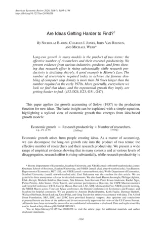
  • 13. 1116 THE AMERICAN ECONOMIC REVIEW APRIL 2020 of research effort already incorporates a ­market-based adjustment for the depletion of talent: R&D spending weights workers according to their wage, and less talented researchers will naturally earn a lower salary. If more of these ­workers are hired over time, R&D spending will not rise by as much. Second, adjusting for ​λ​only affects the magnitude of the trend in research productivity, not the overall qualitative fact of whether or not there is a downward trend. It is easy to deflate the growth rate of research effort by any particular value of ​λ​to get a sense for how this matters; cut- ting our growth rates in half, an extreme adjustment, would still leave the nature of our results unchanged. Finally, there is no consensus on what value of ​λ​one should use: Kremer (1993) even considers the possibility that it might be larger than one because of network effects and Zeira (2011) shows how patent races and duplica- tion can occur even with ​λ =  1​. Nevertheless, the Appendix shows the robustness of the main results in the paper to our baseline assumption by considering the case of ​λ  = 3 / 4​. The remainder of the paper applies this framework in a wide range of different contexts: Moore’s Law for semiconductors, agricultural crop yields, pharmaceutical innovation and mortality, and then finally at the firm level using Compustat data. III.  Moore’s Law One of the key drivers of economic growth during the last half century is Moore’s Law: the empirical regularity that the number of transistors packed onto an inte- grated circuit serving as the central processing unit for a computer doubles approx- imately every two years. Figure 3 shows this regularity back to 1971. The log scale of this figure indicates the overall stability of the relationship, dating back nearly 50 years, as well as the tremendous rate of growth that is implied. Related formulations of Moore’s Law involving computing performance per watt of electricity or the cost of information technology could also be considered, but the transistor count on an integrated circuit is the original and most famous version of the law, so we use that one here. A doubling time of two years is equivalent to a constant exponential growth rate of 35 percent per year. We therefore measure the output of the idea production for Moore’s Law as a stable 35 percent per year. Other alternatives are possible. For example, we could use decadal growth rates or other averages, and some of these approaches will be employed later in the paper. However, from the stand- point of understanding steady, rapid exponential growth for nearly half a century, the ­stability implied by the straight line in Figure 3 is a good place to start. And any slowing of Moore’s Law would only reinforce the finding we are about to document.12 If the output side of Moore’s Law is constant exponential growth, what is ­happening on the input side? Many commentators note that Moore’s Law is not a law of nature but instead results from intense research effort: doubling the tran- sistor density is often viewed as a goal or target for research programs. We measure research effort by deflating the nominal semiconductor R&D expenditures of all the 12  For example, there is a recent shift away from speed and toward ­energy-saving features; see Flamm (2017) and Pillai (2016). However, our analysis still applies historically.
  • 14. 1117BLOOM ET AL.: ARE IDEAS GETTING HARDER TO FIND?VOL. 110 NO. 4 main firms by the nominal wage of ­high-skilled workers, as discussed above. Our semiconductor R&D series includes research spending by Intel, Fairchild, National Semiconductor, Motorola, Texas Instruments, Samsung, and more than two dozen other semiconductor firms and equipment manufacturers. More details are provided in the notes to Table 1 and in the online Appendix. The striking fact, shown in Figure 4, is that research effort has risen by a factor of 18 since 1971. This increase occurs while the growth rate of chip density is more or less stable: the constant exponential growth implied by Moore’s Law has been achieved only by a massive increase in the amount of resources devoted to pushing the frontier forward. Assuming a constant growth rate for Moore’s Law, the implication is that research productivity has fallen by this same factor of 18, an average rate of 6.8 percent per year. If the null hypothesis of constant research productivity were correct, the growth rate underlying Moore’s Law should have increased by a factor of 18 as well. Instead, it was remarkably stable. Put differently, because of declining research ­productivity, it is around 18 times harder today to generate the exponential growth behind Moore’s Law than it was in 1971. The top panel of Table 1 reports the robustness of this result to various assump- tions about which R&D expenditures should be counted. No matter how we measure R&D spending, we see a large increase in effective research and a corresponding large decline in research productivity. Even by the most conservative measure in the table, research productivity falls by a factor of 8 between 1971 and 2014. The bottom panel of Table  1 considers an alternative to Moore’s Law as the “idea output” measure, focusing instead on TFP growth in the “­semiconductor and related device manufacturing” industry (NAICS 334413) from the Figure 3. The Steady Exponential Growth of Moore’s Law Source: Wikipedia (2017) 2,600,000,000 1,000,000,000 100,000,000 10,000,000 1,000,000 100,000 10,000 2,300 1971 1980 1990 Transistorcount Date of introduction 2000 2011 Line shows transistor count doubling every two years
  • 15. 1118 THE AMERICAN ECONOMIC REVIEW APRIL 2020 NBER/CES Manufacturing Industry Database. Because of an acceleration in ­average TFP growth from around 8 percent per year to around 20 percent per year in the late 1990s, approximately a ­three-fold increase in the growth rate, these ­calculations show a slightly smaller decline in research productivity. Still, though, the increases in research effort are much larger than the increase in TFP growth, so research productivity falls substantially even using this alternative. Caveats Now is a good time to consider what could go wrong in our research produc- tivity calculation at the micro level. Mismeasurement on both the output and input sides are clearly a cause for concern in general. However, there are two specific measurement problems that are worth considering in more detail. First, suppose there are “spillovers” from other sectors into the production of new ideas related to semiconductors. For example, progress in a completely different branch of materials Table 1—Research Productivity for Moore’s Law Factor decrease Average growth (%) Implied half-life (years) Moore’s Law, 1971–2014 Baseline 18 −6.8 10.3 1. Narrow 8 −4.8 14.5 2. Narrow (downweight conglomerates) 11 −5.6 12.3 3. Broad (downweight conglomerates) 26 −7.6 9.1 4.  Intel only (narrow) 347 −13.6 5.1 5. Intel + AMD (narrow) 352 −13.6 5.1 TFP Growth in Semiconductors, 1975–2011 6. Narrow (no equipment R&D) 5 −3.2 21.4 7. Narrow (with equipment R&D) 7 −4.4 15.8 8. Broad (no equipment R&D) 11 −5.6 12.3 9. Broad (with equipment R&D) 13 −6.1 11.3 Notes: Research productivity is the ratio of idea output, either a constant 35 percent per year for the first panel or TFP growth in semiconductors for the second, to the effective number of researchers. The effective number of researchers is measured by deflating the nominal semiconductor R&D expenditures of key firms by the aver- age wage of high-skilled workers. The R&D measures are based on Compustat (2016) data and PATSTAT data, assembled with assistance from Unni Pillai and Antoine Dechezlepretre. We start with the R&D spending data on 30 semiconductor firms plus an additional 11 semiconductor equipment manufacturers from all over the world. Next, we gathered data from PATSTAT on patents from the US patent office. The different rows in this table differ in how we add up the data across firms. There are two basic ways we treat the R&D data. In the Narrow treatment, we recognize that firms engage in different kinds of R&D, only some of which may be relevant for Moore’s Law. We therefore weight a firm’s R&D according to a (moving average) of the share of its patents that are in semicon- ductors (IPC group “H01L”). For example, in 1970, 75 percent of Intel’s patents were for semiconductors, but by 2010 this number had fallen to just 8 percent. In the Broad category, we include all R&D by semiconductor firms like Intel and National Semiconductor but use the patent data to infer semiconductor R&D for conglomerates like IBM, RCA, Texas Instruments, Toshiba, and Samsung. The downweight conglomerates label means that we further downweight the R&D spending of conglomerates and newer firms like Micron and SK Hynix that focus on mem- ory chips or chips for HDTVs and automobiles by a factor of 1/2, reflecting the possibility that even their semicon- ductor patenting data may be broader than Moore’s Law. Rows 4 and 5 show results when we consider the Narrow measure of R&D but focus on only one or two firms. Rows 6 through 9 undertake the calculation using TFP growth in the “semiconductor and related device manufacturing” industry (334413) from the NBER/CES Manufacturing Industry Database; see Bartelsman and Gray (1996). We smooth TFP growth using the HP filter and lag R&D by 5 years in this calculation. In addition to the narrow/broad split, we also include and exclude R&D from semicon- ductor equipment manufacturers in this calculation (equipment is captured in a separate 6-digit industry, but there may be spillovers). See the online Appendix for more details. The implied half life is the number of years that it takes research productivity to fall in half at the measured growth rate.
  • 16. 1119BLOOM ET AL.: ARE IDEAS GETTING HARDER TO FIND?VOL. 110 NO. 4 science may lead to a new idea that improves computer chips. Such positive spill- overs are not a problem for our analysis; instead, they are one possible factor that our research productivity measure captures. Of course, other things equal, positive spillovers would show up as an increase in research productivity rather than as the declines that we document in this paper. Alternatively, if such spillovers were larger at the start of our time period than at the end, then this would be one possible story for why research productivity has declined.13 A type of measurement error that could cause our findings to be misleading is if we systematically understate R&D in early years and this bias gets corrected over time. In the case of Moore’s Law, we are careful to include research spending by firms that are no longer household names, like Fairchild Camera and Instrument (later Fairchild Semiconductor) and National Semiconductor so as to minimize this bias: for example, in 1971, Intel’s R&D was just 0.4 percent of our estimate for total semiconductor R&D in that year. Throughout the paper, we try to be as careful as we can with measurement issues, but this type of problem must be acknowledged. IV.  Agricultural Crop Yields Our next application for measuring research productivity is agriculture. Due partly to the sector’s historical importance, crop yields and agricultural R&D spending are relatively ­well measured. We begin in Figure 5 by showing research ­productivity for the agriculture sector as a whole. As our “idea output” measure, we use (a smoothed 13  Lucking, Bloom, and Van Reenen (2017) provides an analysis of R&D spillovers using US ­firm-level data over the last three decades. They find evidence that knowledge spillovers are substantial, but have been broadly stable over time. Figure 4. Data on Moore’s Law Notes: The effective number of researchers is measured by deflating the nominal semiconductor R&D expenditures of key firms by the average wage of ­high-skilled workers and is normalized to 1 in 1970. The R&D data include research by Intel, Fairchild, National Semiconductor, Texas Instruments, Motorola, and more than two dozen other semiconductor firms and equipment manufacturers; see Table 1 for more details. 0% 35% Effective number of researchers (right scale)Growthrate 1 5 10 1970 1975 1980 1985 1990 1995 2000 2005 2010 2015 15 20 Factorincreasesince1971 A˙it/Ait (left scale)
  • 17. 1120 THE AMERICAN ECONOMIC REVIEW APRIL 2020 version of ) total factor productivity growth over the next five years. TFP growth declines slightly in agriculture, while effective research rises by about a factor of two between 1970 and 2007. Research productivity therefore declines over this period by a factor of nearly four, or at an average annual rate of 3.7 percent per year. We now turn to the main focus of this section, research productivity for various agricultural crops. Ideally, we would use total factor productivity by crop as our idea output measure. Unfortunately, such a measure is not available because farms are “multiple input, multiple output” enterprises in which capital, labor, materials, and energy inputs are not easily allocated to individual crops. Instead, we use the growth rate of yield per acre as our measure of idea output. For the agriculture sector as a whole, growth in yield per acre and total factor productivity look similar. For each of corn, soybeans, cotton, and wheat, we obtain data on both crop yields and R&D expenditures directed at improving crop yields. Figure 6 shows the annualized average ­5-year growth rate of yields (after smoothing to remove shocks mostly due to weather).Yield growth has averaged around 1.5 percent per year since 1960 for these four crops, but with ample heterogeneity. These ­5-year growth rates serve as our measure of idea output in studying the idea production function for seed yields. The green lines in Figure 6 show measures of the “effective” number of research- ers focused on each crop, measured as the sum of public and private R&D spend- ing deflated by the wage of ­high-skilled workers. Two measures are presented. The ­faster-rising number corresponds to research targeted only at ­so-called bio- logical efficiency. This includes ­cross-breeding (hybridization) and genetic mod- ification directed at increasing yields, both directly and indirectly via improving insect resistance, herbicide tolerance, and efficiency of nutrient uptake, for exam- ple. The ­slower-growing number additionally includes research on crop protection Figure 5. TFP Growth and Research Effort in Agriculture Notes: The effective number of researchers is measured by deflating nominal R&D expenditures by the average wage of ­high-skilled workers. Both TFP growth and US R&D spending (public and private) for the agriculture ­sector as a whole are taken from the US Department of Agriculture Economic Research Service (2018a, b). The TFP series is smoothed with an HP filter. Global R&D spending for agriculture is taken from Fuglie et al. (2011), Beintema et al. (2012), and Pardey et al. (2016). 0 2 4 TFP growth, left scale (next 5 years) US researchers (1970 = 1, right scale) Global researchers (1980 = 1, right scale) Growthrate 1 1.5 2 Factorincrease 1950 1960 1970 1980 1990 2000 2010
  • 18. 1121BLOOM ET AL.: ARE IDEAS GETTING HARDER TO FIND?VOL. 110 NO. 4 and ­maintenance, which includes the development of herbicides and pesticides. The effective number of researchers has grown sharply since 1969, rising by a factor that ranges from 3 to more than 25, depending on the crop and the research measure.14 It is immediately evident from Figure  6 that research productivity has fallen sharply for agricultural yields: yield growth is relatively stable or even declining, while the effective research that has driven this yield growth has risen tremendously. Research productivity is simply the ratio of average yield growth divided by the number of researchers. Table 2 summarizes the research productivity calculation for seed yields. As already noted, the effective number of researchers working to improve seed yields rose enormously between 1969 and 2009. For example, the increase was more than a factor of 23 for both corn and soybeans when research is limited to seed effi- ciency. If yield growth were constant (which is not a bad approximation across the four crops as shown in Figure 6), then research productivity would on average 14  Our measure of R&D inputs consists of the sum of R&D spending by the public and private sectors in the United States. Data on private sector biological efficiency and crop protection R&D expenditures are from an updated USDA series based on Fuglie et al. (2011), with the distribution of expenditure by crop taken from Perrin, Kunnings, and Ihnen (1983); ­Fernandez-Cornejo et al. (2004); Traxler et al. (2005); Huffman and Evenson (2006); and Centre for Industry Education Collaboration (2016). Data on US public sector R&D expenditure by crop are from the US Department of Agriculture National Institute of Food and Agriculture Current Research Information System (2016) and Huffman and Evenson (2006), with the distribution of expenditure by research focus taken from Huffman and Evenson (2006). Figure 6.Yield Growth and Research Effort by Crop Notes: The blue line is the annual growth rate of the smoothed crop yields over the following 5 years; national real- ized yields for each crop are taken from the US Department of Agriculture National Agricultural Statistics Service (2016). The two green lines report effective research: the solid line is based on R&D targeting seed efficiency only; the dashed lower line additionally includes research on crop protection. Both are ­normalized to 1 in 1969. R&D expenditures are deflated by a measure of the nominal wage for ­high-skilled ­workers. See the online Appendix for more details. 0% 4% 8% 12% 16% Yield growth, left scale (moving average) Yield growth, left scale (moving average) Effective number of researchers (right scale) Yield growth, left scale (moving average) Effective number of researchers (right scale) Yield growth, left scale (moving average) Effective number of researchers (right scale) Effective number of researchers (right scale) GrowthrateGrowthrate 0% 4% 8% 12% 16% GrowthrateGrowthrate 0 6 12 18 24 0 2 4 6 8 0 4 8 12 0 6 12 18 24 Factorincreasesince1969 Factorincreasesince1969Factorincreasesince1969 Factorincreasesince1969 Panel A. Corn Panel B. Soybeans Panel C. Cotton Panel D. Wheat 0% 2% 4% 6% 8% 0% 2% 4% 6% 8% 1960 1970 1980 2000 20101990 1960 1970 1980 2000 20101990 1960 1970 1980 2000 201019901960 1970 1980 2000 20101990
  • 19. 1122 THE AMERICAN ECONOMIC REVIEW APRIL 2020 decline by this same factor. The last 2 columns of Table 2 show this to be the case. On average, research productivity declines for crop yields by about 6 percent per year using the narrow definition of research and by about 4 percent per year using the broader definition. A potential source of mismeasurement for this case relates to the quality of land inputs. What if researchers are devoting their efforts to bringing ­lower-quality land into production? This could show up as a decrease in average yields, even as research is increasing yields for any given quality of land. First, at a high level, it’s worth noting that the total acreage of cotton and wheat planted in the United States has declined over our time period. (By contrast, acreage devoted to soybeans has doubled, while that for corn has increased slightly.) The declining acreage for cotton and wheat, and roughly constant acreage for corn, does not suggest on the face of it that changes on the extensive margin for those crops are crucial. Moreover, in order for what we find to be consistent with constant research productivity, we’d need average yields in the absence of research to be falling (due to lower land quality, say) at a rate that is growing exponentially in magnitude. This also seems unlikely. As an additional robustness check, we calculated our measures of research produc- tivity using ­state-level estimates of seed yield growth as our idea output measure (maintaining our broad research effort measure, since the nonrivalry of ideas means that research everywhere could be relevant for seed yields in each state). We found that, for each crop, the vast majority of individual states experienced declines in research productivity over our time period, mirroring the ­national-level results. V.  Mortality and Life Expectancy Health expenditures account for around 18 percent of US GDP, and a healthy life is one of the most important goods we purchase. Our third collection of case studies examines the productivity of medical research. Table 2—Research Productivity in Agriculture, 1969–2009 Effective research Research productivity Factor increase Avg. growth (%) Factor decrease Avg. growth (%) Research on seed efficiency only  Corn 23.0 7.8 52.2 −9.9  Soybeans 23.4 7.9 18.7 −7.3  Cotton 10.6 5.9 3.8 −3.4  Wheat 6.1 4.5 11.7 −6.1 Research includes crop protection  Corn 5.3 4.2 12.0 −6.2  Soybeans 7.3 5.0 5.8 −4.4  Cotton 1.7 1.3 0.6 +1.3  Wheat 2.0 1.7 3.8 −3.3 Agriculture   US research, 1970–2008 1.9 1.8 3.9 −3.7   Global research, 1980–2010 1.6 1.6 5.2 −5.5 Notes: Research productivity is the ratio of idea output, yield growth, to the effective number of researchers, mea- sured as R&D expenditures deflated by the nominal wage for high-skilled workers. In the first panel of results, the research input is based on R&D expenditures for seed efficiency only. The second panel additionally includes research on crop protection. See the online Appendix for more details.
  • 20. 1123BLOOM ET AL.: ARE IDEAS GETTING HARDER TO FIND?VOL. 110 NO. 4 A. New Molecular Entities Our first example from the medical sector is a fact that is ­well known in the litera- ture, recast in terms of our research productivity calculation. New molecular entities (NMEs) are novel compounds that form the basis of new drugs. Historically, the number of NMEs approved by the Food and Drug Administration each year shows little or no trend, while the number of dollars spent on pharmaceutical research has grown dramatically; for example, see Akcigit and Liu (2016). We reexamine this fact using our measure of research productivity, i.e., deflating pharmaceutical research by the ­high-skilled wage. The details of this calculation are reported in the online Appendix. The result is that research effort rises by a factor of 9, while research productivity falls by a factor of 11 by 2007 before rising in recent years so that the overall decline by 2014 is a factor of 5. Over the entire period, research effort rises at an annual rate of 6.0 percent, while research productivity falls at an annual rate of 3.5 percent. Of course, it is far from obvious that simple counts of NMEs appropriately measure the output of ideas; we would really like to know how important each innovation is. In addition, NMEs suffer from an important aggre- gation issue, adding up across a wide range of health conditions. These limitations motivate the approach described next, where we turn to the productivity of medical research for specific diseases. B. Years of Life Saved To measure idea output in treating diseases, we begin with life expectancy. Figure 7 shows US life expectancy at birth and at age 65. This graph makes the important point that life expectancy is one of the few economic goods that does not exhibit exponential growth. Instead, arithmetic growth is a better description. Since 1950, US life expectancy at birth has increased at a relatively stable rate of 1.8 years each decade, and life expectancy at age 65 has risen at 0.9 years per decade. Linear increases in life expectancy seem to coincide with stable economic growth.15 Also shown in the graph is the ­well-known fact that overall life expectancy grew even more rapidly during the first half of the twentieth century, at around 3.8 years per decade. This raises the question of whether even arithmetic growth is an appro- priate characterization. We believe that it is for two reasons. First, there is no sign of a slowdown in the years gained per decade since 1950, either in life expectancy at birth or in life expectancy at age 65. The second reason is a fascinating empir- ical regularity documented by Oeppen and Vaupel (2002). That paper shows that “record female life expectancy,” the life expectancy of women in the country for which they live the longest, has risen at a remarkably steady rate of 2.4 years per decade ever since 1840. Steady linear increases in life expectancy, not exponential ones, seem to be the norm. For this reason, we use “years of life saved,” that is, the change in life expectancy rather than its growth rate, as a measure of idea output. Because the growth rate of life expectancy is declining, our results would be even stronger under that alternative. 15  For example, see Nordhaus (2003), Hall and Jones (2007), and ­Dalgaard and Strulik (2014).
  • 21. 1124 THE AMERICAN ECONOMIC REVIEW APRIL 2020 C. Years of Life Saved from Specific Diseases To measure the years of life saved from reductions in ­disease-specific ­mortality, consider a person who faces two ­age-invariant Poisson processes for dying, with arrival rates ​​δ​1​​​and ​​δ​2​​​. We think of ​​δ​1​​​as reflecting a particular disease we are ­studying, such as cancer or heart disease, and ​​δ​2​​​as capturing all other sources of mor- tality. The probability a person lives for at least ​x​years before succumbing to type ​i​ mortality is the survival rate ​​S​  i​​​(x)​  =  ​e​​ −​δ​i​​ x ​​, and the probability the person lives for at least ​x​years before dying from any cause is ​S​(x)​  =  ​S​ 1​​​(x)​ ​S​  2​​​(x)​  =  ​e​​ −​(​δ​1​​+​δ​2​​)​x ​​. Life expectancy at age ​a​, ​LE​(a)​​is then well known to equal (15) ​LE​(a)​  = ​∫ 0 ​  ∞ ​​S​(x)​ d x  = ​∫ 0 ​  ∞ ​​​e​​ −​(​δ​1​​+​δ​2​​)​ x ​ d x  =  ​  1 _  ​δ​1​​ + ​δ​2​​  ​​ . Now consider how life expectancy changes if the type ​i​mortality rate changes slightly. It is easy to show that the expected years of life saved by the mortality change is (16) ​dLE​(a)​  =  ​  ​δ​i​​  _  ​δ​1​​ + ​δ​2​​  ​ ⋅ LE​(a)​ ⋅ ​ ( − ​  d​δ​i​​  _  ​δ​i​​  ​ ) ​​ . That is, the expected years of life saved from a decline in, say, cancer mortality is the product of three terms. First is the fraction of deaths that result from cancer. Second is the average years of life lost if someone dies from cancer at age ​a​, and the final term is the percentage decline in cancer mortality.16 16  Our measures of life expectancy and mortality from all sources by age come from the Human Mortality Database (2016) (http://mortality.org). To measure the percentage declines in mortality rates from cancer, we use the ­age-adjusted mortality rates for people ages 50 and over computed from ­5-year survival rates, taken from the National Cancer Institute’s Surveillance, Epidemiology, and End Results program (http://seer.cancer.gov/). Figure 7. United States Life Expectancy Sources: National Center for Health Statistics (2014) and Clio Infra (2016) 1900 1920 1940 1960 1980 2000 45 50 55 60 65 70 75 80 At birth (left scale) At age 65 (right scale) Years Years 13 14 15 16 17 18 19 20
  • 22. 1125BLOOM ET AL.: ARE IDEAS GETTING HARDER TO FIND?VOL. 110 NO. 4 Vaupel and ­Canudas Romo (2003) shows that this expression generalizes to a much richer setting. In particular, the expected years of life saved is the product of three terms with the same interpretation. For example, they allow for an arbitrary number of causes of death each of which has a mortality rate that varies arbitrarily with age.17 The research input aimed at reducing mortality from a given disease is at first blush harder to measure. For example, it is difficult to get research spending bro- ken down into spending on various diseases. Nevertheless, we implement a poten- tial solution to this problem by measuring the number of scientific publications in PubMed that have “Neoplasms,” for example, as a MeSH (Medical Subject Heading) term. MeSH is the National Library of Medicine’s controlled vocabulary thesau- rus.18 We do this in two ways. Our broader approach (publications) uses all pub- lications with the appropriate MeSH keyword as our input measure. Our narrower approach (trials) further restricts our measure to those publications that according to MeSH correspond to a clinical trial. Rather than using scientific publications as an output measure, as other studies have done, we use publications and clinical trials as input measures to capture research effort aimed at reducing mortality for a particular disease.19 Figure 8 shows our basic “idea output” and “idea input” measures for mortality from all cancers, from breast cancer, and from heart disease. Heart disease and can- cer are the top two leading causes of death in the United States, and in the spirit of looking as narrowly as possible, we also chose to look at breast cancer mortality. For the two cancer types, we use the ­5-year mortality rate conditional on being diag- nosed with either type of cancer and see an ­S-shaped decline since 1975. This trans- lates into a ­hump-shaped Years of life saved per 1,000 people, the empirical analog of equation (16). For example, for all cancers, the years of life saved series peaks around 1990 at more than 100 years of life saved per 1,000 people before declining to around 60 years in the 2000s. For heart disease, a substantial part of the decline in deaths comes from people not contracting the disease in the first place, so we focus on the (smoothed) crude death rate for people aged 55 to 64. The death rate declines at different rates in different periods, leading to a series of humps in years of life saved, but overall there is no large trend in this measure of idea output. The right panels of Figure 8 show our research input measure based on PubMed publication statistics. Total publications for all cancers increased by a factor of 3.5 between 1975 and 2006 (the years for which we’ll be able to compute research productivity), while publications restricted to clinical trials increased by a factor of 17  Their formula involves an extra covariance term as well. In particular, the covariance between the ­age-specific percentage decline in mortality associated with cancer and the years of life saved at age ​a​when cancer is averted. When the percentage decline in mortality rates is the same across ages, this covariance is zero. More generally, it can differ from zero, but in many of the calculations in their paper, the covariance is small. 18  For more information on MeSH, see https://www.nlm.nih.gov/mesh/. Our queries of the PubMed data use the webtool created by the Institute for Biostatistics and Medical Informatics (IBMI) Medical Faculty, University of Ljubljana, Slovenia (available at http://webtools.mf.­uni-lj.si/). 19  In independent work, Lichtenberg (2017) takes a similar approach in an econometric framework for the years 1999–2013. He uses a ­difference-in-differences specification to document an ­economically-significant correlation between research publications related to various cancer sites and subsequent mortality and years of life saved. Lichtenberg (2018) extends this approach further back in time to the period 1946–2015 and continues to find a relationship between publications and ­5-year survival rates.
  • 23. 1126 THE AMERICAN ECONOMIC REVIEW APRIL 2020 14.1 during this same period. A similar pattern is seen for research on breast cancer and heart disease. Research productivity for our medical research applications is computed as the ratio of years of life saved to the number of publications. Figure 9 shows our research productivity measures. The hump shape present in the ­years-of-life-saved measure carries over here. Research productivity rises until the mid-1980s and then falls. Overall, between 1975 and 2006, research productivity for all cancers declines by a factor of 1.2 using all publications and a factor of 4.8 using clinical trials. The declines for breast cancer and heart disease are even larger, as shown in Table 3. Figure 8. Mortality,Years of Life Saved, and Research Effort Notes: For the two cancer panels, the mortality rate is computed as negative the log of the (smoothed) ­five-year sur- vival rate for cancer for people ages 50 and higher, from the National Cancer Institute’s Surveillance, Epidemiology, and End Results program at http://seer.cancer.gov/. For heart disease, we report the crude death rate in each year for people aged 55–64. Years of life saved per 1,000 people is computed using equation (16), as described in the text. Research effort is measured by the number of related publications and clinical trials, taken from the PubMed publi- cations database. For publications, the research input is based on all publications in PubMed with “Neoplasms” or “Breast Neoplasms” or “Heart Diseases” as a MeSH keyword. The lines for “clinical trials” restrict further to pub- lications involving clinical trials. 0.3 0.4 1975 1980 1985 1995 2000 2005 2010 1990 1975 1980 1985 1995 2000 2005 2010 1990 1975 1970 1965 1980 1985 1995 2000 2005 2010 2015 1990 1960 1970 1980 2000 2010 2020 1990 1960 1970 1980 2000 2010 2020 1990 1960 1970 1980 2000 2010 2020 1990 0.5 0.6 0.7 0.8 Years of life saved per 1,000 people (right scale) Years of life saved per 1,000 people (right scale) Years of life saved per 1,000 people (right scale) Mortality rate (left scale) Mortality rate (left scale) Mortality rate (left scale) DeathrateDeathrateDeathrate 20 40 60 80 100 120 YearsYearsYears 25 100 400 1,600 6,400 25,600 102,400 Number of publications Number for clinical trials ResearcheffortResearcheffortResearcheffort Panel A. All cancers 0.05 0.1 0.15 0.2 0.25 0.3 0.35 5 10 15 20 25 30 35 25 50 100 200 400 800 1,600 3,200 6,400 12,800 Number of publications Number for clinical trials Panel B. Breast cancer 0.002 0.004 0.006 0.008 0.01 0.012 0.014 0.016 0.018 120 130 140 150 160 170 180 190 200 25 100 400 1,600 6,400 25,600 102,400 Number of publications Number for clinical trials Panel C. Heart disease
  • 24. 1127BLOOM ET AL.: ARE IDEAS GETTING HARDER TO FIND?VOL. 110 NO. 4 Several general comments about research productivity for medical research deserve mention. First, for this application, the units of research productiv- ity are ­diff­erent than what we’ve seen so far. For example, between 1985 and 2006, ­declining research productivity means that the number of years of life saved per 100,000 people in the population by each publication of a clinical trial related to cancer declined from more than 8 years to just over one year. For breast cancer, the changes are even starker: from around 16 years per clinical trial in the mid-1980s to less than 1 year by 2006. Figure 9. Research Productivity for Medical Research Note: Research productivity is computed as the ratio of years of life saved to the number of publications. Per clinical trial Per 100 publications 1 2 4 8 16 32 Yearsoflifesaved per100,000people Yearsoflifesaved per100,000people Yearsoflifesaved per100,000people Panel A. All cancers Per clinical trial Per 100 publications 1/2 1 2 4 8 16 32 64 128 256 Panel B. Breast cancer Per clinical trial Per 100 publications 4 8 16 32 64 128 256 Panel C. Heart disease 1975 1970 1980 1985 1995 2000 2005 2010 2015 1990 1975 1980 1985 1995 2000 2005 2010 1990 1975 1980 1985 1995 2000 2005 2010 1990 Table 3—Research Productivity for Medical Research Effective research Research productivity Disease Factor increase Avg. growth (%) Factor decrease Avg. growth (%) All publications   Cancer, all types 3.5 4.0 1.2 −0.6   Breast cancer 5.9 5.7 8.2 −6.8   Heart disease 5.1 3.6 5.3 −3.7 Clinical trials only   Cancer, all types 14.1 8.5 4.8 −5.1   Breast cancer 16.3 9.0 22.6 −10.1   Heart disease 24.2 7.1 25.3 −7.2 Notes: Research productivity is computed as the ratio of years of life saved to the number of publications. In the first panel, the research input is based on all publications in PubMed with “Neoplasms” or “Breast Neoplasms” or “Heart Diseases” as a MeSH keyword. The second panel restricts to only publications involving clinical trials. Results for cancer and breast cancer cover the years 1975–2006, while those for heart disease apply to 1968–2011. See the online Appendix for more details.
  • 25. 1128 THE AMERICAN ECONOMIC REVIEW APRIL 2020 Next, however, notice that the changes were not monotonic if we go back to 1975. Between 1975 and the ­mid-1980s, research productivity for these two cancer research categories increased quite substantially. The production function for new ideas is obviously complicated and heterogeneous. These cases suggest that it may get easier to find new ideas at first before getting harder, at least in some areas. VI.  Research Productivity in ­Firm-Level Data Our studies of semiconductors, crops, and health are illuminating, but at the end of the day, they are just case studies. One naturally wonders how representative they are of the broader economy. In addition, some growth models associate each firm with a different variety: perhaps the number of firms making corn or semiconduc- tor chips is rising sharply, so that research effort per firm is actually constant, as is research productivity at the firm level. Declining research productivity for corn or semiconductors could in this view simply reflect a further composition bias.20 To help address these concerns, we report two sets of results with ­firm-level data. Our first set is Compustat (2016) data on US ­publicly-traded firms. Our second set is ­administrative data from the Census of Manufacturing. Each dataset has its strengths. Compustat includes a longer time series as well as firms from outside manufacturing. The Census covers the universe of manufacturing firms rather than just those that are publicly traded. The strength of the ­firm-level data is that they are more representative than the case studies, but of course they too have limitations. ­Publicly-traded firms and man- ufacturing firms are each still a selected sample, and our measures of “ideas” and research inputs are likely to be less precise. And in some models, the product line rather than the firm is the right unit of observation. Creative destruction may make the ­firm-level results harder to interpret. This is because part of the effect of a firm’s own RD on its growth rate may reflect not just the impact on its productivity, but also a gain in market share at the expense of another firm (business stealing). Fortunately, empirical evaluations of the magnitude of R­D-induced business steal- ing using Compustat data find it to be quantitatively dominated by the knowledge creating effects of RD (see Bloom, Schankerman, and  Van Reenen 2013 and Lucking, Bloom, and Van Reenen 2017). With these caveats in mind, we view this ­firm-level evidence as a helpful complement to the case studies. A. Compustat Results As a measure of the output of the idea production function, we use decadal aver- ages of annual growth in sales revenue, market capitalization, employment, and revenue labor productivity within each firm. We take the decade as our period of observation to smooth out fluctuations. Why would growth in sales revenue, market cap, or employment be ­informative about a firm’s production of ideas? This approach follows a recent literature 20  For example, Peretto (1998, 2016b) emphasize this perspective on varieties, while Aghion and Howitt (1992) takes the alternative view that different firms may be involved in producing the same variety. Klette and Kortum (2004) allows the number of varieties produced by each firm to be heterogeneous and to evolve over time.
  • 26. 1129BLOOM ET AL.: ARE IDEAS GETTING HARDER TO FIND?VOL. 110 NO. 4 ­emphasizing precisely these links. Many papers have shown that news of patent grants for a firm has a large immediate effect on the firm’s stock market capital- ization (e.g., Blundell, Griffith, and Van Reenen 1999; Kogan et al. 2015). Patents are also positively correlated with the firm’s subsequent growth in employment and sales. More generally, in models in the tradition of Lucas (1978), Hopenhayn (1992), and Melitz (2003), increases in the fundamental productivity of a firm show up in the long run as increases in sales and firm size, but not as increases in sales reve- nue per worker.21 This motivates our use of sales revenue or employment to mea- sure fundamental productivity. Hsieh and Klenow (2009) and ­Garcia-Macia, Hsieh, and Klenow (2016) are recent examples of papers that follow a related approach. Of course, in more general models with fixed overhead labor costs for example, revenue labor productivity (i.e., sales revenue per worker) and TFPR can be related to fundamental productivity (e.g., Bartelsman, Haltiwanger, and Scarpetta 2013). And sales revenue and employment can change for reasons other than the discovery of new ideas. We try to address these issues by also looking at revenue productivity and through various sample selection procedures, discussed below. These problems also motivate the earlier approach of looking at case studies. To measure the research input, we use a firm’s spending on research and devel- opment from Compustat. This means we are restricted to ­publicly-listed firms that report formal RD, and such firms are ­well-known to be a select sample (e.g., disproportionately in manufacturing and large). We look at firms since 1980 that report ­nonzero RD, and this restricts us to an initial sample of 15,128 firms. Our ­additional requirements for sample selection in our baseline sample are: (i) We observe at least 3 annual growth observations for the firm in a given decade. These growth rates are averaged to form the idea output growth ­measure for that firm in that decade. (ii) We only consider decades in which our idea output growth measure for the firm is positive (negative growth is clearly not the result of the firm innovating). (iii) We require the firm to be observed (for both the output growth measure and the research input measure) for two consecutive decades. Our decades are the 1980s, the 1990s, the 2000s (which refers to the ­2000–2007 period), and the 2010s (which refers to the ­2010–2015 period); we drop the years 2008 and 2009 because of the financial crisis. We relax many of these conditions in our robustness checks. 21  This is obvious when one thinks about the equilibrium condition for the allocation of labor across firms in simple settings: in equilibrium, a worker must be indifferent between working in two different firms, which equal- izes wages. But wages are typically proportional to output per worker. Moreover, with ­Cobb-Douglas production and a common exponent on labor, sales revenue per worker would be precisely equated across firms even if they had different underlying productivities. In a Lucas (1978) span of control setting, more productive firms just hire more workers, which drives down the marginal product until it is equated across firms. In alternative settings with monopolistic competition, it is the price of a particular variety that declines as the firm expands. Regardless, higher fundamental productivity shows up as higher employment or sales revenue, but not in higher sales per employee.
  • 27. 1130 THE AMERICAN ECONOMIC REVIEW APRIL 2020 Table 4 shows our research productivity calculation for various cuts of the Compustat data. In all samples, there is substantial growth in the effective number of researchers within each firm, with growth rates averaging between 2.4 percent and 8.8 percent per year. Under our null hypothesis, this rapid growth in research should translate into higher growth rates of ­firm-level sales and employment with a constant level of research productivity. Instead, what we see in Table 4 are rapid declines in ­firm-level research productivity across all samples, at growth rates that range from −4.2 percent to −14.5 percent per year for multiple decades. Averaging across all our samples, research productivity falls at a rate of about 9  percent per year, cumulating to a 2.­5-fold decline every decade. At this rate, research productivity declines by a factor of about 15 over three decades of changes; put differently, it requires 15 times more researchers today than it did 30 years ago to produce the same rate of firm revenue growth. Figure 10 demonstrates the heterogeneity across firms in our Compustat sample by showing the distribution of the factor changes in effective research and research productivity across firms. In this figure, we focus on the results for sales revenue for firms observed for two decades, but the results with other output measures and other time horizons are similar; additional results are available in the online Appendix. The heterogeneity across firms is impressive and somewhat reminiscent of the heterogeneity we see in our case studies. Nevertheless, it is clear from the histogram that there is essentially no evidence that constant research productivity is Table 4—Research Productivity in Compustat Firm-Level Data Effective research Research productivity Sample Factor increase Avg. growth (%) Factor decrease Avg. growth (%) Sales revenue   2 decades (1,712 firms) 2.0 6.8 3.9 −13.6   3 decades (469 firms) 3.8 6.7 9.2 −11.1   4 decades (149 firms) 13.7 8.7 40.3 −12.3 Market cap   2 decades (1,124 firms) 2.2 8.0 3.4 −12.2   3 decades (335 firms) 3.1 5.6 6.3 − 9.2   4 decades (125 firms) 7.9 6.9 14.0 −8.8 Employment   2 decades (1,395 firms) 2.2 8.0 2.8 −10.3   3 decades (319 firms) 4.0 6.9 18.2 −14.5   4 decades (101 firms) 13.9 8.8 31.5 −11.5 Revenue labor productivity   2 decades (1,444 firms) 1.9 6.4 2.2 −7.9   3 decades (337 firms) 1.6 2.4 2.5 −4.5   4 decades (109 firms) 2.5 3.1 3.5 −4.2 Notes: The table shows averages of firm-level outcomes for effective research and research productivity. Sales rev- enue and Market cap are deflated by the GDP implicit price deflator. Revenue labor productivity is deflated Sales revenue divided by Employment. The effective number of researchers (Effective research) is measured by deflat- ing nominal RD expenditures by the average wage of high-skilled workers. The average growth rate across two decades is computed by dividing by ten years (e.g., between 1985 and 1995); others follow this same approach. Averages are computed by weighting firms by the median number of effective researchers in each firm across the decades. See the online Appendix for more details.
  • 28. 1131BLOOM ET AL.: ARE IDEAS GETTING HARDER TO FIND?VOL. 110 NO. 4 a good characterization of the ­firm-level data. The average, median, and modal firms experience large declines in research productivity. There is a long tail of firms expe- riencing even larger declines but also a small minority of firms that see increases in research productivity. The fraction of firms that exhibit something like constant research productivity is tiny. For example, less than 5 percent of firms across our three time frames have research productivity changing (either rising or falling) by less than 1 percent per year on average. Table 5 provides additional evidence of robustness. In the interests of brevity, we report these results for the sales revenue and for firms that we observe across three decades, but the results for our other output measures and time frames are similar. The first row repeats the benchmark results described earlier. The second and third rows relax the requirement that sales growth is positive. This increases the sample size considerably and brings the RD growth numbers down substantially. In both cases, research productivity falls sharply, reassuring us that this sample selection criteria is not driving the results. The fourth row imposes the restriction that research is increasing across the observed decades. The fifth row tightens our restrictions and drops firm in which sales revenue declines on average in any decade. The sixth row uses median sales growth rather than mean as our output measure. The seventh row reports unweighted averages rather than weighting firms by the effective ­number of researchers. And the eighth row uses ­so-called “DHS growth rates” defined ­following Davis, Haltiwanger, and Schuh (1996); this bounds growth rates between −2 and +2, addressing any concerns over outliers. The general finding of substan- tial declines in research productivity is robust. Figure 10. Compustat Distributions, Sales Revenue (Two Decades) Notes: Based on 1,712 firms. 22.1 percent of firms have increasing research productivity. Only 3.0 percent have research productivity that is roughly constant, defined as a growth rate whose absolute value is less than 1 percent per year. See Notes to Table 4 for more details. Number of researchers Research productivity 1/100,000 1/10,000 1/1,000 1/100 1/10 1 10 100 1,000 10,000 200 180 160 140 120 80 60 40 20 0 100 Numberoffirms Across two decades Factor change in research productivity and effective number of researchers
  • 29. 1132 THE AMERICAN ECONOMIC REVIEW APRIL 2020 B. Census of Manufacturing Results We also look at firms in the US Census of Manufacturing (Bureau of the Census 2015b), using data from the responses to mandatory survey responses on sales (Economic Census) and on RD activity (Bureau of the Census 2009, 2015a, SIRD/BRDIS). These data have a number of differences with Compustat which makes them a valuable robustness check. First, they use the responses to official (mandatory) government surveys, rather than audited financial accounts. So this could potentially induce some measurement error (if the auditing process helps to eliminate recording errors for example), but it also helps to address concerns over potential bias in reported accounting data for ­publicly-listed firms (e.g., if firms manipulate their reported RD activity to influence their stock market valuation). Second, they cover the activity of all firms operating in the United States, public and private, including the subsidiaries of foreign multinationals. Thus, smaller firms, ­start-ups, and subsidiaries of overseas firms are included.22 Third, the Census data exclude the RD and sales activities of US firms abroad, which for large manufactur- ing firms is often substantial. By contrast, Compustat reports the global ­consolidated accounts, so overseas sales and RD will be included in the totals.23 Fourth, the Census also collects data on the number of scientists and engineers engaged in RD activity, providing a quantity measure of innovation inputs. Finally, the Census com- pares the figures for large firms against administrative data, e.g., IRS tax returns and social security filings, helping to ensure data accuracy. Our sample includes all firms that reported manufacturing shipments (sales) in the Economic Censuses (CMF) of 1982, 1992, 2002, and 2012, as well as positive 22  Including the RD and performance of small firms is potentially important as many innovations may come from younger firms. For example, see Acs and Audretsch (1988). 23  The Compustat Segment data do provide some breakdowns by geography and sector, but these are not consis- tently reported over a long enough time period nor for enough firms (especially for RD) for our exercise. Table 5—Compustat Sales Data across Three Decades: Robustness Effective research Research productivity Case Factor increase Avg. growth (%) Factor decrease Avg. growth (%) Benchmark (469 firms) 3.8 6.7 9.2 −11.1 Winsorize g  0.01 (986 firms) 2.3 4.1 7.9 −10.3 Winsorize top/bottom (986 firms) 2.3 4.1 6.0 −8.9 Research must increase (356 firms) 5.1 8.1 11.6 −12.3 Drop if any negative growth (367 firms) 5.6 8.6 17.9 −14.4 Median sales growth (586 firms) 3.8 6.6 6.3 −9.2 Unweighted averages (469 firms) 3.8 6.7 9.2 −11.1 DHS growth rates (470 firms) 3.8 6.7 3.6 −6.4 Notes: Robustness results reported for the sample of changes across three decades. Winsorize g  0.01 means we replace any idea output measure that is less than 1  percent annually with a value of 1 percent. Winsorize top/bottom does this same thing but winsorizes an equal number of firms at the top of the idea output distri- bution. Research must increase means we require that the research measure be rising across the decades. Drop if any negative growth means we drop firms that have any decade (across our 1980–2015 period) in which average market cap growth is negative. Median sales growth uses the median of sales revenue growth in each decade rather than the mean. Unweighted averages gives each firm equal weight in computing sum- mary statistics, rather than weighting each firm by its effective number of researchers. DHS growth rates uses ​​(​y​ t​​ − ​y​ t−1​​)​ / ​(0.5 ×  ​y​ t​​ + 0.5 × ​y​ t−1​​)​​to compute the growth rate of research productivity at the firm level to reduce problems with small denominators.
  • 30. 1133BLOOM ET AL.: ARE IDEAS GETTING HARDER TO FIND?VOL. 110 NO. 4 RD expenditure in the BRDIS (or SIRD before 2008) surveys of RD in at least one year in each decade. The data span 1,300 firms over 2,700 observations (where numbers have been rounded for disclosure purposes). Research productivity results in the Census data are reported in Table 6 and are similar to what we saw in the Compustat sample. In row 1 we see that while effec- tive research inputs have risen by 1.6 percent a year on average research productivity has fallen by 7.8 percent between 1992 and 2012. Part of the explanation is that our early period includes the “new economy” while our later period includes the Great Recession; this is a limitation of the Census sample. In row 2 we winsorize the growth rate in sales from below at 1 percent, finding that research productivity now falls by 6 percent. In row 3 we winsorize both the top and the bottom of the distribution of sales growth by the same share and still find a substantial decline in research productivity of 4.9 percent. In row 4 rather than weight firms by mean RD spending over the 20 year window we provide unweighted results showing a larger decline of −8.1 percent. Finally, in row 5 we use the number of research scientists and engineers that is collected in the BRDIS/SIRD survey form as our measure of scientific input. This addresses any concerns over the deflator for RD inputs as we are using a quantity (number of scientists and engineers) input measure, and we find once again a significant decline in research productivity of 6 percent. VII. Discussion A. Summary and ­Semi-Endogenous Growth Theory The evidence presented in this paper concerns the extent to which a constant level of research effort can generate constant exponential growth, either in the economy as a whole or within relatively narrow categories, such as a firm or a seed type or a health condition. We provide consistent evidence that the historical answer to this question is “no”: as summarized in Table 7, research productivity is declining at a substantial rate in virtually every place we look. The table also provides a way to Table 6—Census of Manufacturing Results, across Two Decades (1992–2002, 2002–2012) Effective research Research productivity Case Factor increase Avg. growth (%) Factor decrease Avg. growth (%) 1. Benchmark 1.2 1.6 2.2 −7.8 2. Winsorize g  0.01 1.2 1.6 1.9 −6.0 3. Winsorize top/bottom 1.2 1.6 1.7 −4.9 4. Unweighted 1.0 0.0 1.9 −8.1 5. Research  = scientists 1.3 2.3 2.3 −6.0 Notes: Research productivity is the ten-year DHS growth in real sales divided by mean RD spending, deflated by the skilled wage, over those ten years. Research productivity growth is then calculated as the percent change in research productivity compared to ten years earlier. In row 2, idea output (sales growth) is winsorized from below at 1 percent. In row 3, idea output (sales growth) is winsorized from below at 1 percent and from above such that an equal number of firms are winsorized in each tail. In row 4, the mean is unweighted. In row 5, the denominator in research productivity is the number of scientists and engineers. In rows 1 to 3, the mean of the growth rate of RD is weighted by mean RD over the past 20 years. In row 5, the mean of the growth rate of scientists and engineers is weighted by mean RD over the past 20 years. Factor decrease is calculated as 1/(​1 − ​mean) where mean is the mean of the research productivity growth weighted by the average RD spending over the past 20 years. Average growth is calculated as ​1 − ​​(1 − mean)​​​ 1/10 ​​where mean is the mean of research productivity growth weighted by the average RD spending over the past 20 years. The sample includes 1,300 firms and 2,700 observations for all cells.