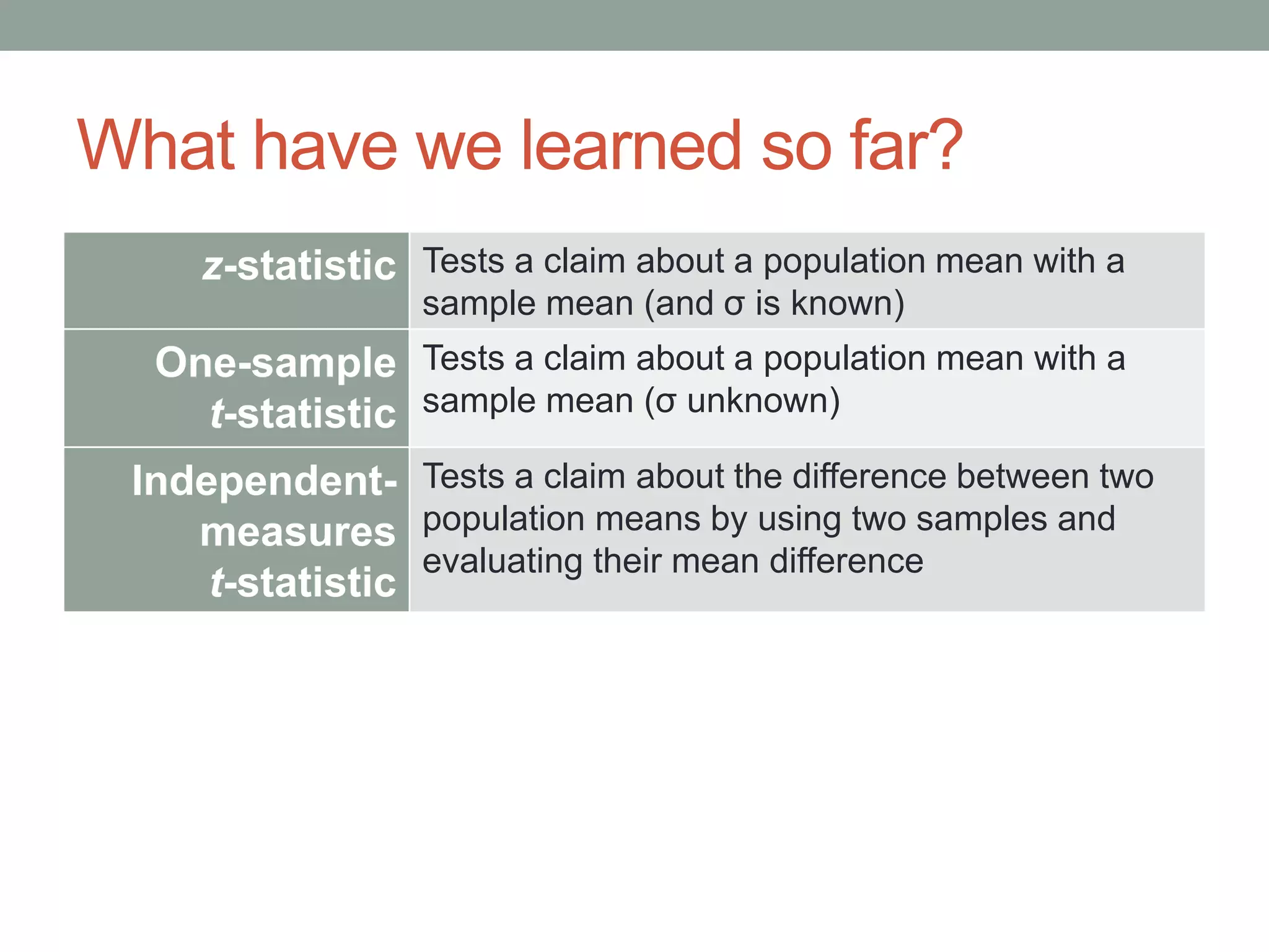
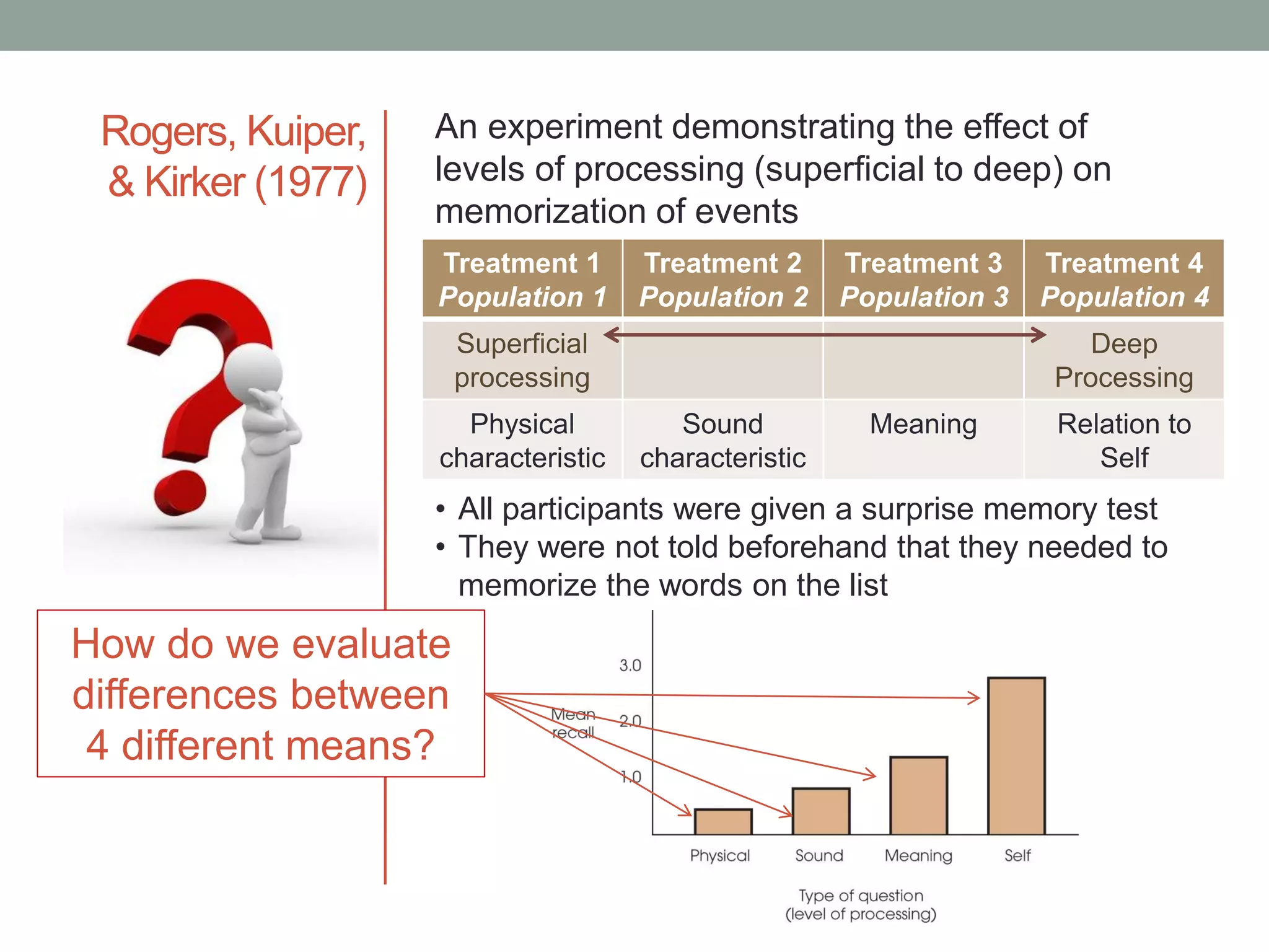
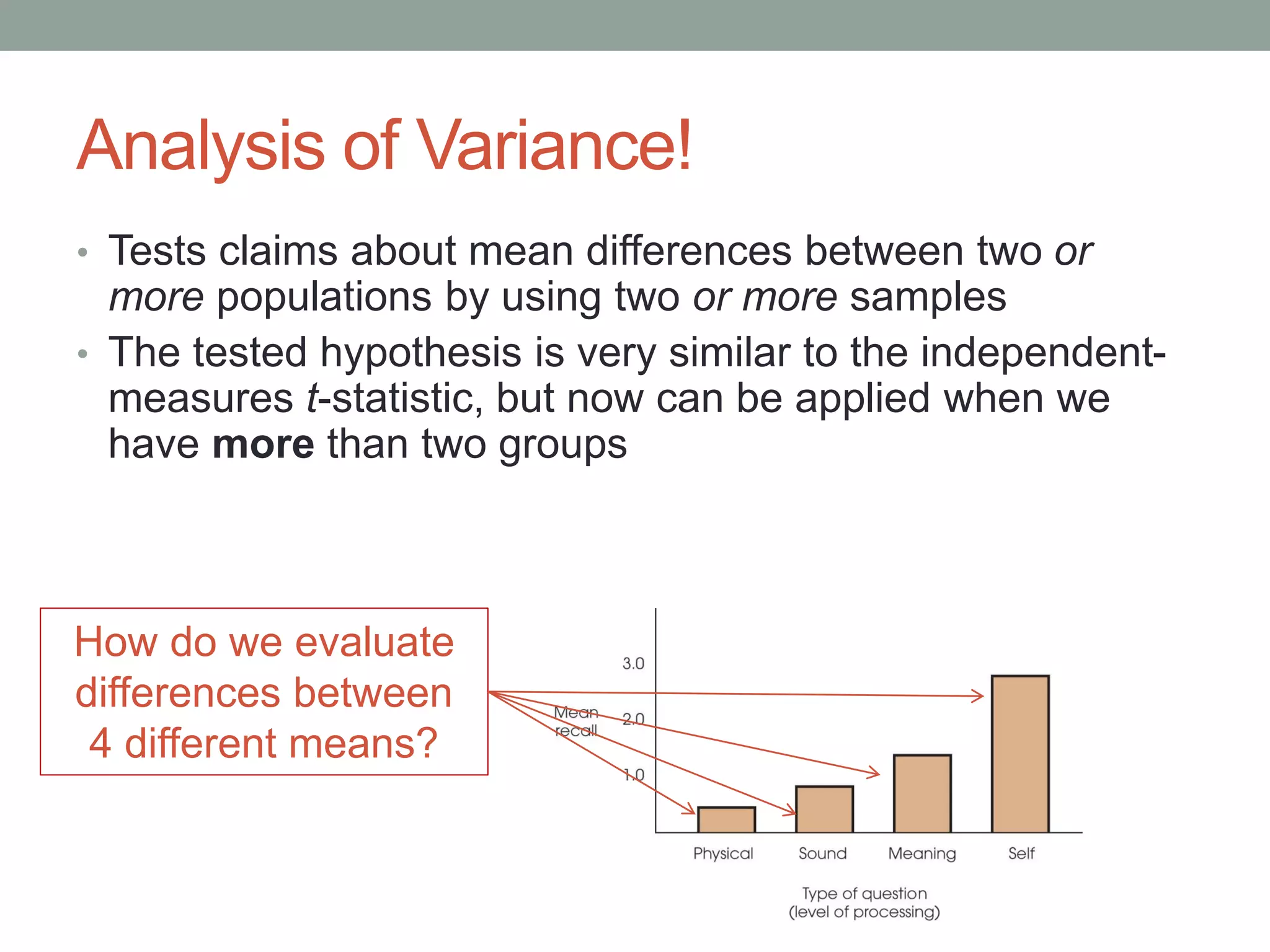
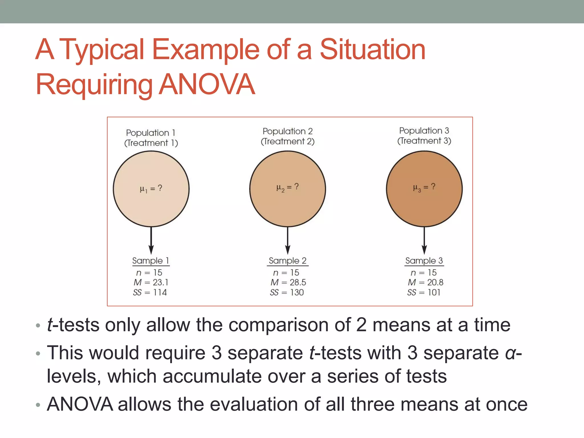
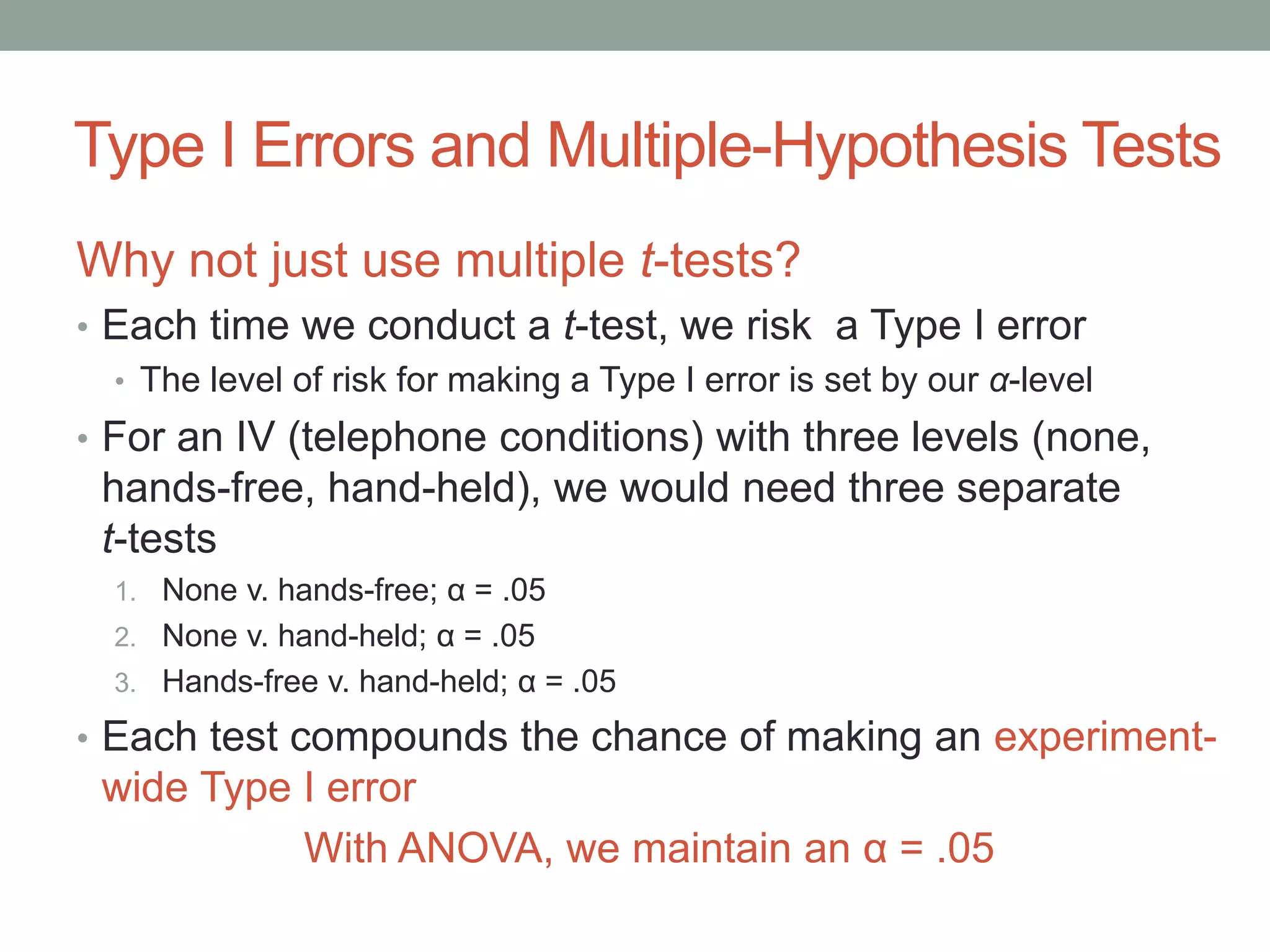
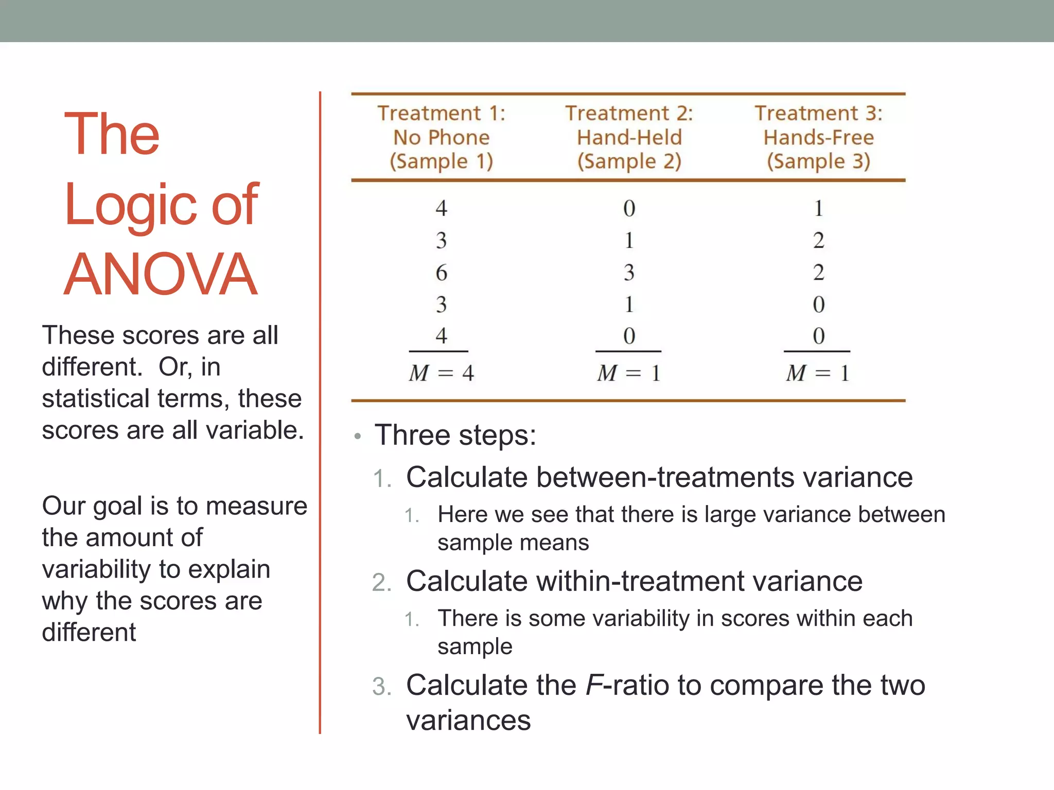
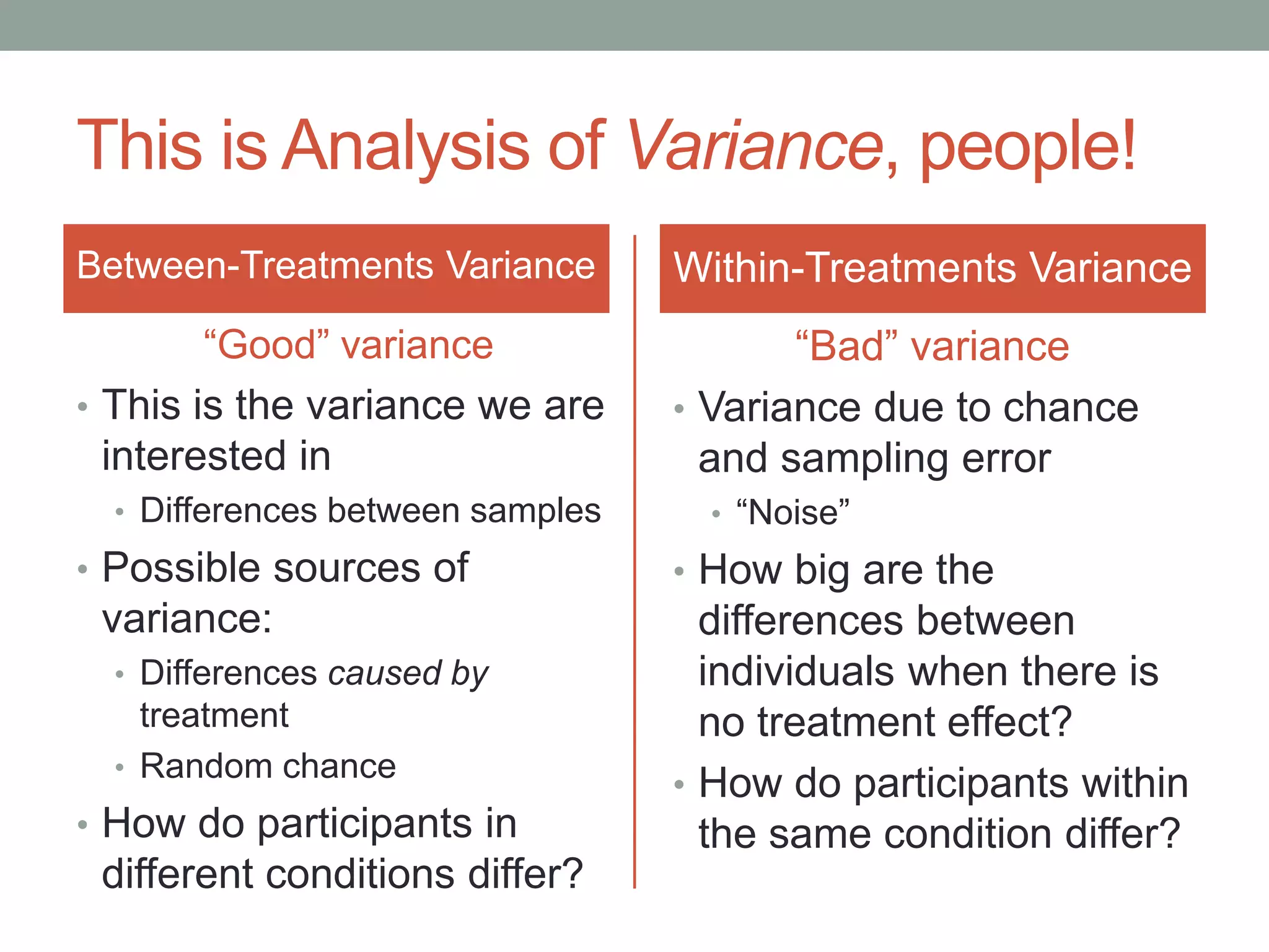
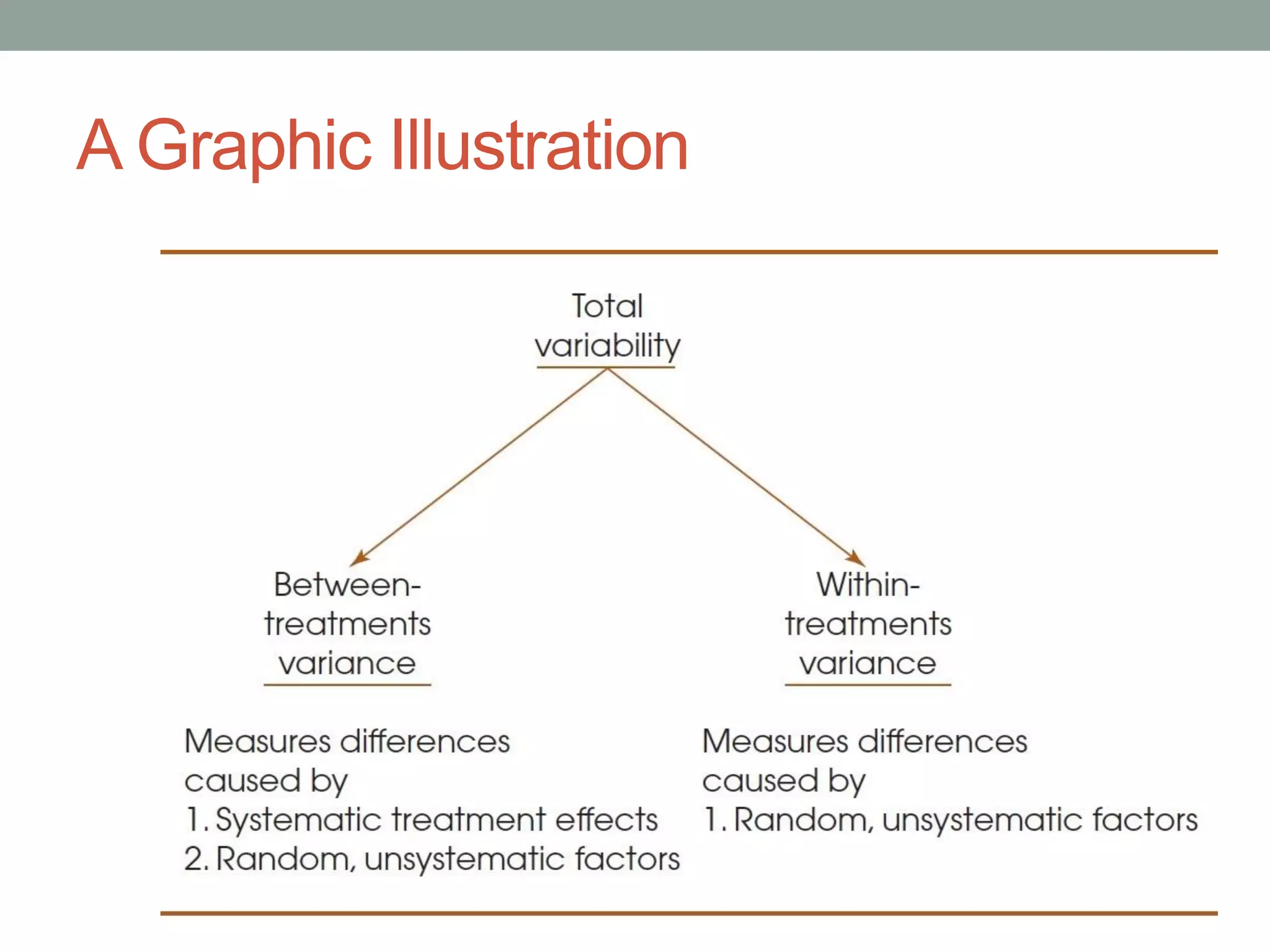
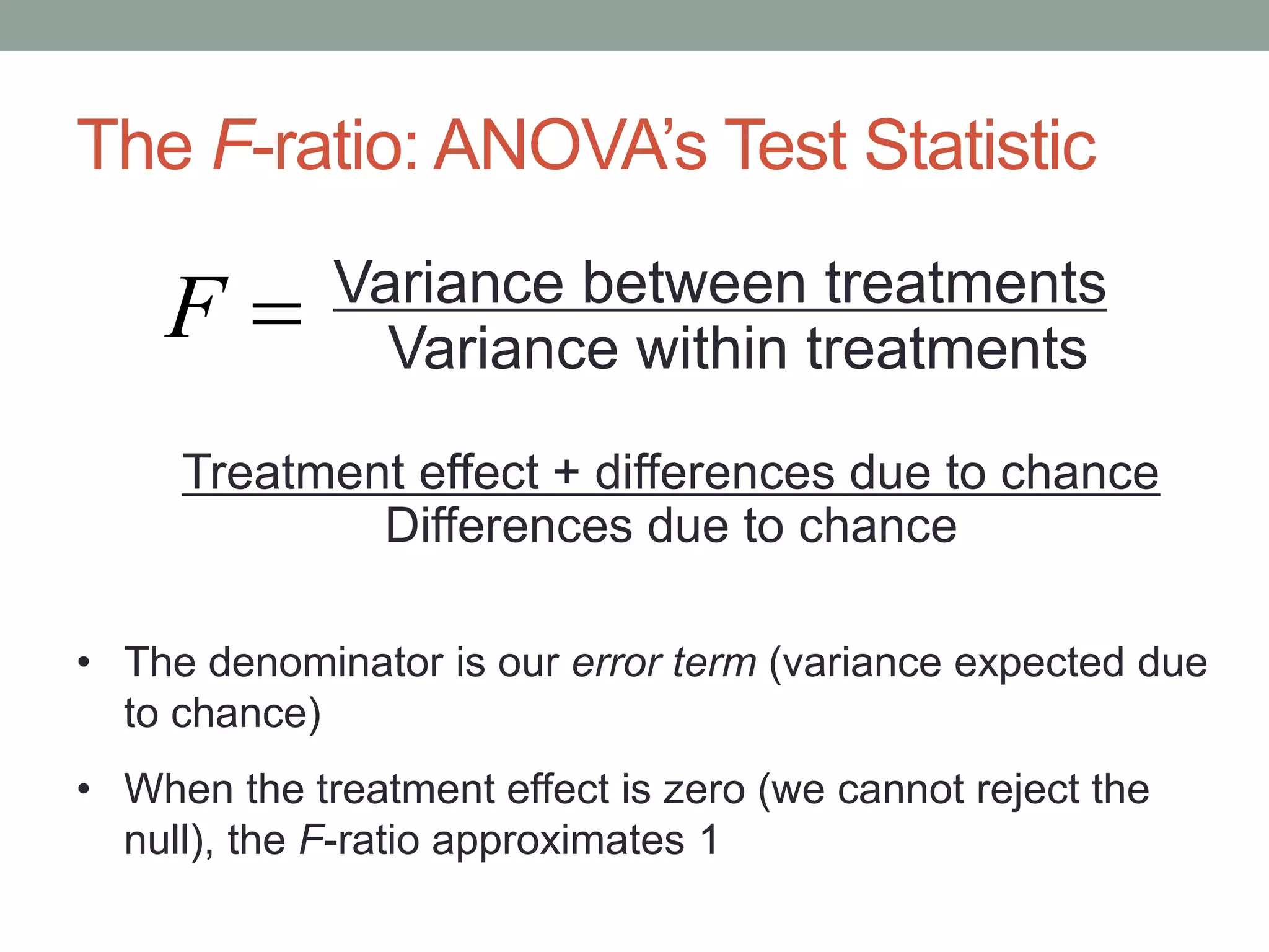
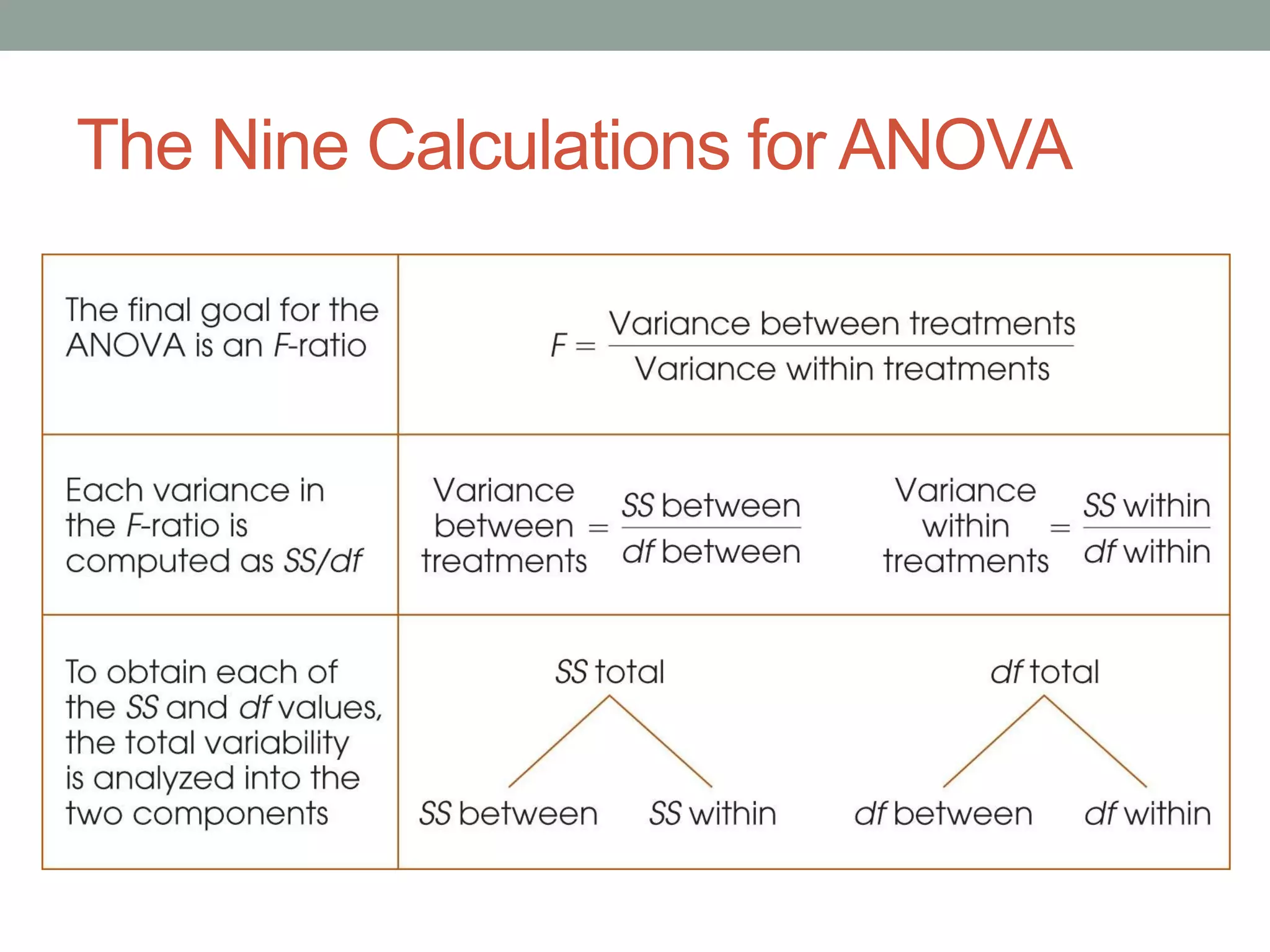
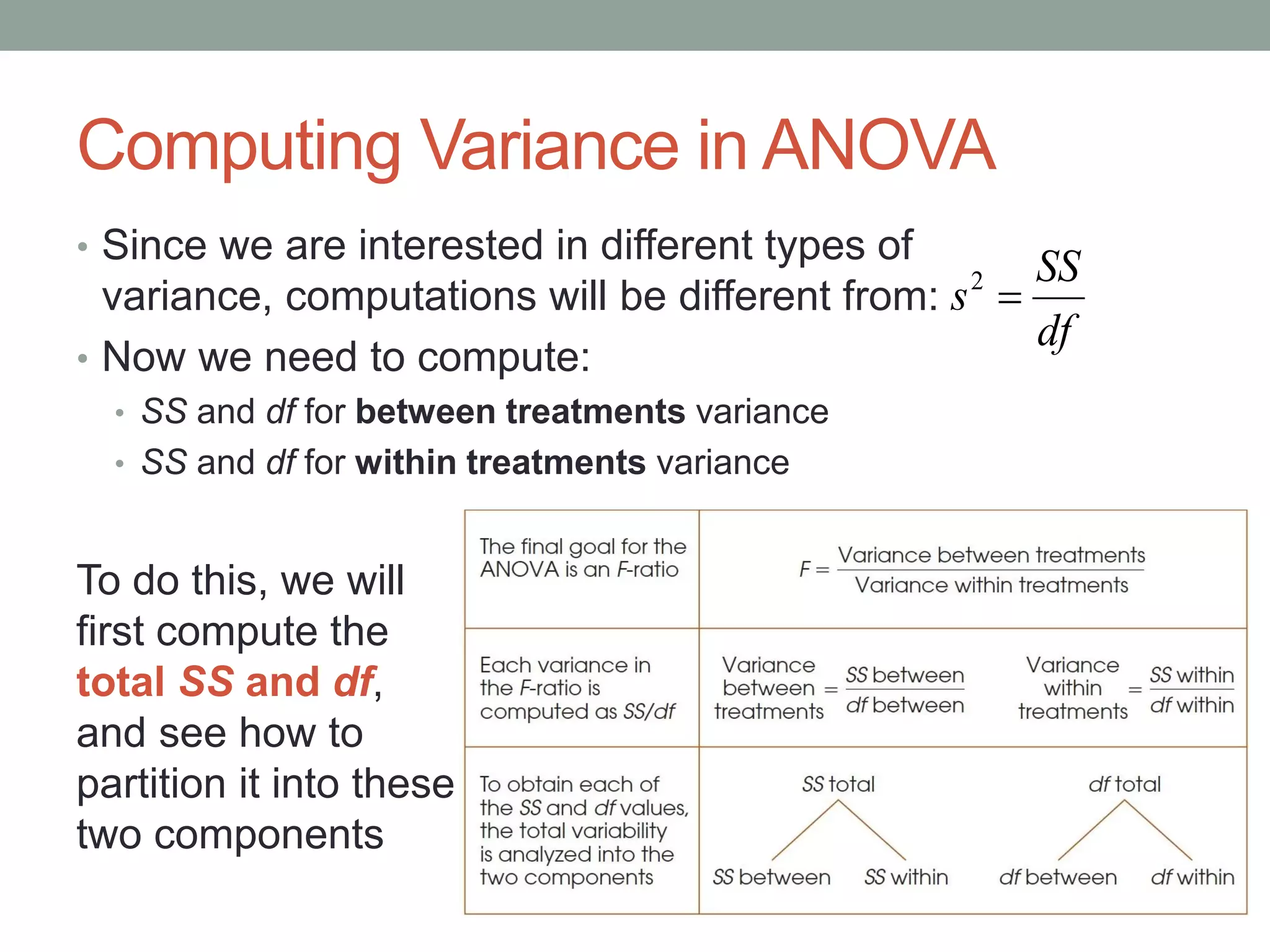
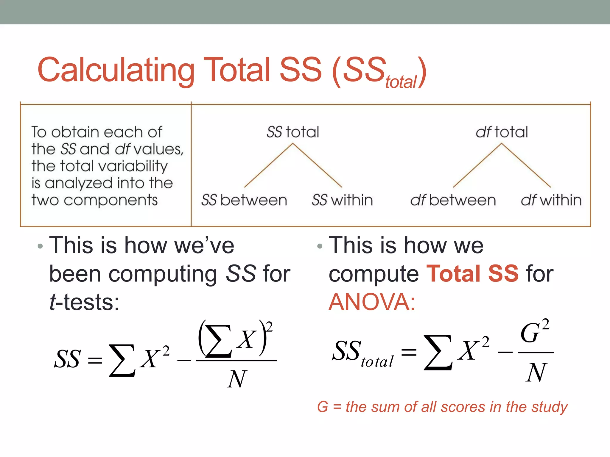
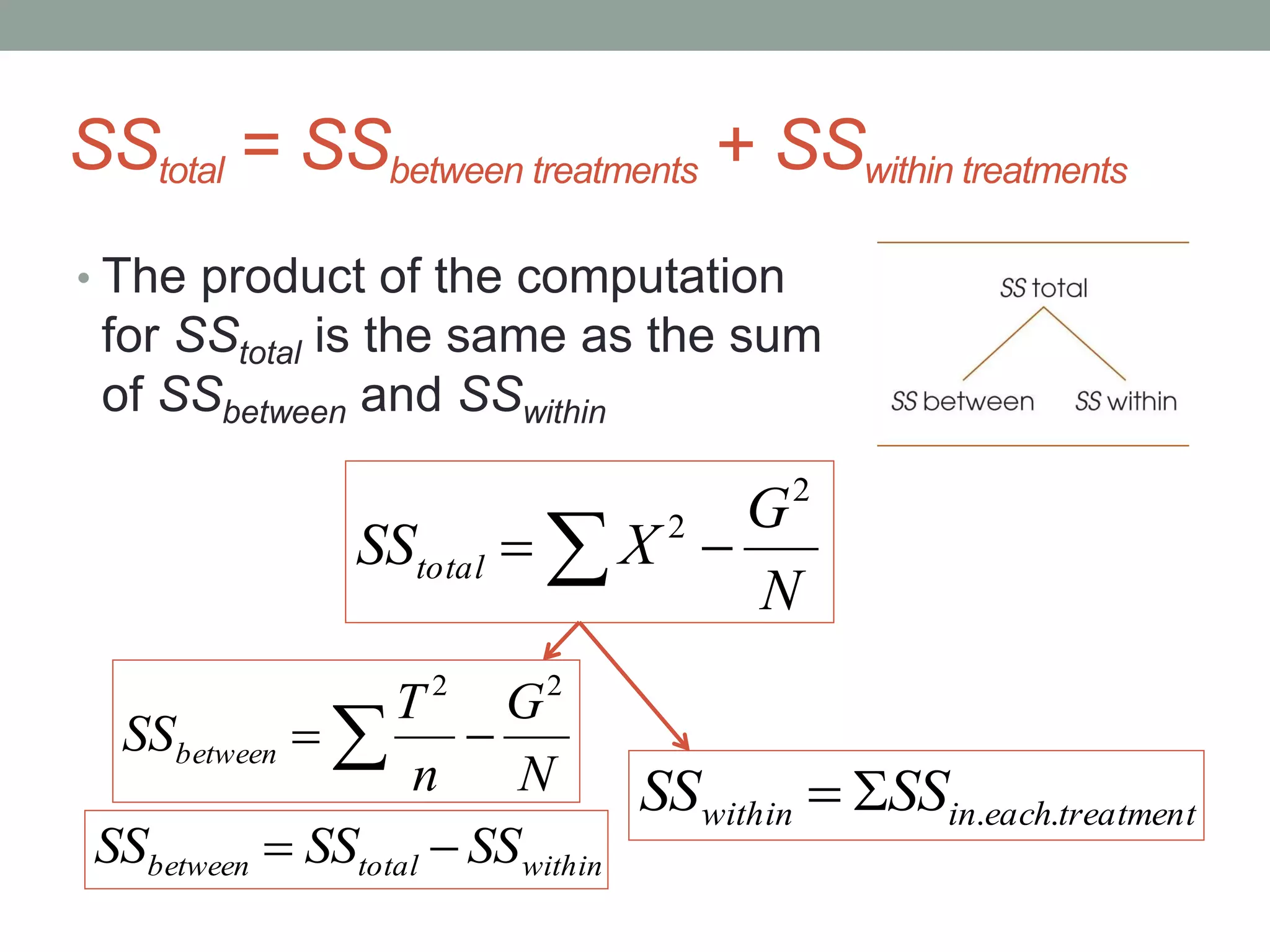
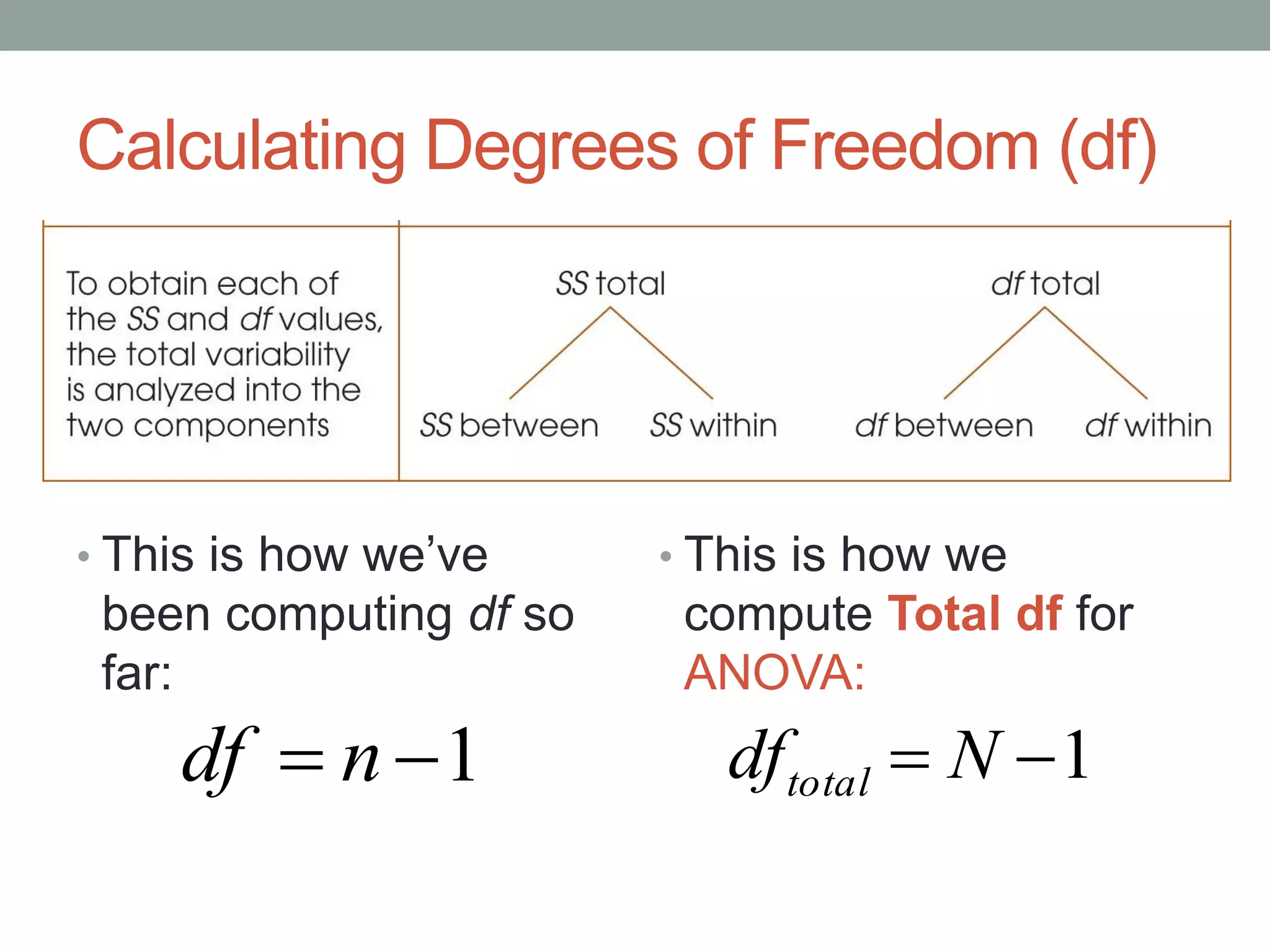
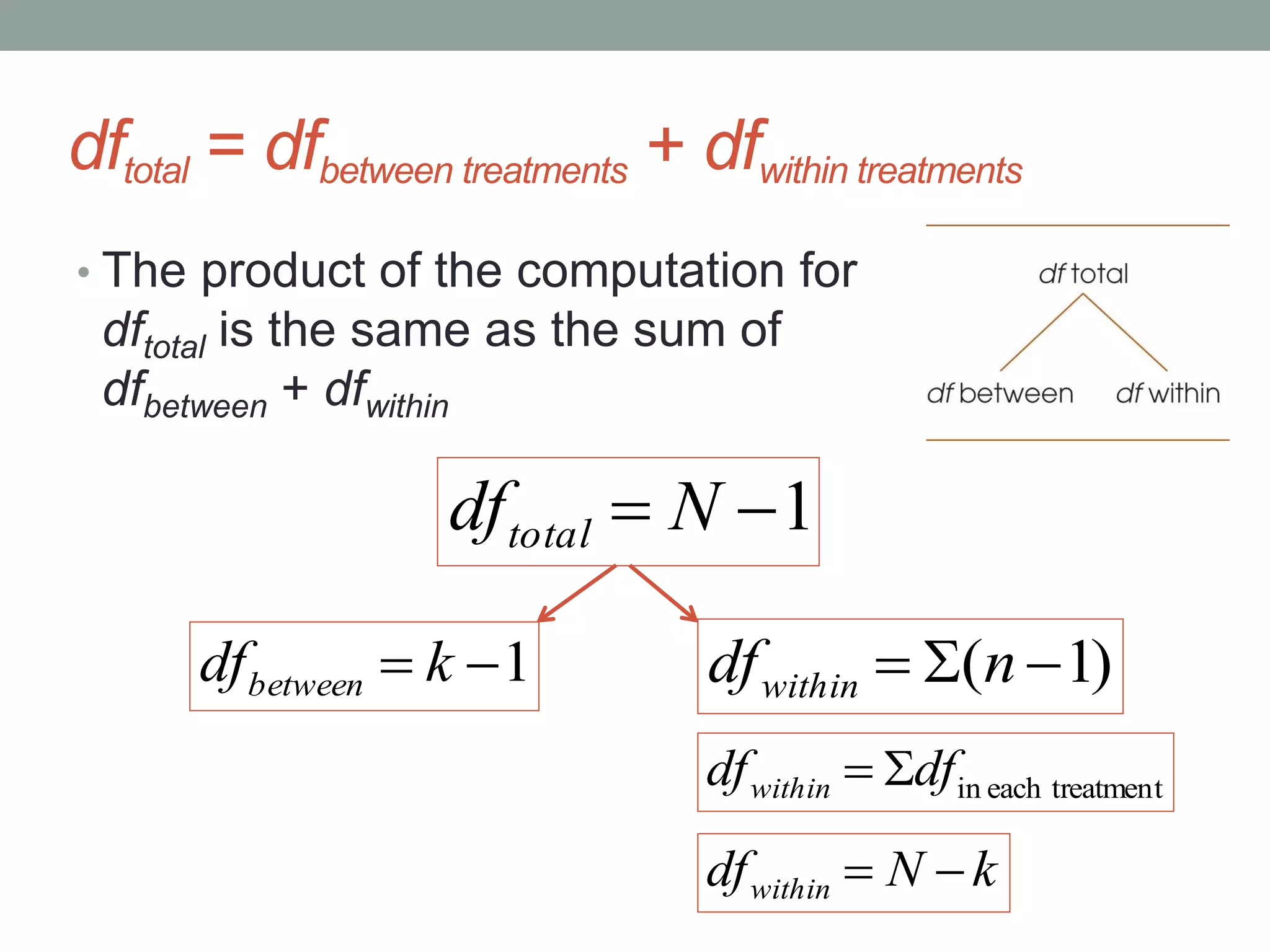
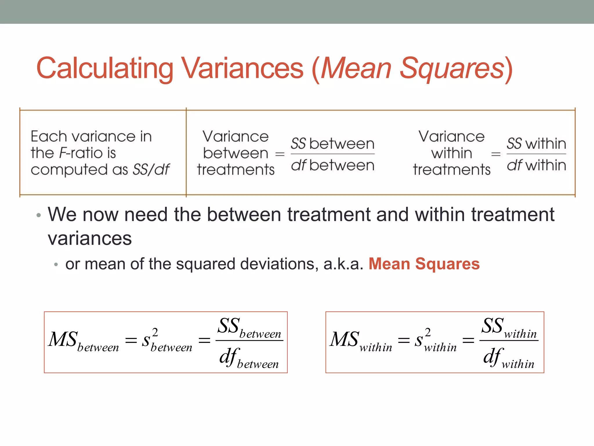
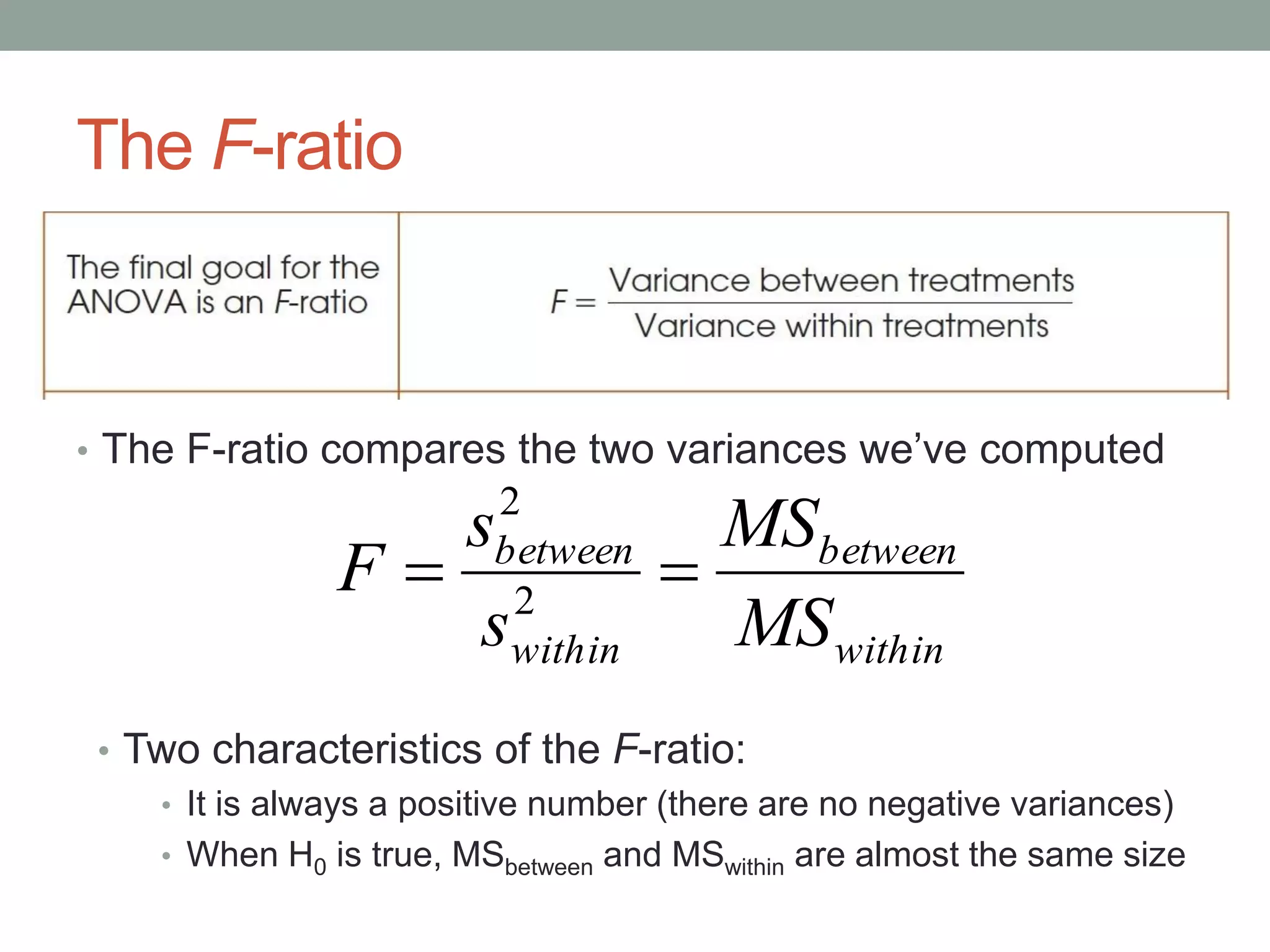
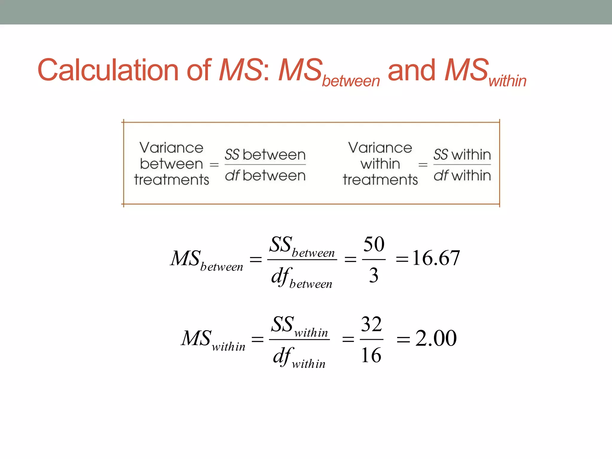
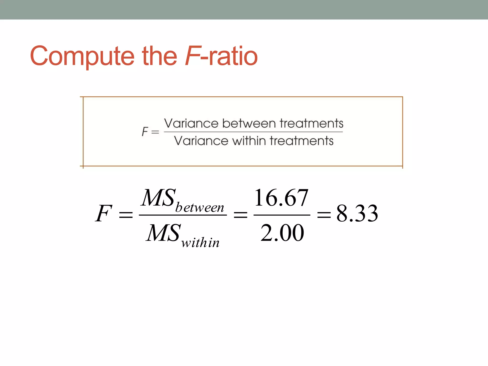
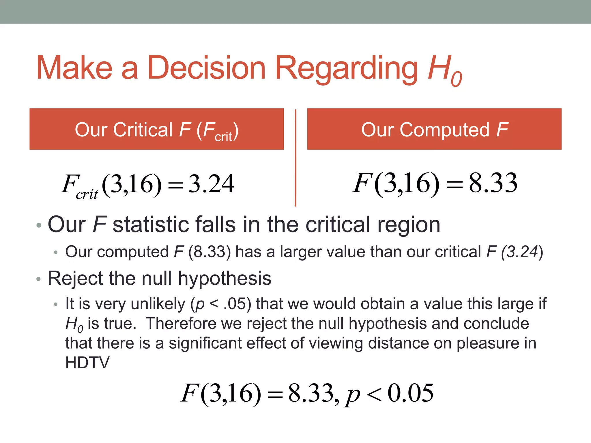
CHAPTER 12
Introduction to
Analysis of Variance
(ANOVA)
ANOVA
What have we learned so far?
z-statistic Tests a claim about a population mean with a
sample mean (and σ is known)
One-sample
t-statistic
Tests a claim about a population mean with a
sample mean (σ unknown)
Independent-
measures
t-statistic
Tests a claim about the difference between two
population means by using two samples and
evaluating their mean difference
Rogers, Kuiper,
& Kirker (1977)
An experiment demonstrating the effect of
levels of processing (superficial to deep) on
memorization of events
• All participants were given a surprise memory test
• They were not told beforehand that they needed to
memorize the words on the list
Treatment 1
Population 1
Treatment 2
Population 2
Treatment 3
Population 3
Treatment 4
Population 4
Superficial
processing
Deep
Processing
Physical
characteristic
Sound
characteristic
Meaning Relation to
Self
How do we evaluate
differences between
4 different means?
Analysis of Variance!
• Tests claims about mean differences between two or
more populations by using two or more samples
• The tested hypothesis is very similar to the independent-
measures t-statistic, but now can be applied when we
have more than two groups
How do we evaluate
differences between
4 different means?
ATypical Example of a Situation
Requiring ANOVA
• t-tests only allow the comparison of 2 means at a time
• This would require 3 separate t-tests with 3 separate α-
levels, which accumulate over a series of tests
• ANOVA allows the evaluation of all three means at once
Terminology in ANOVA
• The variable that designates the groups being compared is called a
factor (e.g., “telephone condition,” “age”)
• The individual conditions or values that make up a factor are called
levels of the factor (e.g., 3 telephone conditions, 3 age groups)
No phone Hands-free Hand-held
Independent Variable:
Telephone conditions
Three treatment
conditions are created
by the researcher
6-yr-olds 8-yr-olds 10-yr-olds
Quasi-Independent
Variable: Age
Non-manipulated variable
used to create groups
Research Designs for ANOVA
• Independent-measures design
• Uses a separate group of participants for each of the treatment
conditions being compared
• Repeated-measures design
• Uses one group of participants for all of the treatment conditions
• Two-factor (or Factorial) design
• To be covered in Chapter 14
Statistical Hypotheses for ANOVA
• All populations have the same mean
(there is no mean difference between any of the groups)
• Telephone condition has no effect on driving performance
held-handfree-handsphoneno0 :  H
The Null
Hypothesis
No phone Hands-free Hand-heldTelephone
conditions
Statistical Hypotheses for ANOVA
No phone Hands-free Hand-heldTelephone
conditions
• At least one of the population means is different from
another (no specific decision which or how they differ)
• Not all treatment conditions are the same, there is a
treatment effect somewhere
The Alternative
Hypothesis
:1H There is at least one mean difference among populations
The Alternative Hypothesis
held-handfree-handsphoneno0 :  H
held-handfree-handsphoneno0 :  H
held-handfree-handsphoneno0 :  H
The Test Statistic for ANOVA
(error)chancebyexpectedDifference
meanssampleobetween twdifferenceObtained
t
The F-ratio
• A ratio of two sample variances
• a.k.a. mean squares, or MS values
• The same basic structure as the independent-measures t
statistic:
obtained mean differences (including treatment effects) MSbetween
F = ────────────────────────────────── = ───────
differences expected by chance (without treatment effects) MSwithin
Why Variance vs. Mean Differences?
However, we can evaluate the variance between these
three means:
A small variance represents small differences between the sample means
When we have
more than two
sample means,
how do you
evaluate a mean
difference?
It’s problematic
624.15
2
247.31
13
3
)4.72(
5.1778
1
2
2






n
SS
s
Type I Errors and Multiple-Hypothesis Tests
Why not just use multiple t-tests?
• Each time we conduct a t-test, we risk a Type I error
• The level of risk for making a Type I error is set by our α-level
• For an IV (telephone conditions) with three levels (none,
hands-free, hand-held), we would need three separate
t-tests
1. None v. hands-free; α = .05
2. None v. hand-held; α = .05
3. Hands-free v. hand-held; α = .05
• Each test compounds the chance of making an experiment-
wide Type I error
With ANOVA, we maintain an α = .05
CHAPTER 12.2
The Logic of ANOVA
The
Logic of
ANOVA
• Three steps:
1. Calculate between-treatments variance
1. Here we see that there is large variance between
sample means
2. Calculate within-treatment variance
1. There is some variability in scores within each
sample
3. Calculate the F-ratio to compare the two
variances
These scores are all
different. Or, in
statistical terms, these
scores are all variable.
Our goal is to measure
the amount of
variability to explain
why the scores are
different
This is Analysis of Variance, people!
Between-Treatments Variance
“Good” variance
• This is the variance we are
interested in
• Differences between samples
• Possible sources of
variance:
• Differences caused by
treatment
• Random chance
• How do participants in
different conditions differ?
Within-Treatments Variance
“Bad” variance
• Variance due to chance
and sampling error
• “Noise”
• How big are the
differences between
individuals when there is
no treatment effect?
• How do participants within
the same condition differ?
A Graphic Illustration
The F-ratio: ANOVA’s Test Statistic
Variance between treatments
Variance within treatments
Treatment effect + differences due to chance
Differences due to chance
F
• The denominator is our error term (variance expected due
to chance)
• When the treatment effect is zero (we cannot reject the
null), the F-ratio approximates 1
CHAPTER 12.3
ANOVA Notation and Formulas
ANOVA
Notation
• k = the number of levels of the factor
• n = the number of scores in each treatment
• N = the total number of scores in the study
• T = the sum of scores (∑X) for a specific treatment
• G = the sum of all scores (∑T) in the study
The textbook authors note that
they have introduced the
notations “T” and “G”
• “T” = “Treatment Total”
• “G” = “Grand Total”
Other sources may use
different notations.
The Nine Calculations for ANOVA
Computing Variance in ANOVA
• Since we are interested in different types of
variance, computations will be different from:
• Now we need to compute:
• SS and df for between treatments variance
• SS and df for within treatments variance
To do this, we will
first compute the
total SS and df,
and see how to
partition it into these
two components
df
SS
s 2
Calculating Total SS (SStotal)
• This is how we’ve
been computing SS for
t-tests:
• This is how we
compute Total SS for
ANOVA:
G = the sum of all scores in the study
 
N
X
XSS
2
2  
N
G
XSStotal
2
2
 
SStotal = SSbetween treatments + SSwithin treatments
• The product of the computation
for SStotal is the same as the sum
of SSbetween and SSwithin
N
G
XSStotal
2
2
 
 
N
G
n
T
SSbetween
22
treatmenteachinwithin SSSS ..
withintotalbetween SSSSSS 
Calculating Degrees of Freedom (df)
• This is how we’ve
been computing df so
far:
• This is how we
compute Total df for
ANOVA:
1 ndf 1 Ndftotal
dftotal = dfbetween treatments + dfwithin treatments
• The product of the computation for
dftotal is the same as the sum of
dfbetween + dfwithin
1 kdfbetween )1(  ndfwithin
menteach treatindfdfwithin 
kNdfwithin 
1 Ndftotal
Calculating Variances (Mean Squares)
• We now need the between treatment and within treatment
variances
• or mean of the squared deviations, a.k.a. Mean Squares
between
between
betweenbetween
df
SS
sMS  2
within
within
withinwithin
df
SS
sMS  2
The F-ratio
• The F-ratio compares the two variances we’ve computed
within
between
within
between
MS
MS
s
s
F  2
2
• Two characteristics of the F-ratio:
• It is always a positive number (there are no negative variances)
• When H0 is true, MSbetween and MSwithin are almost the same size
ANOVA Summary Table
• Comprehensively summarizes all important
elements in the calculation, and allows you to
check your work
Source SS df MS
Between treatments 30 2 15 F = 11.28
Within treatments 16 12 1.33
Total 46 14
CHAPTER 12.4
The Distribution of F-ratios
We have the F-statistic – what now?
• Now we have a test statistic that gives us a ratio of the
differences between treatments to differences attributed to
error
• To evaluate this statistic, we must consider our α-level
and consult the F-distribution table (up next)
• We compare this statistic to some critical value that defines
“unlikely” events in the F-distribution
The F-distribution
• Exact shape will change
with df
• df between (numerator)
• df within (denominator)
• Two characteristics of F:
• It is always a positive
number (there are no
negative variances)
• When H0 is true, MSbetween
and MSwithin are almost the
same size (equal to or
close to 1)
The F Distribution Table (pp. 705-707)
CHAPTER 12.5
Examples of Hypothesis Testing and Effect Size with
ANOVA
Hypothesis Testing Using ANOVA
We have more than 2 groups of data to compare
(independent measures, one-factor)
1. State H0 and H1
2. Set the alpha level and locate the critical region
1. Compute df (total, within, between)
3. Compute the F-ratio
1. Compute SS (total, within, between)
2. Compute MS (between, within)
3. Compute F
4. Make a decision
• Either “reject” or “fail to reject” H0
Example 12.1
• Are there any differences in satisfaction with different
viewing distances of a 42-inch HDTV?
Step 1: State your hypotheses and set α
• There is no effect of viewing distances on ratings of
satisfaction of watching HDTV
43210 :  H
differentismeanstheofoneleastat:1H
• There is an effect of viewing distances on ratings of
satisfaction of watching HDTV
05.0
Step 2: Locate the Critical Region
df for the F-ratio: 3, 16
1 kdfbetween
kNdfwithin 
1 Ndftotal
19120 
314 
16420 
24.3)16,3( critF
Step 3: Compute the F-ratio
• Remember this guideline - we start from the bottom up
Analyze the SS to get SSbetween and SSwithin
• SStotal is the SS for the total set
of N = 20 scores
N
G
XSStotal
2
2
 
withintotalbetween SSSSSS 
treatmenteachinwithin SSSS ..
20
60
262
2

20
360
262 82180262 
• SSwithin combines the SS values from each treatment condition
3261088 
• SSbetween since we already computed Sstotal and SSwithin::
503282 
Next we calculate MS
Calculation of MS: MSbetween and MSwithin
between
between
between
df
SS
MS 
within
within
within
df
SS
MS 
3
50
 67.16
16
32
 00.2
Compute the F-ratio
33.8
00.2
67.16

within
between
MS
MS
F
The Summary Table for Example 12.1
Source SS Df MS
Between
treatments
50 3 16.67 F = 8.33
Within
treatments
32 16 2.00
Total 82 19
Make a Decision Regarding H0
Our Critical F (Fcrit)
• Our F statistic falls in the critical region
• Our computed F (8.33) has a larger value than our critical F (3.24)
• Reject the null hypothesis
• It is very unlikely (p < .05) that we would obtain a value this large if
H0 is true. Therefore we reject the null hypothesis and conclude
that there is a significant effect of viewing distance on pleasure in
HDTV
Our Computed F
24.3)16,3( critF 33.8)16,3( F
05.0,33.8)16,3(  pF
What if there are unequal sample sizes in
my different groups?
• Sample variance contributes to our estimate of
error in the denominator
• What did we do when we had unequal sample
sizes with the independent-measures t-test?
Pooled variance: we do the same with ANOVA
k
k
within
within
within
dfdfdf
SSSSSS
df
SS
MS



...
...
21
21
CHAPTER 12.6
Post Hoc Tests
Measuring effect size for ANOVA
A significant difference indicates our difference is
larger than expected by chance, but does not tell
us how large this difference is
η² = the percentage of variance accounted for
total
between
SS
SS
2

What if I have a significant F-ratio?
Reject the null hypothesis. There is a significant
difference somewhere between at least two of the
groups (not all groups are equal)
But I don’t know where the difference is
If I have three groups:
Group A could be different than B
or group B from C
or group A from C.
So, if there is a significant F-ratio,
more tests must be done
to find which groups are different
Post hoc tests
Additional hypothesis tests that are done after an
ANOVA results in a significant F-ratio to determine
exactly which mean differences are significant and
which are not
• Finds where the significant differences are
• Developed to control the experiment-wise error
rate
Tukey’s Honestly Significant Difference (HSD)
Scheffé Test
Tukey’s HSD
Tells us the minimum difference between treatment
means that is necessary for significance
q: “Studentized range statistic” found in Table B.5
Must know k, df within treatments, and set α
n: number of scores in each treatment (requires
equal sample sizes in all groups)
n
MS
qHSD within

Scheffé Test
• More conservative than Tukey’s HSD
• Uses the ANOVA formula, but only compares two
groups at a time
• The denominator will remain the same as the overall
ANOVA (MS within), but the numerator will be
recalculated based only on the two groups in question
Start with the two groups that have the largest
mean difference, and work down until you have a
non-significant result
For the Scheffé Test:
• SS between treatments (and MS between) is recalculated
using only the two groups in question
• MS within remains the same from the overall ANOVA test
within
between
between
between
between
between
MS
MS
F
df
SS
MS
N
G
n
T
SS


 
22
Use the same critical value
as the overall ANOVA,
even though we now
only are comparing two
groups
Additional ANOVA steps:
8. Compute η² if necessary
9. Compute post-hoc tests if necessary to determine
where significant differences between groups are
located
10. Make some sort of overall statement summarizing all
the results of your study

Analysis of Variance

  • 1.
    CHAPTER 12 Introduction to Analysisof Variance (ANOVA) ANOVA
  • 2.
    What have welearned so far? z-statistic Tests a claim about a population mean with a sample mean (and σ is known) One-sample t-statistic Tests a claim about a population mean with a sample mean (σ unknown) Independent- measures t-statistic Tests a claim about the difference between two population means by using two samples and evaluating their mean difference
  • 3.
    Rogers, Kuiper, & Kirker(1977) An experiment demonstrating the effect of levels of processing (superficial to deep) on memorization of events • All participants were given a surprise memory test • They were not told beforehand that they needed to memorize the words on the list Treatment 1 Population 1 Treatment 2 Population 2 Treatment 3 Population 3 Treatment 4 Population 4 Superficial processing Deep Processing Physical characteristic Sound characteristic Meaning Relation to Self How do we evaluate differences between 4 different means?
  • 4.
    Analysis of Variance! •Tests claims about mean differences between two or more populations by using two or more samples • The tested hypothesis is very similar to the independent- measures t-statistic, but now can be applied when we have more than two groups How do we evaluate differences between 4 different means?
  • 5.
    ATypical Example ofa Situation Requiring ANOVA • t-tests only allow the comparison of 2 means at a time • This would require 3 separate t-tests with 3 separate α- levels, which accumulate over a series of tests • ANOVA allows the evaluation of all three means at once
  • 6.
    Terminology in ANOVA •The variable that designates the groups being compared is called a factor (e.g., “telephone condition,” “age”) • The individual conditions or values that make up a factor are called levels of the factor (e.g., 3 telephone conditions, 3 age groups) No phone Hands-free Hand-held Independent Variable: Telephone conditions Three treatment conditions are created by the researcher 6-yr-olds 8-yr-olds 10-yr-olds Quasi-Independent Variable: Age Non-manipulated variable used to create groups
  • 7.
    Research Designs forANOVA • Independent-measures design • Uses a separate group of participants for each of the treatment conditions being compared • Repeated-measures design • Uses one group of participants for all of the treatment conditions • Two-factor (or Factorial) design • To be covered in Chapter 14
  • 8.
    Statistical Hypotheses forANOVA • All populations have the same mean (there is no mean difference between any of the groups) • Telephone condition has no effect on driving performance held-handfree-handsphoneno0 :  H The Null Hypothesis No phone Hands-free Hand-heldTelephone conditions
  • 9.
    Statistical Hypotheses forANOVA No phone Hands-free Hand-heldTelephone conditions • At least one of the population means is different from another (no specific decision which or how they differ) • Not all treatment conditions are the same, there is a treatment effect somewhere The Alternative Hypothesis :1H There is at least one mean difference among populations
  • 10.
    The Alternative Hypothesis held-handfree-handsphoneno0:  H held-handfree-handsphoneno0 :  H held-handfree-handsphoneno0 :  H
  • 11.
    The Test Statisticfor ANOVA (error)chancebyexpectedDifference meanssampleobetween twdifferenceObtained t The F-ratio • A ratio of two sample variances • a.k.a. mean squares, or MS values • The same basic structure as the independent-measures t statistic: obtained mean differences (including treatment effects) MSbetween F = ────────────────────────────────── = ─────── differences expected by chance (without treatment effects) MSwithin
  • 12.
    Why Variance vs.Mean Differences? However, we can evaluate the variance between these three means: A small variance represents small differences between the sample means When we have more than two sample means, how do you evaluate a mean difference? It’s problematic 624.15 2 247.31 13 3 )4.72( 5.1778 1 2 2       n SS s
  • 13.
    Type I Errorsand Multiple-Hypothesis Tests Why not just use multiple t-tests? • Each time we conduct a t-test, we risk a Type I error • The level of risk for making a Type I error is set by our α-level • For an IV (telephone conditions) with three levels (none, hands-free, hand-held), we would need three separate t-tests 1. None v. hands-free; α = .05 2. None v. hand-held; α = .05 3. Hands-free v. hand-held; α = .05 • Each test compounds the chance of making an experiment- wide Type I error With ANOVA, we maintain an α = .05
  • 14.
  • 15.
    The Logic of ANOVA • Threesteps: 1. Calculate between-treatments variance 1. Here we see that there is large variance between sample means 2. Calculate within-treatment variance 1. There is some variability in scores within each sample 3. Calculate the F-ratio to compare the two variances These scores are all different. Or, in statistical terms, these scores are all variable. Our goal is to measure the amount of variability to explain why the scores are different
  • 16.
    This is Analysisof Variance, people! Between-Treatments Variance “Good” variance • This is the variance we are interested in • Differences between samples • Possible sources of variance: • Differences caused by treatment • Random chance • How do participants in different conditions differ? Within-Treatments Variance “Bad” variance • Variance due to chance and sampling error • “Noise” • How big are the differences between individuals when there is no treatment effect? • How do participants within the same condition differ?
  • 17.
  • 18.
    The F-ratio: ANOVA’sTest Statistic Variance between treatments Variance within treatments Treatment effect + differences due to chance Differences due to chance F • The denominator is our error term (variance expected due to chance) • When the treatment effect is zero (we cannot reject the null), the F-ratio approximates 1
  • 19.
  • 20.
    ANOVA Notation • k =the number of levels of the factor • n = the number of scores in each treatment • N = the total number of scores in the study • T = the sum of scores (∑X) for a specific treatment • G = the sum of all scores (∑T) in the study The textbook authors note that they have introduced the notations “T” and “G” • “T” = “Treatment Total” • “G” = “Grand Total” Other sources may use different notations.
  • 21.
  • 22.
    Computing Variance inANOVA • Since we are interested in different types of variance, computations will be different from: • Now we need to compute: • SS and df for between treatments variance • SS and df for within treatments variance To do this, we will first compute the total SS and df, and see how to partition it into these two components df SS s 2
  • 23.
    Calculating Total SS(SStotal) • This is how we’ve been computing SS for t-tests: • This is how we compute Total SS for ANOVA: G = the sum of all scores in the study   N X XSS 2 2   N G XSStotal 2 2  
  • 24.
    SStotal = SSbetweentreatments + SSwithin treatments • The product of the computation for SStotal is the same as the sum of SSbetween and SSwithin N G XSStotal 2 2     N G n T SSbetween 22 treatmenteachinwithin SSSS .. withintotalbetween SSSSSS 
  • 25.
    Calculating Degrees ofFreedom (df) • This is how we’ve been computing df so far: • This is how we compute Total df for ANOVA: 1 ndf 1 Ndftotal
  • 26.
    dftotal = dfbetweentreatments + dfwithin treatments • The product of the computation for dftotal is the same as the sum of dfbetween + dfwithin 1 kdfbetween )1(  ndfwithin menteach treatindfdfwithin  kNdfwithin  1 Ndftotal
  • 27.
    Calculating Variances (MeanSquares) • We now need the between treatment and within treatment variances • or mean of the squared deviations, a.k.a. Mean Squares between between betweenbetween df SS sMS  2 within within withinwithin df SS sMS  2
  • 28.
    The F-ratio • TheF-ratio compares the two variances we’ve computed within between within between MS MS s s F  2 2 • Two characteristics of the F-ratio: • It is always a positive number (there are no negative variances) • When H0 is true, MSbetween and MSwithin are almost the same size
  • 29.
    ANOVA Summary Table •Comprehensively summarizes all important elements in the calculation, and allows you to check your work Source SS df MS Between treatments 30 2 15 F = 11.28 Within treatments 16 12 1.33 Total 46 14
  • 30.
  • 31.
    We have theF-statistic – what now? • Now we have a test statistic that gives us a ratio of the differences between treatments to differences attributed to error • To evaluate this statistic, we must consider our α-level and consult the F-distribution table (up next) • We compare this statistic to some critical value that defines “unlikely” events in the F-distribution
  • 32.
    The F-distribution • Exactshape will change with df • df between (numerator) • df within (denominator) • Two characteristics of F: • It is always a positive number (there are no negative variances) • When H0 is true, MSbetween and MSwithin are almost the same size (equal to or close to 1)
  • 33.
    The F DistributionTable (pp. 705-707)
  • 34.
    CHAPTER 12.5 Examples ofHypothesis Testing and Effect Size with ANOVA
  • 35.
    Hypothesis Testing UsingANOVA We have more than 2 groups of data to compare (independent measures, one-factor) 1. State H0 and H1 2. Set the alpha level and locate the critical region 1. Compute df (total, within, between) 3. Compute the F-ratio 1. Compute SS (total, within, between) 2. Compute MS (between, within) 3. Compute F 4. Make a decision • Either “reject” or “fail to reject” H0
  • 36.
    Example 12.1 • Arethere any differences in satisfaction with different viewing distances of a 42-inch HDTV?
  • 37.
    Step 1: Stateyour hypotheses and set α • There is no effect of viewing distances on ratings of satisfaction of watching HDTV 43210 :  H differentismeanstheofoneleastat:1H • There is an effect of viewing distances on ratings of satisfaction of watching HDTV 05.0
  • 38.
    Step 2: Locatethe Critical Region df for the F-ratio: 3, 16 1 kdfbetween kNdfwithin  1 Ndftotal 19120  314  16420  24.3)16,3( critF
  • 39.
    Step 3: Computethe F-ratio • Remember this guideline - we start from the bottom up
  • 40.
    Analyze the SSto get SSbetween and SSwithin • SStotal is the SS for the total set of N = 20 scores N G XSStotal 2 2   withintotalbetween SSSSSS  treatmenteachinwithin SSSS .. 20 60 262 2  20 360 262 82180262  • SSwithin combines the SS values from each treatment condition 3261088  • SSbetween since we already computed Sstotal and SSwithin:: 503282 
  • 41.
  • 42.
    Calculation of MS:MSbetween and MSwithin between between between df SS MS  within within within df SS MS  3 50  67.16 16 32  00.2
  • 43.
  • 44.
    The Summary Tablefor Example 12.1 Source SS Df MS Between treatments 50 3 16.67 F = 8.33 Within treatments 32 16 2.00 Total 82 19
  • 45.
    Make a DecisionRegarding H0 Our Critical F (Fcrit) • Our F statistic falls in the critical region • Our computed F (8.33) has a larger value than our critical F (3.24) • Reject the null hypothesis • It is very unlikely (p < .05) that we would obtain a value this large if H0 is true. Therefore we reject the null hypothesis and conclude that there is a significant effect of viewing distance on pleasure in HDTV Our Computed F 24.3)16,3( critF 33.8)16,3( F 05.0,33.8)16,3(  pF
  • 46.
    What if thereare unequal sample sizes in my different groups? • Sample variance contributes to our estimate of error in the denominator • What did we do when we had unequal sample sizes with the independent-measures t-test? Pooled variance: we do the same with ANOVA k k within within within dfdfdf SSSSSS df SS MS    ... ... 21 21
  • 47.
  • 48.
    Measuring effect sizefor ANOVA A significant difference indicates our difference is larger than expected by chance, but does not tell us how large this difference is η² = the percentage of variance accounted for total between SS SS 2 
  • 49.
    What if Ihave a significant F-ratio? Reject the null hypothesis. There is a significant difference somewhere between at least two of the groups (not all groups are equal) But I don’t know where the difference is If I have three groups: Group A could be different than B or group B from C or group A from C. So, if there is a significant F-ratio, more tests must be done to find which groups are different
  • 50.
    Post hoc tests Additionalhypothesis tests that are done after an ANOVA results in a significant F-ratio to determine exactly which mean differences are significant and which are not • Finds where the significant differences are • Developed to control the experiment-wise error rate Tukey’s Honestly Significant Difference (HSD) Scheffé Test
  • 51.
    Tukey’s HSD Tells usthe minimum difference between treatment means that is necessary for significance q: “Studentized range statistic” found in Table B.5 Must know k, df within treatments, and set α n: number of scores in each treatment (requires equal sample sizes in all groups) n MS qHSD within 
  • 52.
    Scheffé Test • Moreconservative than Tukey’s HSD • Uses the ANOVA formula, but only compares two groups at a time • The denominator will remain the same as the overall ANOVA (MS within), but the numerator will be recalculated based only on the two groups in question Start with the two groups that have the largest mean difference, and work down until you have a non-significant result
  • 53.
    For the SchefféTest: • SS between treatments (and MS between) is recalculated using only the two groups in question • MS within remains the same from the overall ANOVA test within between between between between between MS MS F df SS MS N G n T SS     22 Use the same critical value as the overall ANOVA, even though we now only are comparing two groups
  • 54.
    Additional ANOVA steps: 8.Compute η² if necessary 9. Compute post-hoc tests if necessary to determine where significant differences between groups are located 10. Make some sort of overall statement summarizing all the results of your study