This document provides an overview of fractal geometry. It begins with an abstract that outlines how fractal patterns found in nature will be used to introduce the concept of fractals. It then provides a brief history of fractals, covering mathematicians like Georg Cantor and Benoit Mandelbrot who contributed to the discovery and study of fractals. The document goes on to examine key properties of fractals in depth, including recursion, self-similarity, iteration, and fractal dimension. It also provides examples of well-known fractals like the Sierpinski triangle and Mandelbrot set to illustrate these properties.
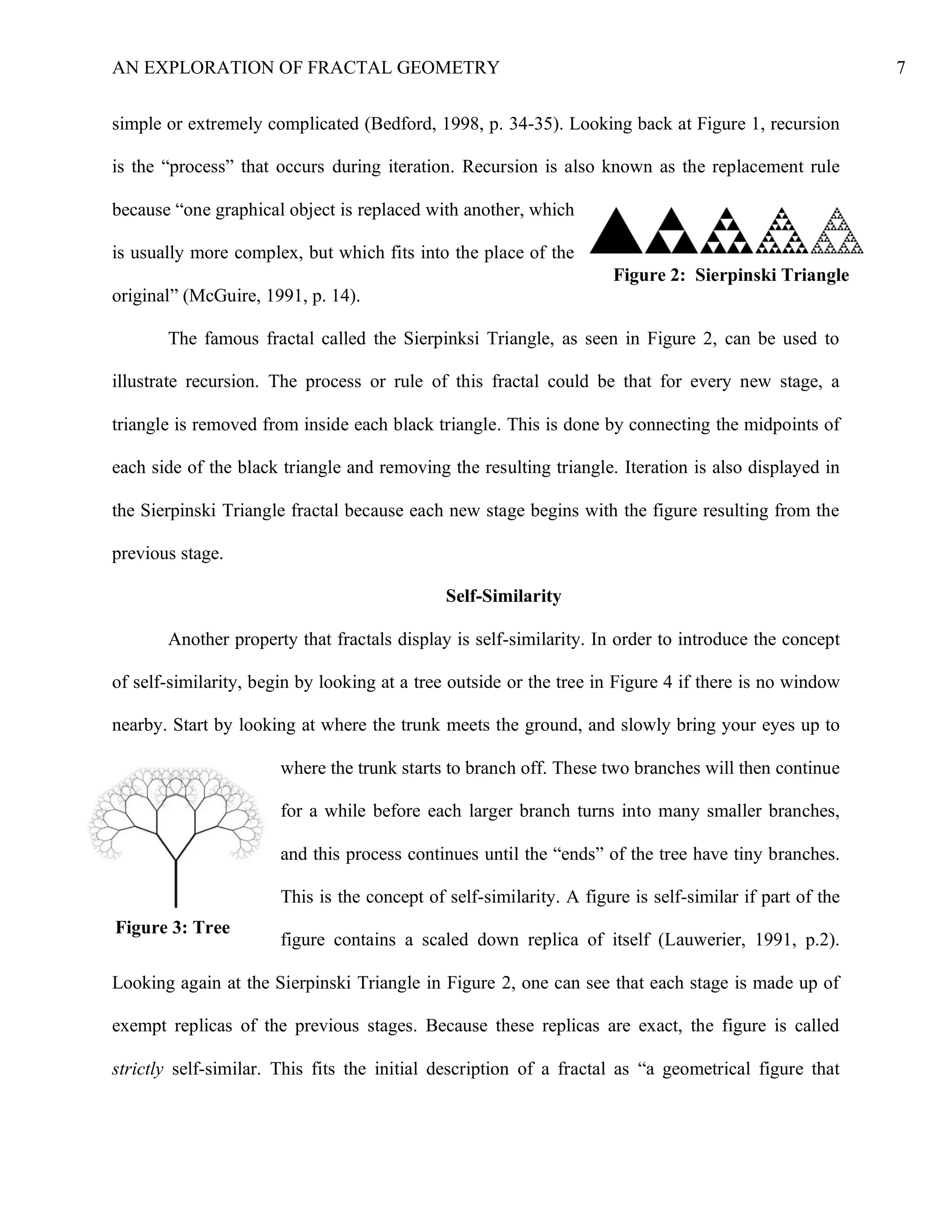
![AN EXPLORATION OF FRACTAL GEOMETRY 11
also have a dimension between 2 and 3 or between 0 and 1 (McGuire, p. 14). For example, if a
fractal surface has a dimension of 2.3 it would mean that it acts like a two-dimensional object
(such as a circle) but it is defined in a three-dimensional space. Consequently, fractal dimensions
such as these “are important because they can be defined in connection with real-world data, and
they can be measured approximately by means of experiments” (Barnsley, 1988, p. 172). What
are some factors than can alter or affect the fractal dimension? When using Mandelbrot’s ruler
method, something that will ultimately affect the dimensional result is the starting point which
one begins to measure the boundary (Landini, 2010, p. 6-7).
The Cantor Set
Now that the concepts of iteration, recursion, self-similarity, and fractal dimension have been
examined in depth, they will be examined against three famous fractals: the Cantor Set, the Koch
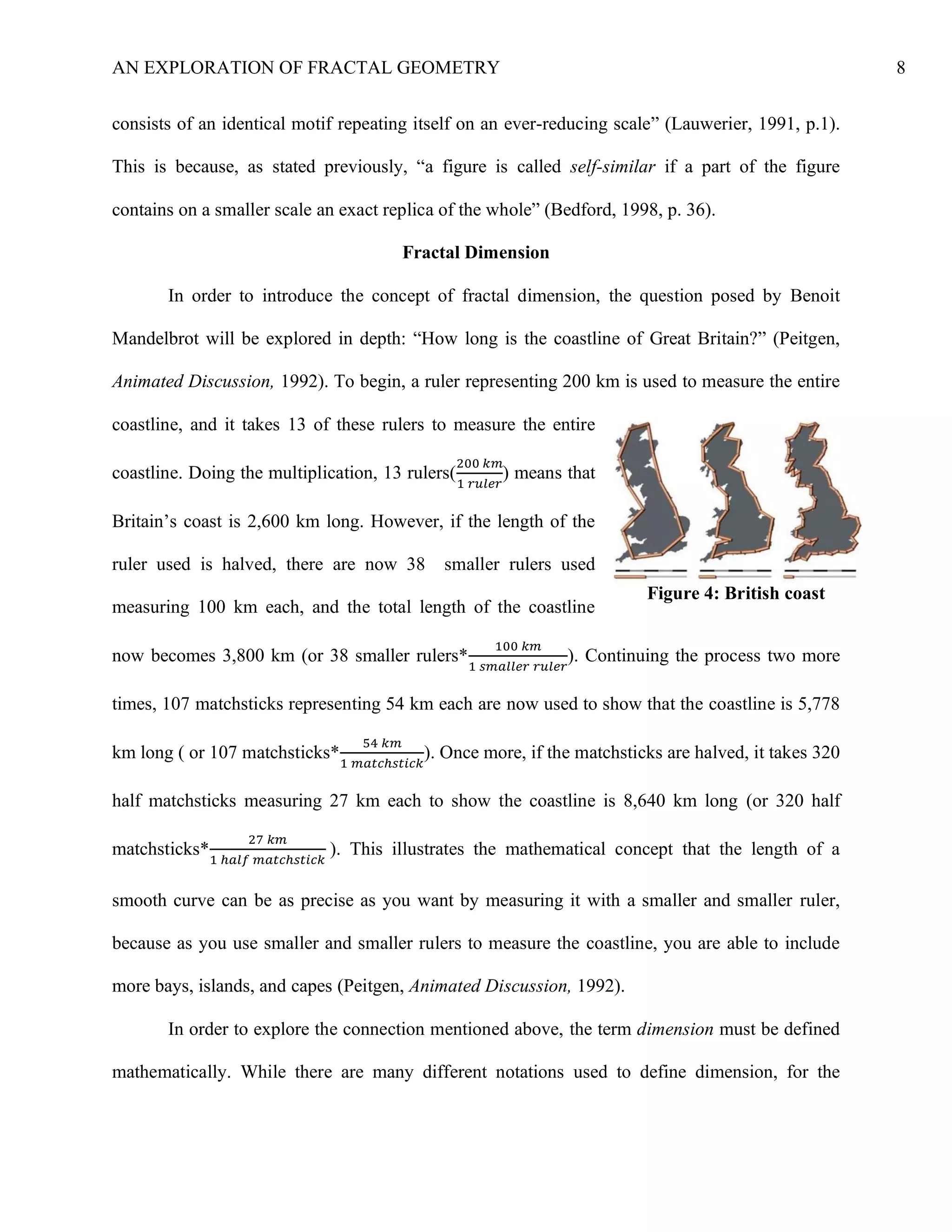
Curve, and the Julia Set. Firstly, the Cantor Set as seen in Figure 7 will be analyzed (Bedford,
1998, p. 47). The German mathematician Georg Cantor (1845-1918) contributed to mathematics
proving that irrational numbers are useful and have a
“logical place” in mathematics, and he is also one of the
main contributors of set theory (Lauwerier, 1991, p. 15).
As seen in Figure 7, the Cantor sets initial stage begins
with a line segment with a length of one, or representing
the interval [0, 1]. In Stage 1, one must “remove the middle third from [0, 1], but not the
numbers 1/3 and 2/3,” so what remains in Stage 1 are “two intervals [0, 1/3] and [2/3, 1] of
length 1/3 each” (Peitgen, Part One, 1992, p. 80). If you do this same process again, you are left
with the union of “four intervals: [0, 1/9] U [2/9, 1/3] U [2/3, 7/9] U [8/9, 1]” as seen in Stage 2
of Figure 7 (Bedford, 1998, p. 46). As you can see from Figure 7, after each iteration the
Figure 7: The Cantor Set](https://image.slidesharecdn.com/anexplorationoffractalgeometry-200429210906/75/An-Exploration-of-Fractal-Geometry-11-2048.jpg)
![AN EXPLORATION OF FRACTAL GEOMETRY 21
References
Barnsley, M. (1988). Fractals Everywhere. United States of America: Academic Press, Inc.
Bedford, C.W. (1998). Introduction to Fractals and Chaos: Mathematics and Meaning.
Andover, MA: Venture Publishing.
(n.d.) Untitled (British Coastline Image). [Photograph]. Retrieved from: https://upload.
wikimedia.org/wikipedia/commons/2/20/Britain-fractal-coastline-combined.jpg.
Gleick, James. (1987). Chaos: Making a New Science. Harrisonburg, VA: R.R. Donnelley &
Sons Co.
Gowers, T. (Ed.) Barrow-Green, J. & Leader, I. (Assoc. eds.). (2008). The Princeton Companion
to Mathematics. Princeton, NJ: Princeton University Press.
Landini, G. (2010). Fractals in microscopy. Journal of Microscopy, 241(1), 1-8.
doi: 10.111/j.1365-2818.2010.03454.x
Lauwerier, H. A. (1991). Fractals: Endlessly Repeated Geometrical Figures. Princeton, NJ:
Princeton University Press.
Mandelbrot, Benoit B. (1977). The Fractal Geometry of Nature. New York: W.H. Freeman and
Company.
McGuire, Michael. (1991). An Eye For Fractals. United States of America: Addison-Wesley
Publishing Co., Inc.
Morphology [Def. 1]. (n.d.). Merriam-Webster Online. In Merriam-Webster. Retrieved
December 13, 2015, from http://www.merriam-webster.com/dictionary/morphology
Parasher, R. (2008). Fractal Dimension: Measuring Infinite Complexity. Pi in The Sky, (12), 3-5.
Peitgen, H.O., Jurgens, H., Saupe, D., Maletsky, E., Perciante, T., & Yunker, L. (1992). Fractals
for the Classroom: Part One Introduction to Fractals and Chaos. Rensselaer, NY:
Springer-Verlag New York, Inc.](https://image.slidesharecdn.com/anexplorationoffractalgeometry-200429210906/75/An-Exploration-of-Fractal-Geometry-21-2048.jpg)
![AN EXPLORATION OF FRACTAL GEOMETRY 22
Peitgen, H.O., Jurgens, H., Saupe, D., & Zahlten C. (Producers). (1990). Fractals: An Animated
Discussion [VHS]. New York: W.H. Freeman and Company.
Strzyzewski, F. [Florian Strzyżewski]. (2008, May 3). More about Julia Set Fractal - part 1 of 3.
[Video File]. Retreived from: https://www.youtube.com/watch?v=RAgR_KVWtcg&
index=2&list=PLymzxCT1I9d3cmOQgZWwjff6jd0uEW0kk.](https://image.slidesharecdn.com/anexplorationoffractalgeometry-200429210906/75/An-Exploration-of-Fractal-Geometry-22-2048.jpg)