AN EOQ MODEL FOR TIME DETERIORATING ITEMS WITH INFINITE & FINITE PRODUCTION RATE WITH SHORTAGE AND COMPLETE BACKLOGGING

Operations Research and Applications : An International Journal (ORAJ), Vol.2, No.4, November 2015
DOI : 10.5121/oraj.2015.2403 31
AN EOQ MODEL FOR TIME DETERIORATING
ITEMS WITH INFINITE & FINITE
PRODUCTION RATE WITH SHORTAGE AND
COMPLETE BACKLOGGING
M. Vijayashree* and R. Uthayakumar
Department of Mathematics,
The Gandhigram Rural Institute – Deemed University,
Gandhigram - 624 302. Dindigul, Tamil Nadu, India.
ABSTRACT
This manuscript deals in developing an EOQ model for time deteriorating items and allowing shortages in
the inventory. These shortages are considered to be completely backlogged. We have held that the
production rate is finite and infinite. In this manuscript, we developed EOQ models for perishable products
which consider continuous deterioration of a utility product and introduce an exponential penalty cost and
linear penalty cost function. The theoretical expressions are obtained for optimum cycle time and optimum
order quantity. The significant centre of our paper is to build up the EOQ model for time-deteriorating
items utilizing penalty cost with finite and infinite production rate. The mathematical solution of the model
has been done to obtain the optimal solution of the problem. The result is demonstrated with the help of
mathematical example. To conclude, sensitivity study is carried out with respect to the key parameters and
some managerial implications are also included. All the theoretical developments are numerically
justified.
KEYWORDS
Inventory, Time deteriorating items, Shortage, Penalty cost.
Subject Classification Code: 90B05
*Corresponding author Tel.: +91-451-2452371, Fax: 91-451-2453071
1. INTRODUCTION
The deterioration of goods is a realistic phenomenon in many inventory systems. The controlling
and regulating of deteriorating items is a measure problem in any inventory system. Certain
products like food stuff, pharmaceuticals, chemicals, volatile liquid, blood and etcetera
deteriorate during their normal storage period. Hence while developing an optimal inventory
policy for such products; the loss of inventory due to deterioration cannot be ignored. The
researchers have continuously modified the deteriorating inventory models so as to become more
practicable and realistic.

32
The majority of the writing on stock control and generation arranging has managed the
presumption that the interest for an item will proceed endlessly later on either in a deterministic
or in a stochastic manner. This supposition does not generally remain constant. Stock
administration assumes a vital part in organizations since it can offer organizations some
assistance with reaching the objective of guaranteeing brief conveyance, staying away from
deficiencies, helping deals at focused costs et cetera. The scientific displaying of certifiable stock
issues requires the rearrangements of presumptions to make the arithmetic adaptable.
Nonetheless, unreasonable disentanglement of suppositions results in scientific models that don't
speak to the stock circumstance to be examined.
The impact of decay is critical in numerous stock frameworks. Crumbling is characterized as rot
or harm such that the thing can't be utilized for its unique reason. The vast majority of the
physical products experience rots or decay after some time. Wares, for example, natural products,
vegetables, sustenance stuffs, and so on experience the ill effects of exhaustion by direct waste
while kept in store. Exceptionally unstable fluids, for example, gas, liquor, turpentine and so on
experience physical consumption with time through the procedure of vanishing. Electronic
merchandise, radioactive substances, photographic movies, sustenance grain, and so forth decay
through a slow loss of potential or utility with time. Consequently, rot or crumbling of physical
products in stock is an extremely reasonable component and stock modelers felt the need to look
into this.
The majority of the physical merchandise crumbles after some time actually; a portion of the
things either rotted or decayed or harmed or vaporized or influenced by some different figures
and are not a flawless condition to fulfill the interest. Sustenance things, grains, vegetables,
organic products, drugs, pharmaceuticals, radioactive substances, design merchandise and
electronic substances are a couple of cases of such things in which adequate weakening can
happen amid the typical stockpiling time of the units and hence this misfortune must be
considered while breaking down the framework. Subsequently, the misfortune because of decay
can't be ignored. In defining the stock models, two component of the issue have been developing
enthusiasm to the specialists, one being the disintegration of the things and the other being the
variety in the interest rate.
As of late, scientific thoughts have been utilized as a part of diverse zones, all things considered,
issues, especially to control stock. A standout amongst the most imperative worries of the
administration is to choose when and the amount to request or to produce so that the aggregate
expense connected with the stock framework ought to be least. This is fairly more imperative,
when the stock experience rot or disintegration. Crumbling is characterized as rot, harm, change
or waste, vanishing or out of date quality such that the things are not in a state of being utilized
for its unique reason. It is surely understood that sure items, for example, vegetable, solution,
fuel, blood and radioactive chemicals diminish under decay amid their ordinary stockpiling
period. Subsequently, while deciding the ideal stock approach of that sort of items, the misfortune
because of decay can't be disregarded. Electronic products, radioactive substance, grains, blood,
liquor, gas, turpentine are illustrations of decay things. For any business association, it is real
worry to control and keep up the inventories of breaking down things.
In this study we examine an EOQ model for time EOQ model for time deteriorating items with
infinite & finite production rate with shortage and complete backlogging. The goal of this paper

33
is to find out an optimum cycle time and optimum order quantity. Finally, a numerical example is
presented to illustrate the proposed model.
2. LITERATURE REVIEW
Inventory System is one of the main streams of the Operations Research which is essential in
business enterprises and Industries. Deterioration is a natural phenomenon that happens due to
climatic changes, evaporation, damage, obsolescence etc., in items such as fruits, vegetables,
milk products, pharmaceuticals, volatile liquids, fashionable items and others. The quality and
usefulness of these products decrease with time during storage period. So due consideration must
be given to deteriorating items while formulating inventory models. As a result, the models for
inventory replenishment policies involving deteriorating items captured the attention of several
researchers. It was Ever since the inventory model for deteriorating items was firstly introduce by
Ghare et al. [10], Covert et al. [4] developed an inventory model for deteriorating items by
considering a two parameter weibull deterioration rate. Numerous researchers have constantly
adjusted it because of the more illustrative model in investigating genuine cases. A broad writing
audit in this field uncovers that the dominant part investigate here spotlights on amount erasure of
inventroy Fauza et al. [7]. Wee [38] and Jalan et al. [20] had developed inventory models by
considering exponentially time varying demand pattern. The concept of deterioration has also
attracted numerous researchers Mitra et al. [27], Khanra et al. [21], Ghosh et al.[11], Maihami et
al. [24], Dye et al. [6], Shah et al. [23], Mary Latha et al. [25], Sicilia et al. [34] and they have
concentrated on deteriorating models which are more suitable in the realistic situations.
In classical inventory models the demand rate is assumed to be a constant. In reality demand for
physical goods may be time dependent, stock dependent and price dependent. Selling price plays
an important role in inventory system. Burwell, [2] created monetary parcel size model for value
ward request under amount and cargo rebates. A stock arrangement of enhancing things for value
ward interest rate was considered by Mondal, et al. [28]. You [40] created inventory policy for
products with price and time-dependent demands.
In a current paper, Teng et al. [35] talk about economic production quantity models for
deteriorating items with price and stock dependent demand. A Stochastic element programming
model was created by Jain et al. [18] to decide the optimal ordering strategy for a arbitrary life
time perishable or out of date product. For arbitrary life time perishability with deterministic
demand a number of economic order quantity (EOQ) models have been proposed by Covert [4].
Misra [26], planned a inventory model with a variable rate of deterioration without shortages.
Deb et al. [5] built up an EOQ model for items with finite rate of production and variable rate of
deterioration. Inventory models for fised lifetime perishable items have been contemplated by
Nandakumar et al [29] and Liu et al. [23]. Palanivel et al. [30] developed a production-inventory
model with variable production cost and probabilistic deterioration. Vijayashree et al. [37]
formulated a two stage supply chain model with selling price Dependent demand and investment
for quality Improvement.
Perry [31] considered a perishable inventory system framework where the merchandise landing
and client interest procedure are stochastic and the put away things have a steady lifetime. EOQ
models for breaking down things with drifted interest have additionally considered by a few
specialists like Bhari–Kashani [1], Goswami [14] Chung et al. [3], Hariga [17], Giri et al. [12],
Jalan et al. [19], and Lin et al. [22]. Tripathy [36] added to a inventory model for Weibull time

34
ward interest rate with complete multiplying. Deb et al. [5] were the first to consolidate
deficiencies into the stock parcel estimating issue with a straightly expanding time-shifting
interest. Resulting commitments in this kind of demonstrating originated from Goyal [15], Hariga
[16] and numerous others. Giri et al. [13] have detailed Heuristic models for deteriorating items
with shortages and time-changing request and expense.
Various studies which falls into the second gathering are worried with the worth, utility or quality
rot. For corruption in quality, Weiss [39] considered a non linear holding expense in ordinary
EOQ since the value of inventoried items non linearly during the shortage time. Later Ferguson et
al. [8] connected this model to oversee perishable items with food retailers. For debasement in
utility, Fujiwara et al. [9] watched that utility of the items rotted after some time; in this manner,
they connected direct and exponential punishments which are changed for each perishable stock.
Ranjana et al. [32] EOQ model for those perishable items, which don't crumble toward the start
of the period yet they ceaselessly decay after some timeframe and after that time they persistently
weaken with time and free their significance. This free can be brought about as punishment
expense to the wholesaler/retailer. In both fixed and random life time perishability, the utility of
the individual item is steady. This suspicion of steady utility or offering cost does not seen
sensible given that the utility of numerous perishable items (e.g. new vegetables, fruits, dairy
items, and bakery items) diminish with age. In this paper the utility of the perishable products
concerned thought to be continuously. The product may be comprehended to have a lifetime
which closes the utility achieves zero. The degree of deteriorating of product utility is treated as
a penalty cost. In this paper, two types of penalty costs are considered: a linear and exponential
penalty cost function. Here the production rate is assumed to be finite and proportional to the
demand rate. In this model shortages are allowed and are completely backlogged. An analytical
solution of the mode is discussed and illustrated with the help of numerical examples. We have
also done the sensitivity analysis of the optimal solution with respect to changes in various
parametric values.
In this context, we have considered two types of penalty cost function
(i) Linear penalty cost function.
(ii) Exponential penalty cost function
A linear penalty cost function


 ≥−
=
Otherwise0
),(
)(
µµπ tt
tP
Which gives the cost of keeping one unit of product in stock until age t , where µ be the time
period at which deterioration of product start and π is constant. There will be no penalty cost
incurred upon the products up to time period ),0( µ . An exponential penalty cost function is
taken as


 ≥−
=
−
Otherwise0
),1(
)(
)(
µα µβ
te
tP
t

35
Which also gives the cost of keeping one unit of product in stock until age t , where µ be that
time period at which deterioration of product start and α and β are constants.
This manuscript is organized as follows: In Section 3, documentations and postulations are given.
In Section 4, Model formulations are given. EOQ model for infinite production rate with shortage
has been developed in section 4.1. In Section 4.2 EOQ model for finite production rate with
shortage has been developed. In Section 5, some numerical examples are presented. In section 6
sensitive analysis for the different parameter is provided. Managerial implications are also
included in section 7. Finally, we draw a conclusion which is summarized in section 8.
3. DOCUMENTATIONS AND POSTULATIONS
The proposed model is developed predicated on the following notations and postulations
3.1 Documentations
The documentations is summarized in the following
Q Number of items received at the commencement of the period.
D Demand rate.
H Inventory holding cost per unit time.
A Setup Cost
µ Time periods at which deterioration of products start (Days).
T Length of replenishment cycle, which will not exceed product lifetime.
c Shortage cost per unit time.
( )tP Penalty cost function.
T*
Optimum value of T (Days).
Q*
Optimum value of Q (Units).
( )tC Average total variable cost per unit time.
βα, Constants.
1t The optimum time at which the shortage reaches zero and inventory starts to
accumulate.
2t The optimum time at which the shortage reaches its maximum and production
process starts to meet the demand.
3.2 Postulation
The following postulations are made in the proposed model
1. A single product is considered over a prescribed period of T unit of time.
2. The replenishment occurs instantaneously at an infinite rate.

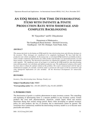
36
3. The demand rate is constant say D units per unit of time.
4. Shortages are permitted.
5. Delivery lead time is zero.
6. The holding cost, ordering cost remains constant over time.
4. MODEL FORMULATION
4.1 EOQ Model for Infinite Production Rate with Shortages
Figure (1) Inventory system with complete backlogging for Infinite production rate
Let Q be the number of items received or the inventory level at the beginning of the period.
From the figure (1), it is clear that inventory level decreases due to the constant demand say D
units per unit of time. Up to the time interval ),0( µ , there is no deterioration of the product but
after time µ=t , the product continuously deteriorates so the penalty cost can be incurred upon
for the time interval )t,( 1µ . The total variable cost per cycle time consists of the inventory
holding cost, set up cost and penalty cost. Since the demand rate is D units per unit time, the
total demand in one cycle of time-interval T is = DT
The number of items received at the commencement of the period is Q = DT (1)
For the time interval ),0( µ , no perishability occurs only demand is delivered during this period at
the rate of D units per unit time. But for the time interval )t,( 1µ , deterioration of the product
starts and time interval ),( 1 Tt shortage will occur. As a result, penalty cost has been imposed.
Case I: linear penalty cost function with Shortage
A linear penalty cost function µµπ ≥−= tttP ),()( , which gives the cost of keeping one unit
of product in stock until age t, where µ be the time period at which deterioration of product start
and π is constant.

37
Deterioration Cost
The cost due to the deterioration of the product delivered during the period dttt +, is given by
dtDt )( µπ − . Thus penalty cost due to the deterioration of the products delivered during the
time interval ),( 1`tµ is given by
Setup Cost
The setup cost of inventory for the period ),0( T given by
Holding Cost
Now the cost of holding inventory for the period ),0( T is given by
Shortage Cost
Now the cost of shortage for the period ),( 1 Tt is given by
∴The average total variable cost per unit time )(TC is given by
SHCHCSCDCTC +++=)( (From (2) to (5))

38
Differentiate equation (6) with respect to QandT
Then we get, the optimum cycle time *
T and expressed as
Then we get, the optimum order quantity *
Q by putting the value of *
T in equation (1)
Case II: Exponential penalty cost function with Shortage
An exponential penalty cost function ( ) µα µβ
≥−= −
tetP t
,1)( )(
which also gives the cost of
keeping one unit of product in stock until aget , where µ be the time period in which
deterioration of product start andα , β are constants. The cost due to the deterioration of the
product delivered during the period dttt +, is given by ( ) dtDe t
1)(
−−µβ
α
Deterioration Cost
The penalty cost due to the deterioration of the product delivered during the time interval ),( 1tµ
is given by

39
By using second order approximation of the exponential term )( 1 µβ −t
e in )(TC we get








−−−
−
+−+= )(1
2
)(
)(1 1
2
1
2
1 µβ
µβ
µβ
β
α
t
t
t
D
DC








−+= µβ
βµβ
α 1
22
1
22
t
t
D
Setup Cost
The set cost of inventory for the period ),0( T is given by
T
A
SC = (10)
Holding Cost
Now the cost of holding inventory for the period ),0( T is given by
DTQe
HQT
HC == wher,
2
2
2
HDT
= (11)
Shortage Cost
Now the cost of shortage for the period )( ,1 Tt is given by
∫−=
T
t
dtDcSHC
1
∫−=
T
t
dtcD
1
( )1tTcDSHC −−= (12)
SHCHCSCDCTC +++=)( (From (9) to (12))
T
cDt
cD
HDT
T
A
T
tD
T
D
T
tD 11
22
1
222
+−++−+=
αµββαµαβ
(13)

40
0
)(
=
∂
∂
T
TC
Then we get, the optimal cycle time *
T and expressed as
HD
tDcDttDDA
T
µαβαβµαβ 11
2
1
2
* 222 −+++
= (14)
Then we get, the optimal order quantity *
T in equation (1)
( )
H
tDcDttDDAD
Q
µαβαβµαβ 11
2
1
2
* 222 −+++
=
(15)
From the expression (14) and (15), it is clear that if 0=µ and παβ = then these two
expressions are same as (7) and (8).
4.2 EOQ Model for finite Production Rate with Shortages
In this model the assumption of infinite production rate is relaxed. The rate of production P units
per period is finite. The behavior of an inventory system in one cycle may be depicted as in figure
(2).
Figure (2) Inventory system with complete backlogging for finite production rate
From the Fig. (2), it is clear that initially the stock is zero and the production starts with a finite
rate )( DP > units per unit time while the demand is D units per unit time. Thus, the inventory
increases with a rate )( DP − units per unit time. Let the production continue for a period.
∴Inventory level at the end of the time Ω is Ω−= )( DPq

41
Let DP > be the number of items produced per unit time. If ""Q be the number of items
produced per production run then production will continue for a time
P
Q
=Ω
The time of one complete cycle
T
Q
T =
After time Ω , production is completed. Then the inventory level at the moment when the
production is completed is
P
Q
DPq )( −=






−=
P
D
Qq 1 ` (16)
Let us assume that the products do not deteriorate at the beginning of the production cycle. But
deteriorate after sometime of the production period. Let the perishability occurs after time µ=t
from the beginning of the cycle. The total variable cost per cycle time consists of the set up cost,
inventory holding cost and perishability cost.
Case I Linear penalty cost function with Shortage
A linear penalty cost function µµπ ≥−= tttP ),()( , which gives the cost of keeping one unit
of product in stock until age t, where µ be the time period at which deterioration of product start
and π is constant.
Holding Cost
The holding cost per cycle is given by
2
HqT
HC =






−=
P
DDHT
1
2
2
(17)
Deterioration Cost
The total number of units delivered in time )( µ−t is )( µ−tD and their production time is
P
tD )( µ−
where 1tt ≤<µ .
Therefore, the age of the product delivered at time ''t is given





 −
−−=
p
tD
t
)(
)(
µ
µ

42






−−=
P
D
t 1`)( µ
Since the total number of units to be delivered during a period ),( dttt + is Ddt . If linear
penalty cost function is used, then the cost due to deterioration of products delivered during the
period ),( dttt + is given by
( ) dt
P
D
tDDC
t
∫ 





−−=
1
1
µ
µπ








−+





−= 1
22
1
`22
1 t
t
P
D
D µ
µ
π








−+





−= 1
22
1
`22
1 t
t
P
D
D µ
µ
π (18)
Setup Cost
The setup cost of inventory for the period ),0( T is given by
T
A
SC = (19)
Shortage Cost
Now the cost of shortage for the period ),( 1 Tt is given by








−= ∫
T
t
dtDcSHC
1








−= ∫
T
t
dtcD
1
[ ]1tTcD −−= (20)
SHCHHCSCDCTC +++=)( (Form (17) to (20))
T
cDt
cD
P
DHDT
T
A
P
D
T
tD
P
D
T
D
P
D
T
Dt
1
1
22
1
1
2
11
2
1
2
+−






−++





−−





−+





−=
µπµππ
(21)

43
0
)(
=
∂
∂
T
TC
T and expressed as






−






−−





−++





−+
=
P
D
DH
t
P
D
D
P
D
tDcDt
P
D
DA
T
1
121212 1
2
11
2
*
µππµπ
(22)
Then we get, optimum order quantity *
T in equation (1)
H
P
D
t
P
D
D
P
D
tDcDt
P
D
DAD
Q






−












−−





−++





−+
=
1
121212 1
2
11
2
*
µππµπ
(23)
If ∞=P (i.e. production rate is infinite), then (22) and (23) coincide with (7) and (8).
Case II Exponential penalty cost function with Shortage
An exponential penalty cost function ( ) µα µβ
≥−= −
tetP t
,1)( )(
which also gives the cost of
keeping one unit of product in stock until aget , where µ be the time period at which
deterioration of product start and α and β are constants. The cost due to the deterioration of the
product delivered during the period dttt +, is given by ( ) dtDe t
1)(
−−µβ
α . Also if an
exponential penalty cost function is used by using second order approximation of the exponential
term exp 











−−
P
D
T 1)( µβ by taking παβ = the same equation (14) and (15) are obtained.
T and expressed as






−






−−





−++





−+
=
P
D
DH
t
P
D
D
P
D
tDcDt
P
D
DA
T
1
121212 1
2
11
2
*
µαβαβµαβ
(24)
Then we get, the optimum order quantity *
Q and it is expressed as

44






−












−−





−++





−+
=
P
D
H
t
P
D
D
P
D
tDcDt
P
D
DAD
Q
1
121212 1
2
11
2
*
µαβαβµαβ
(25)
5. NUMERICAL ILLUSTRATION
To illustrate the theoretical development, the following examples have been considered
P=40 units per day, D=20 units per day, H=Rs. 0.03 per day A=Rs. 50 per day, µ=1 days, α=5,
β=0.95, t1=0.03, c=1, π=3.14-
EOQ model for infinite production rate with shortage
Case I when linear penalty cost function is considered
Optimum cycle time days16*
=T .
Optimum order quantity units327*
=Q .
Case II when exponential penalty cost function is considered
=T .
=Q .
EOQ model for finite production rate with shortage
Case I when linear penalty cost function is considered
=T .
=Q .
Case II when exponential penalty cost function is considered
=T .
=Q .
6. SENSITIVITY ANALYSIS
The sensitivity analysis is carried out for checking the helpfulness of the EOQ model for infinite
and finite production rate with shortage with deference to the parameter
DPAHtc ,,,,,,,, 1βαµ on optimum cycle time *
T and optimum order quantity *
Q for both
proposed models. Results are shown in the table (1)

45
Table (1) optimum order quantity and optimum cycle time for infinite and finite production rate with
shortage

46
7. MANAGERIAL IMPLICATIONS
To study the effects of the parameters on the optimal results of the proposed models, a sensitivity
analysis is performed by transmuting the values of the key parameters piecemeal, keeping the
remaining parameters at their pristine levels. From the sensitivity analysis of example the
following managerial implications are found.
Infinite production rate with shortage
Linear penalty cost function
µ - Increase for the optimum cycle time as well as optimum order quantity.
α - Equal value for the optimum cycle time as well as optimum order quantity.
β - Equal value for the optimum cycle time as well as optimum order quantity.
c - Equal value for the optimum cycle time and increase the value for optimum order
quantity.
1t - Equal value for the optimum cycle time and decrease the value for optimum order
quantity.
H - Decrease for the optimum cycle time as well as optimum order quantity.
A - Increase for the optimum cycle time as well as optimum order quantity.
P - Equal value for the optimum cycle time as well as optimum order quantity.
D - Decrease the optimum cycle time as well as increase the optimum order quantity.
Exponential penalty cost function
α - Increase for the optimum cycle time as well as optimum order quantity.
β - Increase for the optimum cycle time as well as optimum order quantity.
quantity.
quantity.
P - Equal value for the optimum cycle time as well as optimum order quantity.
D - Decrease the optimum cycle time as well as increase the optimum order quantity.

47
Finite production rate with shortage
Linear penalty cost function
α - Equal value for the optimum cycle time as well as optimum order quantity.
quantity.
quantity.
P - Decrease the optimum cycle time as well as increase the optimum order quantity.
D - Increase the optimum cycle time as well as Decrease the optimum order quantity.
Exponential penalty cost function
α - Increase for the optimum cycle time as well as optimum order quantity.
c - Equal value for the optimum cycle time as well as optimum order quantity.
quantity.
P - Decrease the optimum cycle time as well as increase the optimum order quantity.
D - Increase the optimum cycle time as well as Decrease the optimum order quantity.
8. CONCLUSION
The purpose of this study is to present an EOQ model for time deteriorating items i.e. for those
perishable products which do not deteriorate for some period of time and after that time they
continuously deteriorate with time for both infinite and finite production rate with shortage. The
proposed model, the shortages are considered to be completely backlogging. In this model we
can use the linear penalty cost and exponential penalty cost function. In production rate is
postulated to be finite and infinite.
In this manuscript, the idea of the continuous deterioration of utility for an individual perishable
product, and a measure for the utility deterioration as a linear and an exponential penalty cost
function with shortages and completely backlogging are introduced into the EOQ model.

48
Computer Matlab coding is additionally developed to receive the best result and present
numerical examples to illustrate the model. Analytical solutions of the model are illustrated with
the help of suitable numerical examples. The model is solved analytically by determining the
optimum cycle time as well as optimum order quantity. To conclude, sensitivity of the optimal
solution with respect to changes in different parameter values is carried out and some managerial
implications are obtained of the proposed model.
ACKNOWLEDGEMENT
The authors greatly appreciate the reviewers for their valuable and insightful comments, which
helped in improving the paper. The author also wishes to thank the Journal Publishing Editor for
their helpful suggestions, which have led to a significant improvement in the earlier version of
the paper. The first author research work is supported by DST INSPIRE Fellowship, Ministry of
Science and Technology, Government of India under the grant no. DST/INSPIRE
Fellowship/2011/413A dated 15.01.2014 and UGC – SAP, Department of Mathematics,
Gandhigram Rural Institute – Deemed University, Gandhigram – 624302, Tamilnadu, India.
REFERENCES
[1] Bahari-Kashani,H. (1989) “ Replenishment schedule for deteriorating items with time proportional demand”.
Journal of the operational Research Society, Vol. 40, No. 1, pp. 75- 81.
[2] Burwell T. H., Dave D. S., Fitzpatrick K. E & Roy M. R. (1997).”Economic lot size model for price-dependent
demand under quantity and freight discounts”. International Journal of Production Economics, Vol. 48, No.2, pp.
141-155.
[3] Chung, K. J & Ting, P. S. (1993) “A heuristic for replenishment of deteriorating items with a linear trend in
demand”, Journal of the Operational Research Society, Vol. 44, No.12, pp.1235-1241.
[4] Covert, R. P & Philip, G. C. (1973). “An EOQ model for items with Weibull distributed deterioration”. AIIE
Transactions, Vol. 5, No.4, pp. 323-326.
[5] Deb, M & Chaudhari, K. A. (1987). “Note on the heuristic for replenishment of trended inventories considering
shortages”. Journal of the Operational Research Society, Vol. 38, No. 5, pp. 459-463.
[6] Dye, C. Y & Hsieh, T. P. (2012). “An optimal replenishment policy for deteriorating items with effective
investment in preservation technology”, European Journal of Operational Research, Vol. 218, No.1, pp. 106-112.
[7] Fauza, G., Amer, Y & Lee, S. H. (2013). “A map of research in inventory models for perishable items from the
perspective of supply chain management”. IEEE Symposium on Business, Engineering and Industrial
Applications Malaysia:IEEE.
[8] Ferguson, M., Jayaraman, V & Souza, G. C. (2007). Note: An application of the EOQ model with nonlinear
holding cost to inventory management of perishable. European Journal of Operational Research, Vol. 180, No.1,
pp.485-490.
[9] Fujiwara, O & Perera, U. L. J. S. R. (1993). “EOQ model for continuously deteriorating products using linear
and exponential penalty costs”. European Journal of Operational Research, Vol. 70, No.1, pp.104-114.
[10] Ghare, P & Schrader, G. (1963). “A model for exponentially decaying inventory”. Journal of Industrial
Engineering, Vol.14, No. 5, pp.238-243.
[11] Ghosh, S. K & Chaudhuri, K. S. (2006). “An EOQ model with a quadratic demand, time - proportional
deterioration and shortages in all cycles”. International Journal of Systems Sciences, Vol.37, No.10, pp. 663 -
672.
[12] Giri, B. C. Chakrabarti, T & Chaudhuri, K. S. (2000). “A note on a lot sizing heuristic for deteriorating items
with time varying demands and shortages”. Computers and Operations Research, Vol. 27, No. 6, pp. 495-505.
[13] Giri, B. C., Chakrabarti, T & Chaudhuri, K. S. (1997). “Heuristic models for deteriorating items with shortages
and time-varying demand and costs”. International Journal of Science, Vol. 28, No.2 pp. 153-159.
[14] Goswami, A & Chaudhuri, K. S. (1991). “An EOQ model for deteriorating items with storages and a linear trend
in demand”. Journal of the Operational Research Society, Vol. 42, No. 12, pp. 1105-1110.
[15] Goyal, S. K. (1988). “A heuristic for replenishment of trended inventories considering shortages”. Journal of the
Operational Research Society, Vol. 39, No. 9, pp. 885-887.
[16] Hariga, M. (1994). “The inventory lot-sizing problem with continuous time varying demand and shortages”.
Journal of the Operational Research Society, Vol. 45, No.7, pp. 827-837.

49
[17] Hariga, M. A & Bankherouf, L. (1994). “Optimal and heuristic inventory replenishment models for deteriorating
items with exponential time-varying demand”. European Journal of Operational Research, Vol.79, No.1, pp.
123-137.
[18] Jain, K & Silver, E. A. (1994). “Lot sizing for a product subject to obsolescence or perishability”. European
Journal of Operational Research, Vol. 75, No.2, pp. 287-295.
[19] Jalan, A. K & Chaudhari, K. S. (1999). “Structural properties of an inventory system with deterioration and
trended demand”. International Journal of Systems Science, Vol. 30, No. 6, 627-633.
[20] Jalan, A. K & Chaudhuri, K. S. (1999). “An EOQ model for deteriorating items in a declining market with SFI
policy”. Korean Journal of Computational and Applied Mathematics, Vol. l6, No. 2, pp. 437 - 449.
[21] Khanra, S & Chaudhuri, K. S. (2003). “A note on an order level inventory model for a deteriorating item with
time dependent quadratic demand”. Computer and Operations Research, Vol.30, No.12, pp. 1901 - 1916.
[22] Lin, C, Tan, B & Lee, W. C. (2000). “An EOQ model for deteriorating items with time-varying demand and
shortages”. International Journal of Systems Science, Vol. 31, No. 3, pp. 391–400.
[23] Liu, L & Lian, Z. (1999). “(s, S) continuous review models for inventory with fixed life- times”. Operations
Research, Vol. 47, No. 1, pp. 150-158.
[24] Maihami, R & Abadi, I. N. K. (2012). “Joint control of inventory and its pricing for non-instantaneously
deteriorating items under permissible delay in payments and partial backlogging”. Mathematical and Computer
Modelling, Vol.55, No.5, pp.1722 - 1733.
[25] Mary Latha, K. F & Uthayakumar, R. (2014). “An inventory model for increasing demand with probabilistic
deterioration, permissible delay and partial backlogging”. International Journal of Information and Management
Sciences, Vol. 25, No. 4, pp.297-316.
[26] Misra, R. B. (1975).“Optimum production lot size model for a system with deteriorating inventory”.
International Journal of Production Research, Vol. 13, No. 5, pp. 495-505.
[27] Mitra, A., Cox, J. F & Jesse, R. R. (1984). “A note on deteriorating order quantities with a linear trend in
demand”. Journal of Operational Research Society, Vol.35, pp. 141 - 144.
[28] Mondal, B., Bhunia, A. K. & Maiti, M. (2003). “An inventory system of ameliorating items for price dependent
demand rate”. Computers and Industrial Engineering, Vol. 45, No.3, pp. 443-456.
[29] Nandakumar, P & Morton, T. E. (1990). “Near myopic heuristic for the fixed life perishability problem”.
Management Science, Vol. 18, pp.1490-1498.
[30] Palanivel, M & Uthayakumar, R. (2014). “A production-inventory model with variable production cost and
probabilistic deterioration”. Asia Pacific Journal of Mathematics, Vol.1, No. 2, pp.197-212.
[31] Perry, D. A. (1997). “Double band control policy of a Brownian perishable inventory system, Probability”.
Engineering and Informational Sciences, Vol. 11, No.3, pp. 361-373.
[32] Ranjana, G & Meenakshi, S. (2009). “EOQ Model for Time-Deteriorating Items Using Penalty cost”. Journal of
Reliability and Statistical Studies, Vol. 2, No.2, pp. 67-76.
[33] Shah, N. H, Soni, H. N & Patel, K. A. (2013). “Optimizing inventory and marketing policy for non-instantaneous
deteriorating items with generalized type deterioration and holding cost rates”.Omega, Vol.41, No.2, pp. 421
430.
[34] Sicilia, J., Gonzalez De -la-Rosa, M., Febles-Acosta, J & Alcaide-Lopezde- Pablo, D. (2014). “An inventory
model for deteriorating items with shortages and time-varying demand”. International Journal of Production
Economics, Vol.155, pp. 155 - 162.
[35] Teng, J. T & Chang, C. T. (2005). “Economic production quantity models for deteriorating items with price and
stock dependent demand”. Computers and Operations Research, Vol. 32, No.2, pp. 297-308.
[36] Tripaty, C. K & Mishra, U. (2010). “An Inventory Model for Weibull Time –Dependence Demand Rate with
Completely Backlogged Shortages”. International Mathematical Forum, Vol. 5, No. 54, pp. 2675-2687.
[37] Vijayashree, M & Uthayakumar, R. (2014). “A two stage supply chain model with selling price Dependent
demand and investment for quality Improvement”. Asia Pacific Journal of Mathematics, Vol. 1, No. 2, pp. 182-
196.
[38] Wee, H.M. (1995). “A deterministic lot-size inventory model for deteriorating items with shortages and a
declining market”.Computers and Operations Research, Vol. 22, No. 3, pp. 345 - 356.
[39] Weiss, H. J. (1982). “Economic order quantity models with nonlinear holding cost”. European Journal of
Operational Research, Vol.9, pp.56-60.
[40] You, S. P. (2005). “Inventory policy for products with price and time-dependent demands”. Journal of the
Operational Research Society, Vol. 56, No. 7, pp. 870-873.

50
AUTHORS
M. Vijayashree is a full time research scholar in the Department of Mathematics
at The Gandhigram Rural Institute – Deemed University, Gandhigram, India. She
received her B.Sc in Mathematics from M.V.M Govt Women’s Arts College,
Dindigul, Tamilnadu, India in 2007 and M.Sc. Tech (IMCA) in Industrial
Mathematics with Computer Applications from The Gandhigram Rural Institute-
Deemed University, Gandhigrm, Dindigul, Tamilnadu, India in 2010. Currently,
she is a Senior Research Fellow under DST INSPIRE, New Delhi; in the
Department of Mathematics, The Gandhigram Rural Institute – Deemed
University, Gandhigram, India. Her research interests include the following fields: operations research,
inventory management and control, supply chain management.
R. Uthayakumar is currently an Professor in the Department of Mathematics at
The Gandhigram Rural Institute – Deemed University, Gandhigram, India. He
received his M.Sc in Mathematics from American College, Madurai, India in 1989
and PhD in Mathematics from The Gandhigram Rural Institute – Deemed
University, Gandhigram, India in 2000. He has published about 121 papers in
international and national journals. His research interests include the following
fields: operations research, industrial engineering and fractal analysis fuzzy spaces
and inventory models.

AN EOQ MODEL FOR TIME DETERIORATING ITEMS WITH INFINITE & FINITE PRODUCTION RATE WITH SHORTAGE AND COMPLETE BACKLOGGING

Recommended

Recommended

More Related Content

Similar to AN EOQ MODEL FOR TIME DETERIORATING ITEMS WITH INFINITE & FINITE PRODUCTION RATE WITH SHORTAGE AND COMPLETE BACKLOGGING

Similar to AN EOQ MODEL FOR TIME DETERIORATING ITEMS WITH INFINITE & FINITE PRODUCTION RATE WITH SHORTAGE AND COMPLETE BACKLOGGING (20)

Recently uploaded

Recently uploaded (20)

AN EOQ MODEL FOR TIME DETERIORATING ITEMS WITH INFINITE & FINITE PRODUCTION RATE WITH SHORTAGE AND COMPLETE BACKLOGGING