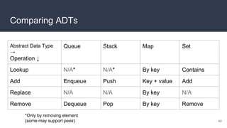
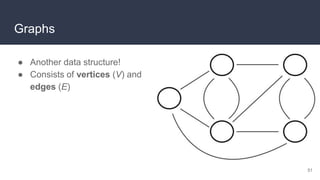
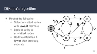
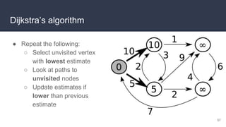
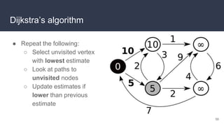
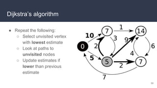
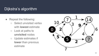
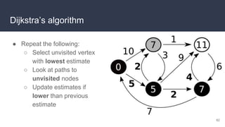
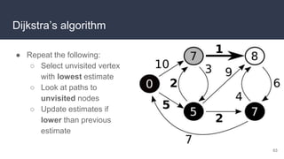
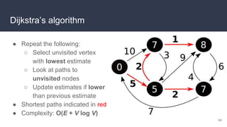
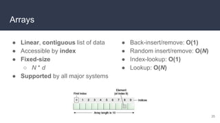
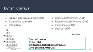
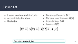
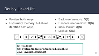
This document provides an overview of algorithms and data structures. It covers sorting algorithms like insertion sort, bubble sort, merge sort, and quicksort. It discusses complexity analysis using Big O notation and compares the time complexities of different sorting and searching algorithms. Common linear and nonlinear data structures are explained like arrays, linked lists, stacks, queues, trees, and hash tables. Abstract data types like maps, sets, queues and stacks are also introduced. Dijkstra's algorithm for finding shortest paths in graphs is described.

1. Algorithms & Data Structures
Lecture 1
L.J. Bel
iCSC 2018

2. Outline
Lecture I
1. Motivation
2. Sorting algorithms
3. Complexity analysis
4. Linear data structures
Lecture II
5. Nonlinear data structures
6. Abstract data types
7. Dijkstra’s algorithm
8. Summary
2

3. Attention!
Lecture aimed at non-computer scientists.
Focus is on explaining concepts,
rather than technical correctness.
3

4. 1. Motivation
4

5. Motivation
● Algorithms
● Data Structures
1. Everything running on your
computer is an algorithm
2. Analysing them is paramount
to writing, maintaining and
improving them
3. Several tools exist to help
achieve this
5

6. Motivation
● Algorithms
● Data Structures
1. Data Structures define how
data is stored in RAM
2. Many variations, each with
advantages and
disadvantages
3. Strongly coupled to algorithmic
complexity
6

7. 2. Sorting algorithms
7

8. Sorting
● Suppose we have some unsorted list
● We want to make it sorted
8
3 1
5
6 8 7 2 4
3 4
2
1 5 6 7 8

9. N steps
N steps
● In pseudocode:
i ← 1
while i < length(A)
j ← i
while j > 0 and A[j-1] > A[j]
swap A[j] and A[j-1]
j ← j - 1
end while
i ← i + 1
end while
Insertion sort
● “Naive” sorting algorithm
● One-by-one, take each
element and move it
● When all elements have been
moved, list is sorted!
9
● In pseudocode:
i ← 1
while i < length(A)
j ← i
while j > 0 and A[j-1] > A[j]
swap A[j] and A[j-1]
j ← j - 1
end while
i ← i + 1
end while
Total: N² steps
By Swfung8 (Own work) [CC BY-SA
3.0], via Wikimedia Commons

10. Bubble sort
● Traverse the list, taking pairs
of elements
● Swap if order incorrect
● Repeat N times
● Now it’s sorted!
10
Total: N² steps
By Swfung8 (Own work) [CC BY-SA 3.0],
via Wikimedia Commons
N steps
N steps

11. Intermezzo: Divide and conquer
● Generic algorithm strategy
○ Divide the problem into smaller parts
○ Solve (conquer) the problem for each part
○ Recombine the parts
● Straightforward to parallelise
● Closely related to map-reduce
● Has been advocated by Caesar, Machiavelli, Napoleon...
11

12. Merge sort
● Much smarter sort
○ Split the dataset into chunks
○ Sort each chunk
○ Merge the chunks back together
● Example of divide-and-conquer
● Splitting & sorting takes log₂(N) steps
● Merging takes N steps
12
By Swfung8 (Own work) [CC BY-SA 3.0],
via Wikimedia Commons
Total: N log(N) steps

13. 3. Complexity analysis
13

14. Complexity – O
● We use “Big-O” notation
● Represents an upper bound
● Ignores constants
● Only shows dominant term
● In these examples: N is
amount of data
● Linear: O(N)
○ O(N) = O(2*N) = O(k*N + m)
for any constants k, m
● Quadratic: O(N²)
○ O(N²) = O(a*N² + b*N + c)
for any constants a, b, c
14

15. Complexity – O
● Roughly three categories, in decreasing
order:
○ Exponential – O(kN)
○ Polynomial – O(Nk)
○ Polylogarithmic – O(log(N)k)
● This is an abstraction!
○ Does not directly relate to runtimes
○ A good O(N²) algorithm may be faster than
a bad O(log(N)) one
○ Depends on your input data! 15
By Cmglee (Own work) [CC BY-SA 4.0],
via Wikimedia Commons

16. Complexity – O
● Remember: it’s an upper
bound!
● And it’s a property (not an
equivalence relation)!
○ O(N) = O(N²)
○ But O(N²) ≠ O(N)
● O(N) = O(2N)
● 2N = O(N)
● N² + N = O(N²)
● O(N²) + O(N) = O(N²)
● O(log(N)) + O(N) = O(N)
● O(1) → used for constant time
16

17. Complexity – O
● Formal definition:
f(N) = O(g(N)) ↔
∃ N₀, M : ∀ N > N₀ : f(N) ≤ M g(N)
● In words: starting from N₀, f is bounded
from above by g (up to some constant M)
17
By Cmglee (Own work) [CC BY-SA 4.0],
via Wikimedia Commons

18. Complexity – Ω
● Ω: lower bound
○ Formal definition:
f(N) = Ω(g(N)) ↔
∃ N₀, M : ∀ N > N₀ : f(N) ≥ M g(N)
○ In words: starting from N₀, f is bounded
from below by g (up to some constant M)
● Examples:
○ N = Ω(log(N))
○ N² = Ω(N)
18
By Cmglee (Own work) [CC BY-SA 4.0],
via Wikimedia Commons

19. Complexity – Θ
● Θ: exact bound
○ Formal definition:
f(N) = Θ(g(N)) ↔
f(N) = O(g(N)) and f(N) = Ω(g(N))
● Examples:
○ N = Θ(N)
○ 2N = Θ(N)
○ 3N²+5N+1 = Θ(N²)
○ N ≠ Θ(N²) (even though N = O(N²))
19
By Cmglee (Own work) [CC BY-SA 4.0],
via Wikimedia Commons

20. One more sorting example: Quicksort
● Pick an element, called pivot
● Partitioning: reorder the
array so that the pivot is in
the correct place
● Recursively apply the above
steps to the sub-arrays on
either side of the pivot
20
● Randomised-quicksort:
select the pivot randomly

21. Stable sorting
● A sorting algorithm is stable
iff it conserves the order of
equal elements
21

22. Comparison of algorithms
22
Algorithm Stable? Complexity
Insertion sort ✅ O(N²)
Bubble sort ✅ O(N²)
Merge sort ✅ O(N log(N))
Quicksort ❌ ?

23. 4. Linear data structures
23

24. Memory
24

25. Arrays
● Linear, contiguous list of data
● Accessible by index
● Fixed-size
○ N * d
● Supported by all major systems
25
● Back-insert/remove: O(1)
● Random insert/remove: O(N)
● Index-lookup: O(1)
● Lookup: O(N)

26. Dynamic arrays
● Linear, contiguous list of data
● Accessible by index
● Resizable
26
C++: std::vector
Python: list
C#: System.Collections.ArrayList
Java: java.util.ArrayList
● Back-insert/remove: O(1)*
● Random insert/remove: O(N)
● Index-lookup: O(1)
● Lookup: O(N)
*Amortised.

27. Pointers
27
By Sven (Own work) [CC BY-SA
3.0],
via Wikimedia Commons

28. Linked list
● Linear, contiguous list of data
● Accessible by iteration
● Resizable
28
● Back-insert/remove: O(1)
● Random insert/remove: O(N)
● Index-lookup: O(N)
● Lookup: O(N)
C++: std::forward_list

29. Doubly Linked list
● Pointers both ways
● Uses more memory, but allows
iteration both ways
29
● Back-insert/remove: O(1)
● Random insert/remove: O(N)
● Index-lookup: O(N)
● Lookup: O(N)
C++: std::list
C#: System.Collections.Generic.LinkedList
Java: java.util.LinkedList

30. Binary search
● Searches a sorted linear data structure
● Takes Θ(log(N))
● Example of divide and conquer
30
By AlwaysAngry (Own work) [CC BY-SA 4.0],
via Wikimedia Commons

31. Algorithms & Data Structures
Lecture 2
L.J. Bel
iCSC 2018

32. Outline
Lecture I
1. Motivation
2. Sorting algorithms
3. Complexity analysis
4. Linear data structures
Lecture II
5. Nonlinear data structures
6. Abstract data types
7. Dijkstra’s algorithm
8. Summary
32

33. 5. Nonlinear data structures
33

34. Recall: Binary search
● Searches a sorted linear data structure
● Takes Θ(log(N))
● … let’s use this as inspiration for a data structure!
34
By AlwaysAngry (Own work) [CC BY-SA 4.0],
via Wikimedia Commons

35. Binary search trees
● Tree structure
● Pointers between nodes
○ To the right: only larger
○ To the left: only smaller
● Allows easy sorted iteration
● Search/insert/delete:
all O(log(N))
35

36. Hash tables
● Idea: create buckets
numbered 1 to B
● For each item, compute in
which bucket it belongs
● Put the item in that bucket
● Search/insert/delete:
all O(1)
36
By Jorge Stolfi (Own work) [CC BY-SA 3.0],
via Wikimedia Commons

37. Hash tables
● Problem: clashing hashes!
● Solution: replace entry with
linked list (chaining)
● New problem: load factor
can become too high!
● Solution: copy to new table
with more buckets
37
By Jorge Stolfi (Own work) [CC BY-SA 3.0],
via Wikimedia Commons

38. Comparing data structures
38
Data structure →
Operation ↓
Dynamic
array
Linked list Binary
search tree
Hash table
Lookup O(N) O(N) O(log(N)) O(1)
Indexed lookup O(1) O(N) N/A N/A
Back-insert O(1)* O(1) O(log(N)) O(1)*
Random insert O(N) O(N) N/A N/A
Remove O(N) O(N) O(log(N)) O(1)*
*Amortised.

39. 6. Abstract data types
39

40. Why “Abstract”?
● Abstract Data Type (ADT) does not define a real data structure
○ Only defines an interface
○ Implemented using one of the “real” data structures
● Usually limits operations compared to actual DS
● Enhances flexibility
Related to several core programming principles:
● Program against the interface, not the implementation!
● Use high cohesion, loose coupling
● Separate the concerns 40

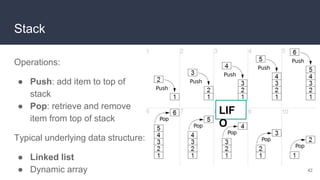
41. Operations:
● Enqueue: add item to beginning
of queue
● Dequeue: retrieve and remove
item from end of queue
Typical underlying data structure:
● Linked list
● Dynamic array
Queue
41
By Vegpuff (Own work) [CC BY-SA 3.0],
via Wikimedia Commons
FIF
O

42. Operations:
● Push: add item to top of
stack
● Pop: retrieve and remove
item from top of stack
Typical underlying data structure:
● Linked list
● Dynamic array
Stack
42
LIF
O

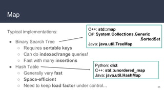
43. Map
● Map: dataset that maps
(associates) keys to values
● Keys are unique
(values need not be)
● Values can be retrieved by
key
● Not indexed…
○ ...although an array could
be seen as a map with
integer keys! 43
By Jorge Stolfi (Own work) [CC BY-SA 3.0],
via Wikimedia Commons

44. Map
Operations:
● Lookup: retrieve value for a
key
● Insert: add key-value pair
● Replace: replace value for a
specified key
● Remove: remove key-value
pair
44
By Jorge Stolfi (Own work) [CC BY-SA 3.0],
via Wikimedia Commons

45. Map
Typical implementations:
● Binary Search Tree
○ Requires sortable keys
○ Can do indexed/range queries!
○ Fast with many insertions
● Hash Table
○ Generally very fast
○ Space-efficient
○ Need to keep load factor under control... 45
Python: dict
C++: std::unordered_map
Java: java.util.HashMap
C++: std::map
C#: System.Collections.Generic
.SortedSet
Java: java.util.TreeMap

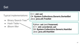
46. Set
● Set: dataset that contains
certain values
● No ordering, no
multiplicity
● A value is either present
or not
46
Adapted by L.J. Bel from Jorge Stolfi (Own work) [CC BY-SA 3.0],
via Wikimedia Commons

47. Set
Operations:
● Contains: check whether a
value is present
● Add: add a value
● Remove: remove a value
47
Adapted by L.J. Bel from Jorge Stolfi (Own work) [CC BY-SA 3.0],
via Wikimedia Commons

48. Set
Typical implementations:
● Binary Search Tree
● Hash Table
● Bloom filter
48
Python: set (and frozenset)
C++: std::unordered_set
C#: System.Collections.Generic.HashSet
Java: java.util.HashSet
C++: std::set
C#: System.Collections.Generic.SortedSet
Java: java.util.TreeSet

49. Comparing ADTs
49
Abstract Data Type
→
Operation ↓
Queue Stack Map Set
Lookup N/A* N/A* By key Contains
Add Enqueue Push Key + value Add
Replace N/A N/A By key N/A
Remove Dequeue Pop By key Remove
*Only by removing element
(some may support peek)

50. 7. Dijkstra’s algorithm
50

51. Graphs
● Another data structure!
● Consists of vertices (V) and
edges (E)
51

52. Graphs
● Another data structure!
● Consists of vertices (V) and
edges (E)
● Edges may carry a weight
52

53. Graphs
● Another data structure!
● Consists of vertices (V) and
edges (E)
● Edges may carry a weight
Directed graph:
● Edges are directed
53

54. Pathfinding
● Problem: find shortest path
from A to B
● Shortest is defined as lowest
total edge weights
54

55. Dijkstra’s algorithm
● Algorithm to obtain shortest
path from a given vertex to
any other vertex
● Example of greedy algorithm
● Initially: set shortest-path
estimates to 0 for start vertex
and ∞ for the others
55

56. Dijkstra’s algorithm
● Repeat the following:
○ Select unvisited vertex
with lowest estimate
○ Look at paths to
unvisited nodes
○ Update estimates if
lower than previous
estimate
56

57. Dijkstra’s algorithm
● Repeat the following:
○ Select unvisited vertex
with lowest estimate
○ Look at paths to
unvisited nodes
○ Update estimates if
lower than previous
estimate
57

58. Dijkstra’s algorithm
● Repeat the following:
○ Select unvisited vertex
with lowest estimate
○ Look at paths to
unvisited nodes
○ Update estimates if
lower than previous
estimate
58

59. Dijkstra’s algorithm
● Repeat the following:
○ Select unvisited vertex
with lowest estimate
○ Look at paths to
unvisited nodes
○ Update estimates if
lower than previous
estimate
59

60. Dijkstra’s algorithm
● Repeat the following:
○ Select unvisited vertex
with lowest estimate
○ Look at paths to
unvisited nodes
○ Update estimates if
lower than previous
estimate
60

61. Dijkstra’s algorithm
● Repeat the following:
○ Select unvisited vertex
with lowest estimate
○ Look at paths to
unvisited nodes
○ Update estimates if
lower than previous
estimate
61

62. Dijkstra’s algorithm
● Repeat the following:
○ Select unvisited vertex
with lowest estimate
○ Look at paths to
unvisited nodes
○ Update estimates if
lower than previous
estimate
62

63. Dijkstra’s algorithm
● Repeat the following:
○ Select unvisited vertex
with lowest estimate
○ Look at paths to
unvisited nodes
○ Update estimates if
lower than previous
estimate
63

64. Dijkstra’s algorithm
● Repeat the following:
○ Select unvisited vertex
with lowest estimate
○ Look at paths to
unvisited nodes
○ Update estimates if lower
than previous estimate
● Shortest paths indicated in red
● Complexity: O(E + V log V)
64

65. 8. Summary
65

66. Summary
● Concepts ● Divide and conquer
● Complexity
○ O, Θ, Ω
● (Un)stable sorting
● Pointers
66

67. Summary
● Concepts
● Sorting algorithms ● Insertion sort
● Bubble sort
● Merge sort
● Quicksort
67

68. Summary
● Concepts
● Sorting algorithms
● Data structures
● Arrays
● Dynamic arrays
● (Doubly) linked lists
● Binary search trees
● Hash tables
● (Directed) graphs
68

69. Summary
● Concepts
● Sorting algorithms
● Data structures
● Abstract data types
● Queues
● Stacks
● Maps
● Sets
69

70. Summary
● Concepts
● Sorting algorithms
● Data structures
● Abstract data types
● Algorithms
● Binary search
● Dijkstra’s algorithm
70